R E V I E W
Open Access
Cosinor-based rhythmometry
Germaine Cornelissen
Correspondence:
Halberg Chronobiology Center, University of Minnesota, 420 Delaware Street SE, 55455 Minneapolis, MN, USA
Abstract
A brief overview is provided of cosinor-based techniques for the analysis of time series in chronobiology. Conceived as a regression problem, the method is applicable to non-equidistant data, a major advantage. Another dividend is the feasibility of deriving confidence intervals for parameters of rhythmic components of known periods, readily drawn from the least squares procedure, stressing the importance of prior (external) information. Originally developed for the analysis of short and sparse data series, the extended cosinor has been further developed for the analysis of long time series, focusing both on rhythm detection and parameter estimation. Attention is given to the assumptions underlying the use of the cosinor and ways to determine whether they are satisfied. In particular, ways of dealing with non-stationary data are presented. Examples illustrate the use of the different cosinor-based methods, extending their application from the study of circadian rhythms to the mapping of broad time structures (chronomes).
Keywords:Chronobiology, Chronome, Circadian, Cosinor, External information, Regression, Rhythm parameters, Stationarity
Introduction
Non-random variations are found as a function of time at the cellular level, in tissue cul-ture, as well as in multi-cellular organisms at different levels of physiologic organization [1]. Multi-frequency rhythms usually account for a sizeable portion of the variability [2]. While there is presently much interest in studying circadian rhythms, the biological time structure covers many different ranges of periods beyond the 24-hour day, from fractions of seconds in single neurons to seconds in the cardiac and respiratory cycles, and a few hours in certain endocrine functions. Cycles with periods of about a week, about a month, and about a year are also ubiquitous, as are some other newly discovered cycles with periods of about 5 and 16 months, and much longer periods [3].
The partly built-in nature of circadian rhythms [4,5] is now widely accepted, as is the fact that they are amenable to synchronization by cycles in the environment (e.g., light-ing and feedlight-ing schedules) [6]. More generally, environmental geophysical cycles such as the day-light cycle, the tides, the phases of the moon, the seasons, as well as a host of other cycles shared between living organisms and the environment in which they evolved, all serve as synchronizers for partly endogenous rhythms [7,8].
The application of chronobiology and its concepts to biology and medicine depends upon the quantitative evaluation of data collected as a function of time. The inclusion of time as a primordial factor in chronobiological investigations broadens the scope of methods for data analysis. The methods presented herein serve the purposes of rhythm
the system (instrument, sensor) to measure a biological variable, yielding a set of data at discrete sampling times (ti, i = 1, 2,…, N). Whether the variable examined is discrete (e.g., mitotic counts) or continuous (e.g., oral temperature), the numerical values attrib-uted to Yiare limited in accuracy and precision by the instrumentation used. Any finite variation of a biological system takes place during a non-zero time interval rather than instantaneously. In terms of data analysis, this means that there is a cut-off frequency fS beyond which the spectrum of the biological variations is practically zero [10]. Whether the transducer used to measure a given biological variable is analog or digital, it takes a certain time for it to respond and deliver a reading, so that rhythms with periods shorter than this response time cannot be assessed, and rhythms with a period close to it will be distorted [10]. In other words, a cut-off frequency fTcan be defined as the minimal frequency such that for f > fT the output signal remains practically constant (no variation in the data can be assessed). This means that too dense measurements are redundant and do not bring additional information. In the case of equidistant data
obtained at Δt intervals, it has been recommended to choose Δt≤1/4fT to assure a
good approximation of Y(t) [11].
For chronobiological applications, this sampling requirement (to be able to recon-struct changes as a function of time in the context of the theory of signal processing) is often difficult to meet. Instead, sampling is used in its statistical meaning, where it refers to the selection of a few items from a population to draw inferences for that population. In terms of a data series, the selection of a sampling interval Δt > 1/fT al-lows only some features of the biological variations to be assessed. In the absence of ex-ternal information, for data collected over an observation span T, only oscillations with periods in the range of T up to 2Δt can be assessed. The resolution with which a
sig-nal’s period can be determined also depends on T: in frequency terms, the smallest
difference in frequency between two distinct signals is 1/T. The highest (no longer as-sessable) frequency, 1/2Δt, is called the Nyquist frequency, fN. Within the field of infor-mation theory, this is known as the Nyquist-Shannon theorem, which states that if a function Y(t) contains no frequencies higher than fN, it is completely determined by sampling Y(t) at intervals of 1/2fN.
estimate of uncertainty (experimental error or noise) used to derive statistical signifi-cance (P-values) and confidence intervals. Noise originates from variations in the bio-logical system considered not to be part of the deterministic portion of the signal, from errors external to the system (errors of experimentation, of observation, and/or of measurement), and from the transducer and sampler (instrumentation error). Reducing the experimental error increases the precision of experiments. Randomization is an important aspect of study design that allows researchers to proceed as though the as-sumption of independence of the observation errors is true, which is critical in applying a test of significance. Although randomization cannot guarantee independence, it re-duces the correlation that tend to characterize errors associated with experimental material (experimental unit or data) adjacent in space or time, while also improving ac-curacy. Control relates to the amount of balancing, blocking and grouping of the ex-perimental units [12].
The number of replications needed for a given probability of detecting a given differ-ence with statistical significance depends on the standard error per experimental unit [13]. This means that small sample sizes can easily detect large differences, whereas small differences require larger sample sizes. When dealing with rhythmic variables, a sizeable portion of the variance stems from the rhythmic variation. Assessing the rhythmic behavior is thus important to reduce the error term. One important feature of chronobiological study designs is that rhythm stage is often the primary factor, as when assessing the relative efficacy or toxicity of a given treatment administered at dif-ferent stages of the circadian rhythm. The power of testing for a time effect is usually only slightly affected by the number of timepoints considered when results are ana-lyzed by cosinor, but not when performing an analysis of variance. This difference in approach accounts in part for the controversy between classical designs advocating fewer test groups [14] and chronobiological designs recommending at least 6 time-points per cycle [15-17].
In the framework of chronobiological study designs, three kinds of data can be distin-guished, which determine the choice of method for their analysis and how the results can be interpreted. Longitudinal sampling corresponds to obtaining data on the same individual (experimental unit) as a function of time. One example is the around-the-clock monitoring of blood pressure at about 30-minute intervals for 7 days. Results apply to this particular individual. Transverse (cross-sectional) sampling consists of obtaining only one value per individual (experimental unit), different individuals pro-viding data at the same or different sampling times. Time series of survival times are one example of transverse data. When individuals represent a random sample of a given population, results can be generalized for that population. Hybrid (linked cross-sectional) sampling consists of taking a few serial measurements from several individ-uals (experimental units). For instance, circulating prolactin is determined at 20-minute intervals for 24 hours in women at low or high familial risk of developing breast cancer later in life. The circadian rhythm can be determined for each woman and summarized across all women in each group for assessing any difference as a function of breast can-cer risk [18]. When individuals represent a random sample of their respective popula-tions, results can be generalized to these populations.
pressure has been used to guide the timing of administration of anti-hypertensive
medication while also providing information regarding the patient’s response to
treatment [22].
Summary statistics
Before proceeding with any data analysis, it is recommended to first plot the data as a function of time. Such a chronogram can be informative in several ways. The presence of obvious rhythmicity may be recognized and its relative prominence as compared to the noise may be qualitatively (macroscopically) assessed. When sam-pling covers several cycles, some measure of the cycle-to-cycle variability can be gained. The presence of any increasing or decreasing trends can be observed, as is the existence of any outliers. After curve fitting, a chronogram of residuals can also provide valuable information regarding the adequacy of the model, and the need for data transformation.
A histogram should also be prepared to obtain an estimate of the mean value with its standard deviation, and to check on the assumption of normality. For instance, a long-tailed distribution is indicative of the need for data transformation. Alternatively, the use of robust methods (such as those based on ranks; [23]) may be indicated.
Single cosinor
Historically, the single cosinor was developed to analyze short and sparse data series [2,30-32]. Periodograms and classical spectra originally used in chronobiology [33,34] required the data to be equidistant and to cover more than a single cycle. Whereas some spectral analysis techniques are now available to analyze non-equidistant data [35-37], algorithms available in most software packages remain limited to the case of equidistant data.
Least squares procedures do not have this limitation. They are thus useful in curve-fitting problems, where it is desirable to obtain a functional form that best fits a given set of measurements. Although periodic regression presents its own limitations, being sensitive to outliers and not having any constraint to conserve the variance in the data, it possesses two important features: first, when data are equidistant, results at Fourier frequencies are identical to those of the discrete Fourier transform [38]; and second, it advantageously uses prior information. Thus, after the existence of ubiquitous circadian rhythms was demon-strated, it was possible to apply the single cosinor method in many experiments aimed at determining the times of highest efficacy and lowest toxicity in response to a variety of drugs and other stimuli by fitting a 24-hour cosine curve to 6 values, 4 hours apart, each value representing the number of experimental animals that survived a given intervention applied at one of the 6 timepoints when overall about 50% of the animals had died. These results led to the fields of chronopharmacy and chronotherapy [39-42].
Single-component cosinor
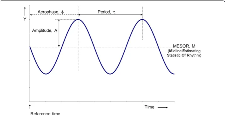
Notably in studies of circadian rhythms, it is indeed possible to assume that the period is known, being synchronized to the external 24-hour cycle. The regression model for a single component can be written as
Y tð Þ ¼MþAcos 2ð πt=τþϕÞ þe tð Þ ð1Þ
where M is the MESOR (Midline Statistic Of Rhythm, a rhythm-adjusted mean), A is the amplitude (a measure of half the extent of predictable variation within a cycle),ϕis the acrophase (a measure of the time of overall high values recurring in each cycle), τ is the period (duration of one cycle), and e(t) is the error term (Figure1).
When τcan be assumed known, using well-known trigonometric angle sum identity,
the model can be rewritten as
Y tð Þ ¼Mþβxþγzþe tð Þ ð2Þ
where
β¼Acosϕ;γ¼‐Asinϕ;x¼ cos 2ð πt=τÞ;z¼ sin 2ð πt=τÞ:
The principle underlying the least squares method is the minimization of the residual
sum of squares (RSS), that is the sum of squared differences between measurements Yi
(obtained at times ti, i = 1, 2,…, N) and the values estimated from the model at corre-sponding times
RSS¼X
i½Yi−ðM^ þβ^xiþγ^ziÞ
2 ð3Þ
Estimates for M, β, andγ are obtained by solving the normal equations, obtained by expressing that RSS is minimal when its first-order derivatives with respect to each parameter are zero.
The normal equations are X
Yi¼MNþβ
X
xiþγ
X
zi
X
Yixi¼M
X
xiþβ
X
xi2þγ
X
xizi
X
Yizi¼M
X
ziþβ
X
xiziþγ
X
zi2
ð4Þ
or in matrix form
X
Yi
X
Yixi
X
Yizi
0 B @ 1 C A¼
N Xxi
X
zi
X
xi
X
xi2
X
xizi
X
zi
X
xizi
X zi 2 0 B B @ 1 C C A M β γ 0 @ 1
Aor d¼Su ð5Þ
Estimates of M,βandγ(or vectorially, u) are thus obtained as
^
u¼S‐1d ð6Þ
Estimates for the amplitude and acrophase can be derived from the estimates of β
andγby the following relations
^
A ¼ ^β2þγ^2
1=2
^
ϕ ¼ arctan ‐^γ=^β
þKπ where K is an integer ð
7Þ
The correct value ofϕ^ is determined by taking into account the signs ofβ^andγ^. For rhythm detection, the total sum of squares (TSS) is partitioned into the sum of squares due to the regression model (MSS) and the residual sum of squares (RSS). TSS is the sum of squared differences between the data and the arithmetic mean. MSS is
the sum of squared differences between the estimated values based on the fitted model and the arithmetic mean. As noted above, RSS is the sum of squared differences be-tween the data and the estimated values from the fitted model.
TSS¼MSSþRSS or XðYi‐YÞ2¼
X
^ Yi‐Y
2
þX Yi‐Y^i
2
ð8Þ
The model is statistically significant when the model sum of squares is large relative to the residual sum of squares, as determined by the F test
F¼ðMSS=2Þ=ðRSS=ðN‐3ÞÞ ð9Þ
where 2 and N-3 are the numbers of degrees of freedom attributed to the model (k = 3 parameters –1) and to the error term (N –k). The null hypothesis (H0) that there is no rhythm (the amplitude is zero) is rejected when F > F1-α(2, N-3), whereαrelates to the chosen probability level for testing H0.
For parameter estimation, it seems reasonable to consider the MESOR (M) separately
and (β,γ) together. The 1-αconfidence interval forM is then given by^
^
Mt1‐α=2ðN‐3Þσ^
ffiffiffiffiffiffi
s‐1 11
q
ð10Þ
where s‐1
ij are the elements of S
-1 ,
^
σ ¼½RSS=ðN−3Þ1=2 ð11Þ
and tp(f ) denotes the pth probability point of Student’s t on f degrees of freedom. The covariance matrix for β^;γ^
is given by
^
σ2 s‐221 s‐231
s‐1 32 s‐331
;
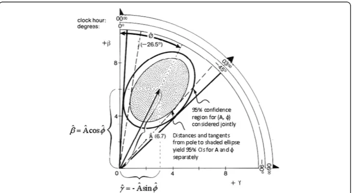
from which a 1-αconfidence region for ^β;^γ
, or equivalently forA^;ϕ^can be derived. It is based on the F-statistic used for rhythm detection, being evaluated at the estimated value ofA instead of at A = 0. The resulting equation is that of an ellipse (Figure^ 2):
X
xi‐x
ð Þ2β−^β2þ2Xx i‐x
ð Þðzi‐zÞ β‐^β
γ‐^γ
ð Þ þXðzi‐zÞ2ðγ‐^γÞ2≤2σ^2F1‐αð2;N‐3Þ ð12Þ where
X¼ X
i Xi ! =N and
Z¼ X
i
Zi !
=N
The region delineated by this ellipse represents the confidence region for the rhythm
Standard errors (SEs) forA and^ ϕ^ can also be derived from the covariance matrix for
^
β;γ^
, by using Taylor’s series expansion:
SE A^ ¼σ^ s22‐1cos2ϕ^‐2s‐231sinϕ^cosϕ^þs33‐1sin2ϕ^1=2 SE ϕ^ ¼σ^ s‐1
22sin2ϕ^þ2s‐231sinϕ^cosϕ^ þs‐331cos2ϕ^
1=2
=A^ ð13Þ
Time (clock hours)
Regression diagnostic tests
It should be noted that the P-value obtained from the F-test and the corresponding
confi-dence limits derived for M^;β^andγ^ are valid only if assumptions underlying the use of the least squares procedure are satisfied. These assumptions are (1) the model fits the data well, (2) the residuals are normally distributed, (3) the variance is homogeneous, (4) the residuals are independent, and (5) the parameters do not change over time.
Model adequacy:
Goodness of fit can be examined when replicates are available, either from multiple data collection at different timepoints or from data covering multiple cycles. RSS can then be further partitioned into the“pure error”and the“lack of fit”. An F-test compar-ing the pure error and lack of fit sums of squares provides a test of the model adequacy [44]. The pure error sum of squares (SSPE) is defined as the sum of squared differences (across all timepoints) between the data collected at a given timepoint and their re-spective arithmetic mean, whereas the sum of squares ascribed to lack of fit (SSLOF) is obtained by subtracting SSPE from RSS
SSLOF¼RSS‐SSPE SSPE¼X
i
X
lðYil–YiÞ
2 ð14Þ
withYi¼
X
lYil
=niwhere niis the number of data collected at time ti.
The appropriateness of the model is rejected if
F¼½SSLOF=ðm‐1‐2pÞ=½SSPE=ðN‐mÞ>F1‐αðm‐1‐2p;N‐mÞ ð15Þ
where m is the number of timepoints and p is the number of (cosine) components in the model (p = 1 for the single-component cosinor).
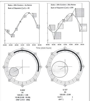
In the presence of lack of fit, adding components in the model may be considered (Figure 3).
Normality of residuals:
The rankit plot provides an attractive visual technique to test normality [44,45]. In this test, the errors (ei) are sorted by increasing order and expected values of a normal sample of size N with zero mean (rankits, zi) are calculated. If the residuals are nor-mally distributed, the regression of eion ziis a straight line. The Shapiro-Wilk test of normality can be applied for small sample sizes (N≤50) [46]. For larger sample sizes, a chi-square test of goodness of fit can be used [23] by comparing expected and observed frequencies of residuals grouped in classes.
Homogeneity of variance:
performed by fitting the model to the square of the estimated values instead of the data in order to obtain residuals rei. If
F¼ðN‐2p‐2Þr2=1‐r2>F1‐αð1;N‐2p‐2Þ ð16Þ
where r denotes the regression coefficient of reion ei, the assumption of homogeneity of variance is rejected.
Independence of residuals:
While violation of independence usually does not affect the estimate of the parameter themselves, their confidence intervals tend to be under-estimated [48]. When residuals are positively correlated, they tend to assume the same sign for long sequences. The runs test is a non-parametric test that allows to test whether sequences (runs) of posi-tive and negaposi-tive residuals occur randomly. Specifically, if successive errors are inde-pendent, there cannot be any regular sequences, either too long or too short. In other words, the number of runs cannot be too small or too large, respectively. For a given sample size, tables list limits for acceptable numbers of runs compatible with the as-sumption of independence [23,49,50].
When residuals are correlated, the data can either be low-passed filtered by averaging or decimation (using only one every k values, thereby lengthening the sampling interval from Δt to kΔt). A slightly different model can also be considered wherein the error term is replaced by an autoregressive error term [10,51,52].
Stationarity:
The problem of stationarity arises primarily in long time series, when the MESOR, amplitude, acrophase and/or period can change as a function of time. This may occur, for instance, when a person being monitored travels across time zones (e.g., from the USA to Europe). A head cold or pain can also bring about transient changes in circa-dian rhythm characteristics of variables such as body temperature, blood pressure or heart rate. Changes in period can be anticipated when time clues (environmental syn-chronizers) are removed. They are also present in the case of components with no strong environmental synchronizer. This concerns primarily non-photic cycles such as the about 1.3-year transyear and the about 5-month cis-half-year found in solar wind speed and solar flares, respectively. These components are wobbly by nature, even in
the environment. Counterparts in biology have been found, as discussed elsewhere [3,53-56]. There are several approaches available to analyze non-stationary time series, such as wavelets, short-term Fourier transforms, and gliding spectral windows comple-mented by chronobiologic serial sections, as discussed below.
For short and sparse time series, for which the cosinor method was originally devel-oped, underlying assumptions are usually valid (or at least statistical power is not suffi-cient to invalidate them). With longer and denser data, the likelihood of violating one or several underlying assumptions increases. Violation of one assumption can also re-sult in violating one or several other assumptions. For instance, when there is lack of fit, residuals tend not to be independent and may not follow a normal distribution. Confidence intervals and P-values tend to be affected more than the estimation of pa-rameters. Even when one or several underlying assumptions are violated, the informa-tion from the cosinor analysis may be of value as long as results are properly qualified. Many of the conventional methods of data analysis depend on similar assumptions, with the exception of robust non-parametric techniques [10,57-61].
Multiple-component cosinor
The single-component cosinor is easily extended to a multiple-component model (Figure 3)
Y tð Þ ¼MþX
jAjcosð2πt=τjþϕjÞ þe tð Þ;j¼1;2;…;p ð17Þ
Instead of solving a system of 3 equations in 3 unknowns, there are 2p + 1 normal equations to estimate M and p pairs of (βj,γj) or (Aj, ϕj) whenτjare assumed known. Generally, in the normal equations d = Su
d¼X
ixivYiand Su¼
X
juj
X
ixivxijfor i¼1;2;…;N;
j¼1;2;…;2pþ1;and v¼1;2;…;2pþ1
ð18Þ
where {xij} are the cos(2πti/τj) and sin(2πti/τj).
Estimates of u (M,β1,γ1,β2,γ2,…,βp,γp) are obtained as
^
u¼S‐1X’Y where S¼X’X¼ X
ixijxik
:
A confidence ellipsoid can be determined [43] from which approximate confidence
intervals can be derived for each component’s amplitude and acrophase, as outlined
above. Computations are greatly simplified in the case of equidistant data covering an integer number of cycles [45].
A multiple-component model is useful to obtain a better approximation of the
sig-nal’s waveform when it deviates from sinusoidality. For instance, a 2-component
diovascular disease risk [64].
Population-mean cosinor
When data are collected as a function of time on 3 or more individuals, the population-mean cosinor procedure renders it possible to make inferences concerning a population rhythm, provided the k individuals represent a random sample from that population. Each individual series is analyzed by the single- or multiple-component
single cosinor to yield estimates of u^¼M^i;^β1i;γ^1i;β^2i;γ^2i;…;β^pi;γ^pi;i¼1;2;…;k
n o
.
The goal is to make inferences concerning the population averages of the parameters, u*. The “*” indicates that the expectations are population averages and not averages
over the k individuals sampled. Individual vectors ui are assumed to represent a
random sample from a (2p + 1)-variate, normal population with mean u*. The within-individual variances are also assumed to be equal, so that the pooled estimate of vari-ance can be estimated as
^ σ2¼X
j nj‐ð2pþ1Þ
^ σ2
j=ðN‐ð2pþ1ÞkÞ ð19Þ
When the sample sizes for all individuals are the same or almost the same, as is often the case in hybrid designs, the population estimates are unweighted averages of the in-dividual parameters
^ u ¼X
ju^jn=k for j¼1;2;…;k and
n¼1;2;…;2pþ1 u^n¼ M^;β^1;^γ1;β^2;^γ2;…;β^p;γ^p
n o
ð20Þ
and the population amplitudes and acrophases can be estimated using the relations
^
β ¼A^cosϕ^; ^γ ¼‐A^sinϕ^
In the above conditions and assuming normality of errors and individual parameters, sample variances can be computed as
^
σ2
M¼Σj M^j−M^
2
=ðk‐1Þ; ^σ2
βn¼Σjðβ^nj−β^Þ 2
=ðk‐1Þ; ^
σ2
γn¼Σj ^γnj‐^γ
2
=ðk‐1Þ; ^σ2
Mβ1¼Σj M^j‐M^
ðβ^1j‐β^1Þ=ðk‐1Þ;
and similarly for the other cross‐products
ð21Þ
where
In the case when the population-mean cosinor can be applied separately for each trial period (p = 1), a confidence interval for M* is given by
^
M t1‐α=2ðk‐1Þσ^M=k1=2 ð22Þ
and a joint 1-αconfidence ellipse forðβ^;γ^Þconsists of all points (βz*,γz*) satisfying
ðβz‐^βÞ 2
=^σ2
β‐2rðβz‐^βÞðγz‐^γÞ=^σβσ^γþðγz‐^γÞ
2=^σ2
γ≤
2 1 ‐r2ðk‐1ÞF1‐αð2;k‐2Þ=ðk kð ‐2ÞÞ
ð23Þ
where
r¼σ^βγ=^σβσ^γ
The null hypothesis of A* = 0 is rejected if h
k kð ‐2Þ
ð Þ=ð2 kð ‐1ÞÞ
ih
1=1‐r2i β^2=^σ2β‐2rβ^^γ=^σβσ^γþγ^2=^σ2γ
h i
>F1‐αð2;k‐2Þ ð24Þ
and approximate confidence intervals forA^andϕ^can be obtained by computing the minimal and maximal distances from the pole (zero) to the error ellipse and by drawing tangents from the pole to the error ellipse, respectively (Figure 4). As for the single cosinor, closer approximate limits can also be computed [43].
Parameter tests
Test statistics have been developed to test the equality of MESORs, amplitudes and acrophases considered jointly or separately for the case of the single cosinor and the population-mean cosinor [43]. These tests can allow for a clearer interpretation of the results, for instance in a circadian experiment involving 6 timepoints 4 hours apart: Student t-tests are sometimes applied at each separate timepoint without adjustment of
amplitude and acrophase can be obtained for any trial period. This procedure, however, is valid only if there is sufficient evidence for considering this particular trial period. In the absence of such evidence, results can no longer be taken at their face value.
It has become much easier for chronobiologists to collect data over much longer spans and/or at much shorter intervals, but it has been more difficult to obtain series of equidistant data. Even for variables that are obtained with automated instrumenta-tion (such as telemetry or ambulatory blood pressure monitors), it is not uncommon to have missing data or to have additional data collected manually at times different from the scheduled times. Investigations have also extended outside the circadian realm. For these reasons, a least squares approach to time series analysis remains attractive, as long as caution is properly taken in interpreting the results.
Just as a chronogram provides useful information prior to quantitative data analysis, a view of the time structure of the data in the frequency domain can also be inform-ative. For this purpose, using the cosinor at Fourier frequencies in the range of 1/T (where T is the length of the data series) up to 1/2Δt (whereΔt is the sampling inter-val) can be viewed as no more than another macroscopic view of the data. A plot of amplitudes as a function of frequency (least squares spectrum) is equivalent to a discrete Fourier transform when data are equidistant [38].
– Large spectral peaks indicate the presence of signals and provide an approximate
estimate of their periods. This information can be used to validate anticipated components while also revealing the presence of other cycles. For rhythms that are anticipated, rhythm detection and parameter estimation can proceed as outlined above as long as P-values are adjusted for multiple testing [74]. Caution needs to be taken regarding non-anticipated cycles. The information thus gained can be used to design the next study or to examine other similar data series that could serve as replications. Additional analyses can be performed to determine the extent of stability of the unanticipated component, for instance by means of applying a chronobiologic serial section [21] or a gliding spectral window [75].
– Plotting log-amplitudes versus log-frequency provides useful information regarding
– Single spectral peaks are found only if the data cover an integer number of cycles. If this is not the case, the signal spreads over several spectral lines [10]. When this happens and the underlying signal was anticipated, it is possible to determine the period (frequency) corresponding to the maximal amplitude by applying the single cosinor procedure not only at the Fourier frequencies but at additional
intermediary frequencies as well. Whereas this may provide a clearer picture of the signal, it should be realized that the resolution in frequency (1/T) remains the same, being determined by the series length, T. Tapers such as a Hanning window [77] can be used to reduce sidelobes associated with the finite observation span, but this procedure also affects the estimation of the rhythm parameters. While a Hanning taper does not affect the location of spectral peaks in a spectrum, the width of the peak is wider and the amplitude is reduced (Figure5). It remains useful, however, for a macroscopic view of the time structure of the data.
Least squares spectra can be very helpful in exploratory analyses, but it should be re-alized that assumptions underlying the use of the single cosinor (notably independence and normality) are violated more often than not. Population-mean cosinor spectra are a useful complementary approach not prone to this limitation. This method is similar to the power spectrum obtained by smoothing the periodogram, which is more reliable for testing unknown periodicities [78], with the important difference, however, of retain-ing the phase information. The averagretain-ing (smoothretain-ing) can be done either in the frequency domain by averaging across consecutive Fourier frequencies, or in the time domain. The
Original data Data tapered with Hanning window
Partial least squares spectra
Time
Frequency
Extended linear-nonlinear cosinor
When the period is unknown, the single cosinor model (Equations 1 and 12) can no longer be linearized in its parameters as the period is in the argument of the cosine function. Starting from an initial (guess) estimate for the period, all parameters can be estimated using iterations aimed at minimizing the residual sum of squares. Marquardt [79] developed an algorithm which performs an optimum interpolation between the Taylor series and gradient methods. He also derived a way to approximate confidence intervals for all parameters, including the period [80]. For the particular case of single-component models, Bingham offers an easily understood approach [81].
For low-frequency signals, simulated annealing [82] is another suitable method that has the advantage of not requiring the specification of initial values for the periods. This approach does not perform well, however, for very sharp signals in the higher fre-quency range of the spectrum. Both simulated annealing and Marquardt’s nonlinear ap-proach performed best in distinguishing two signals with close periods sampled over less than a beat cycle, when compared to other approaches [83].
For signals with a symmetrical waveform, the nonlinear procedure can yield an ac-ceptable estimate of the fundamental period on the basis of very short records not even covering a full cycle [84]. This is not the case, however, when the waveform is asym-metrical. Simulations indicate that about 5 cycles are needed to obtain a reasonable es-timate of the period in this case, when the model fitted includes only the fundamental component. Including additional harmonic terms in the model allows the nonlinear procedure to correctly estimate the fundamental period with data covering no more than 2 cycles [84].
Analysis of non-stationary data
When data are equidistant or rendered equidistant by averaging and filling data gaps by interpolation, wavelets can be performed [85]. This approach has been useful to un-cover components not detected earlier [86]. Short-term Fourier transforms can be used to visualize changes in the spectral structure of the data as a function of time [87]. Alternatively, gliding spectral windows [75] can be computed. The method consists of
defining an interval (I) that is progressively displaced by a given increment (δt)
chart. One example relates to competing about 24.0- and 24.8-hour components coex-isting in the physiology of an apparently seleno-sensitive woman with adynamic epi-sodes recurring twice a year and lasting 2–3 months, as illustrated for systolic blood pressure in Figure 6. Another example illustrates the changing prominence of the about-weekly and about-daily rhythms in blood pressure and heart rate during the first 40 days of life of a clinically healthy boy [88]. Whereas the procedure can be performed on non-equidistant data, the interpretation of results is greatly helped when data are equidistant, as changes in sampling rate are also associated with changes in spectral structure appearing on the graph. A judicious choice of I and of the frequency range examined is important in order to minimize sidelobes. The use of a Hanning taper [77] is also helpful in this kind of exploratory analysis.
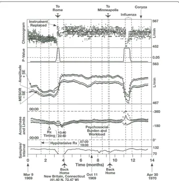
Whenever focus can be placed on a specified component with a given trial period, a chronobiologic serial section [21] can be performed. As for the gliding spectral window, an interval I is selected that is progressively displaced throughout the time series byδt increments. To data in each interval, the single-component single cosinor procedure is applied. To visualize the results, a chronogram is shown on top, followed by the se-quence of MESORs, amplitudes and acrophases as they change as a function of time, provided with a measure of uncertainty. Corresponding P-values from the zero-amplitude test and the number of data per interval are also displayed to help interpret any change in the results. This procedure has been extensively used in studies of phase shifts associated with transmeridian flights [89], as illustrated in Figure 7, and in cases when the circadian rhythm is desynchronized from 24 hours [90,91].
17 Nov 2009 6 Apr 2010 31 Aug 2010
Time (calendar date)
30.0
24.8
24.0
21.0
Period (hours)
Competing Solar-Societal vs. Lunar Pulls *
* Systolic blood pressure of JF (F, 62y). Alternating 24.0-hour synchronization and desynchronization, the latter not quite a free-run.
Amplitude (mmHg)
17.5-20.0 15.0-17.5 12.5-15.0 10.0-12.5 7.5-10.0 5.0-7.5 2.5-5.0 0.0-2.5 Episodes of
adynamic depression
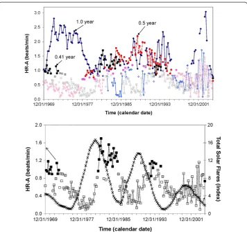
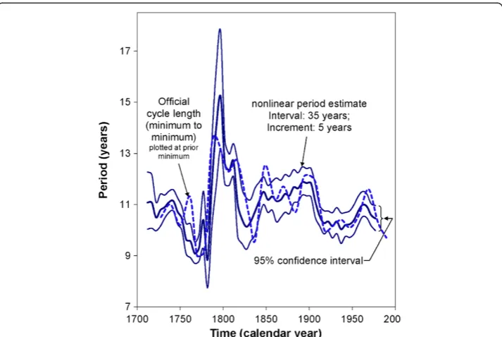
The procedure has been extended in two ways. First, a multiple-component instead of a single-component single cosinor model can be fitted in each interval. This proced-ure has been used for instance to illustrate that the prominence of an about 5-month component of heart rate self-measured over 4 decades by a clinically healthy man follows the about 11-year change in solar flares in which this component had been doc-umented [92]. In this analysis, the 5-month component was fitted together with 1.0-and 0.5-year components over a 4-year interval displaced by 0.2-year increments [93]. Figure 8 illustrates the changing prominence of the three components as a function of time. An about 11-year cycle in the prominence of the about 5-month component is highlighted. Second, a nonlinear model can be fitted in each interval and the period displayed as a function of time with its 95% confidence interval. This approach was
used to illustrate the great variability in the length of the about 11-year solar activity cycle, Figure 9 [94].
Discussion and conclusion
field of chronomics which aims at mapping broad time structures from the high-frequency brain waves to the multi-decadal cycles characterizing space-terrestrial wea-ther influencing human physiology and pathology [3,104].
Despite its simplicity, some reluctance remains for some investigators to use the cosi-nor for estimating rhythm parameters or for considering more than a single test time in designing experiments. Too many studies still rely on testing only at a fixed time of day (to control for the circadian variation) or at most at two times 12 hours apart, ig-noring the possibility that the two selected timepoints may be at the midline crossings rather than at the peak and trough where differences are maximal. As discussed else-where, such practice can be misleading in missing an existing difference or even in finding a difference in mean when none exists [15-17]. Computing day-night differ-ences in lieu of an amplitude and acrophase is also widely done to interpret
ambula-tory blood pressure monitoring records in terms of “dipping” [105], despite the
documentation in several outcome studies of the superiority of a chronobiological approach [106,107].
To some extent, this status quo may be accounted for by the lack of dissemination of computer software offering chronobiologists tools for time series analysis applicable to non-equidistant data. This situation is slowly changing, however. Personal computers have become more powerful and statistical packages have become more readily avail-able for relatively easy use by investigators not necessarily versed in all statistical details underlying the programs included in the software packages. While professional statis-tical software packages remain somewhat expensive for individual users, several open-source packages (such as Octave and R) offer an attractive alternative, notably since
some are platform-independent, running on PCs, Macs or Linux systems [108]. Pro-grammers have taken advantage of the tools available in these packages to write code to perform analytical tasks of interest to chronobiologists. Perhaps the most compre-hensive package is that developed by Oehlert and Bingham [109], offering a large array of procedures that can be applied by writing minimal coding instructions to call the different macros. Selected programs used in chronobiology have long been offered on the website of Refinetti [110], with clear instructions on how to run the programs. While not open-source, the Expert Soft Technologie website [111] also offers an array of cosinor-based and other procedures, including techniques for the study of non-stationary signals. These programs have been used in the study of shift-workers [112].
In summary, selected methods for the study of biologic time series have been reviewed and their relative merits have been discussed in the light of underlying assumptions. Some illustrative applications have also been mentioned. When the choice of a model is justified, and it is functional and explicative, quantitative methods of data analysis are extremely valuable to specify the model and obtain estimates of its parameters. Even when under-lying assumptions are not fully met, point estimates of the parameters can be very useful. More caution is needed, however, in deciding whether P-values and confidence intervals are trustworthy, since violation of underlying assumptions tends to yield results that are too liberal. Once this limitation is taken into consideration, data analysis methods as described herein constitute extremely valuable tools for research in chronobiology and chronomics.
Competing interests
The author declares that she has no competing interests.
Acknowledgment
Dedicated to the memory of Franz Halberg who developed the cosinor method.
Support
Halberg Chronobiology Fund, University of Minnesota Supercomputing Institute.
Received: 27 January 2014 Accepted: 18 March 2014 Published: 11 April 2014
References
1. Halberg F:Temporal coordination of physiologic function.Cold Spr Harb Symp quant Biol1960,25:289–310. 2. Halberg F, Tong YL, Johnson EA:Circadian System Phase–An Aspect of Temporal Morphology; Procedures
and Illustrative Examples.InProc. International Congress of Anatomists. The Cellular Aspects of Biorhythms, Symposium on Biorhythms.Edited by Mayersbach HV. New York: Springer-Verlag; 1967:20–48.
3. Halberg F, Cornelissen G, Katinas GS, Hillman D, Otsuka K, Watanabe Y, Wu J, Halberg F, Halberg J, Sampson M, Schwartzkopff O, Halberg E:Many rhythms are control information for whatever we do: an autobiography. Folia anthropologica2012,12:5–134.
4. Halberg F, Visscher MB:Regular diurnal physiological variation in eosinophil levels in five stocks of mice. Proc Soc exp Biol (N.Y.)1950,75:846–847.
5. Halberg F, Visscher MB, Bittner JJ:Relation of visual factors to eosinophil rhythm in mice.Amer J Physiol1954, 179:229–235.
6. Halberg F, Visscher MB, Bittner JJ:Eosinophil rhythm in mice: Range of occurrence; effects of illumination, feeding and adrenalectomy.Amer J Physiol1953,174:109–122.
7. Haus E, Cornelissen G, Halberg F:Introduction to chronobiology.InChronobiology: Principles and Applications to Shifts in Schedules.Edited by Scheving LE, Halberg F. Alphen aan den Rijn, The Netherlands: Sijthoff and Noordhoff; 1980:1–32.
8. Halberg F, Cornelissen G, Gumarova L, Halberg F, Ulmer W, Hillman D, Siegelova J, Watanabe Y, Hong S, Otsuka K, Wu J, Lee JY, Schwartzkopff O, Wendt H:Integrated and as-one-goes analyzed physical, biospheric and noetic monitoring: Preventing personal disasters by self-surveillance may help understand natural cataclysms: a chronou-sphere (chrono-noöchronou-sphere).London: SWB International Publishing House. in press.
9. Halberg E, Halberg F:Chronobiologic study design in everyday life, clinic and laboratory.Chronobiologia1980, 7:95–120.
Buckley J, Mandel J, Schuman L, Haus E, Lakatua D, Sackett L, Berg H, Wendt HW, Kawasaki T, Ueno M, Uezono K, Matsuoka M, Omae T, Tarquini B, Cagnoni M, Garcia Sainz M, Perez Vega E, Wilson D, Griffiths K, Donati L, Tatti P, Vasta M, Locatelli I, Camagna A, Lauro R, Tritsch G, Wetterberg L:International geographic studies of oncological interest on chronobiological variables.InNeoplasms—Comparative Pathology of Growth in Animals, Plants and Man.Edited by Kaiser H. Baltimore: Williams and Wilkins; 1981:553–596.
19. Halberg F, Guillaume F, Sanchez de la Peña S, Cavallini M, Cornelissen G:Cephalo-adrenal interactions in the broader context of pragmatic and theoretical rhythm models.Chronobiologia1986,13:137–154. 20. Jozsa R, Halberg F, Cornelissen G, Zeman M, Kazsaki J, Csernus V, Katinas GS, Wendt HW, Schwartzkopff O,
Stebelova K, Dulkova K, Chibisov SM, Engebretson M, Pan W, Bubenik GA, Nagy G, Herold M, Hardeland R, Hüther G, Pöggeler B, Tarquini R, Perfetto F, Salti R, Olah A, Csokas N, Delmore P, Otsuka K, Bakken EE, Allen J, Amory-Mazaudier C:Chronomics, neuroendocrine feedsidewards and the recording and consulting of nowcasts forecasts of geomagnetics.Biomed Pharmacother2005,59(Suppl 1):S24–S30.
21. Halberg F, Carandente F, Cornelissen G, Katinas GS:Glossary of chronobiology.Chronobiologia1977,4(1):189. 22. Watanabe Y, Halberg F, Otsuka K, Cornelissen G:Toward a personalized chronotherapy of high blood pressure
and a circadian overswing.Clin Exp Hypertens2013,35:257–266. 23. Sokal RR, Rohlf FJ:Biometry.secondth edition. Freeman & Co.; 1981.
24. Halberg F, Visscher MB, Flink EB, Berge K, Bock F:Diurnal rhythmic changes in blood eosinophil levels in health and in certain diseases.J Lancet1951,71:312–319.
25. Halberg F, Cornelissen G, Katinas G, Syutkina EV, Sothern RB, Zaslavskaya R, Halberg F, Watanabe Y, Schwartzkopff O, Otsuka K, Tarquini R, Perfetto P, Siegelova J:Transdisciplinary unifying implications of circadian findings in the 1950s.J Circadian Rhythms2003,1(2):61.
26. Cornelissen G, Halberg F:Chronomedicine.InEncyclopedia of Biostatistics.2nd edition. Edited by Armitage P, Colton T. Chichester, UK: John Wiley & Sons Ltd; 2005:796–812.
27. Powell EW, Pasley JN, Scheving LE, Halberg F:Amplitude-reduction and acrophase-advance of circadian mitotic rhythm in corneal epithelium of mice with bilaterally lesioned suprachiasmatic nuclei.Anat Rec1980, 197:277–281.
28. Cornelissen G, Halberg F:Introduction to Chronobiology.Minneapolis, MN: Medtronic Chronobiology Seminar #7; 1994:52. Library of Congress Catalog Card #94-060580.
29. Hillman D, Fernández JR, Cornelissen G, Berry DA, Halberg J, Halberg F:Bounded limits and statistical inference in chronobiometry.Prog Clin Biol Res1990,341B:417–428.
30. Halberg F:Chronobiology.Annu Rev Physiol1969,31:675–725.
31. Halberg F, Johnson EA, Nelson W, Runge W, Sothern R:Autorhythmometry–procedures for physiologic self-measurements and their analysis.Physiol Tchr1972,1:1–11.
32. Halberg F:Chronobiology: methodological problems.Acta med rom1980,18:399–440.
33. Halberg F, Panofsky H:I: Thermo-variance spectra; method and clinical illustrations.Exp Med Surg1961,19:284–309. 34. Panofsky H, Halberg F:II. Thermo-variance spectra; simplified computational example and other methodology.
Exp Med Surg1961,19:323–338.
35. Marquardt DW, Acuff SK:Direct quadratic spectrum estimation from unequally spaced data.InApplied time series analysis.Edited by Anderson OD, Perryman MR. North-Holland: North-Holland Publ. Co; 1982:199–227. 36. Brillinger D, Fienberg S, Gani J, Hartigan J, Krickeberg K (Eds):Time Series Analysis of Irregularly Observed Data, vol.
25.New York, Berlin, Heidelberg, Tokyo: Springer-Verlag; 1984.
37. Brillinger D, Fienberg S, Gani J, Hartigan J, Krickeberg K (Eds):Robust and Nonlinear Time Series Analysis, vol. 26. New York, Berlin, Heidelberg, Tokyo: Springer-Verlag; 1984.
38. Bloomfield P:Fourier Analysis of Time Series: An Introduction.New York: Wiley; 1976.
39. Reinberg A, Halberg F:Circadian chronopharmacology.Annu Rev Pharmacol1971,2:455–492.
40. Haus E, Halberg F, Kühl JFW, Lakatua DJ:Chronopharmacology in animals.Chronobiologia1974,1(Suppl. 1):122–156. 41. Halberg F, Haus E, Nelson W, Sothern R:Chronopharmacology, chronodietetics and eventually clinical
chronotherapy.Nova Acta leopold1977,46:307–366.
42. Reinberg A, Halberg F:Chronopharmacology.Oxford/New York: Pergamon Press; 1979.
43. Bingham C, Arbogast B, Cornelissen Guillaume G, Lee JK, Halberg F:Inferential statistical methods for estimating and comparing cosinor parameters.Chronobiologia1982,9:397–439.
44. Weisberg S:Applied Linear Regression.New York: J Wiley & Sons; 1980. 45. Bliss CI:Statistics in Biology, Volume 1.New York: McGraw Hill; 1967.
46. Shapiro SS, Wilk MB:An analysis of variance test for normality (complete samples).Biometrika1965,52:591–611. 47. Draper NR, Smith H:Applied Regression Analysis, Second Edition.New York: Wiley & Sons; 1981.
50. Conover WJ:Practical Nonparametric Statistics, Second Edition.New York: Wiley & Sons; 1980. 51. Cornelissen Guillaume G, Halberg F, Fanning R, Kanabrocki EL, Scheving LE, Pauly JE, Redmond DP,
Carandente F:Analysis of circadian rhythms in human rectal temperature and motor activity in dense and short series with correlated residuals.InBiomedical Thermology.Edited by Gautherie M, Albert E. New York: Alan R. Liss; 1982:167–184.
52. Dunstan FDJ, Barham S, Kemp KW, Nix ABJ, Rowlands RJ, Wilson DW, Phillips MJ, Griffiths K:A feasibility study for early detection of breast cancer using breast skin temperature rhythms.Statistician1982,31:37–52. 53. Halberg F, Cornelissen G, Sothern RB, Hillman D, Watanabe Y, Haus E, Schwartzkopff O, Best WR:Decadal cycles
in the human cardiovascular system.World Heart J2012,4:263–287.
54. Halberg F, Powell D, Otsuka K, Watanabe Y, Beaty LA, Rosch P, Czaplicki J, Hillman D, Schwartzkopff O,
Cornelissen G:Diagnosing vascular variability anomalies, not only MESOR-hypertension.Am J Physiol Heart Circ Physiol2013,305:H279–H294.
55. Cornelissen G, Otsuka K, Halberg F:Remove and Replace for a Scrutiny of Space Weather and Human Affairs. InInt. Conf., Space Weather Effects in Humans: In Space and on Earth.Edited by Grigoriev AI, Zeleny LM. Moscow, Russia: Space Res Inst; 2013:508–538.
56. Cornelissen G, Watanabe Y, Otsuka K, Halberg F:Influences of Space and Terrestrial Weather on Human Physiology and Pathology.InBioelectromagnetic and Subtle Energy Medicine.Edited by Rosch P. Russia: CRC Press. in press. 57. Narula SC, Saldiva PH, Andre CD, Elian SN, Ferreira AF, Capelozzi V:The minimum sum of absolute errors
regression: a robust alternative to the least squares regression.Stat Med1999,18:1401–1417.
58. Ahdesmaki M, Lahdesmaki H, Gracey A, Shmulevich L, Yli-Harja O:Robust regression for periodicity detection in non-uniformly sampled time-course gene expression data.BMC Bioinforma2007,8:233.
59. Blume JD, Su L, Olveda RM, McGarvey ST:Statistical evidence for GLM regression parameters: a robust likelihood approach.Stat Med2007,26:2919–2936.
60. Pires AM, Rodrigues IM:Multiple linear regression with some correlated errors: classical and robust methods. Stat Med2007,26:2901–2918.
61. Anderson R:Modern Methods for Robust Regression.Sage Publications, Inc.: University of Toronto; 2008. 62. Cornelissen G, Otsuka K, Halberg F:Blood pressure and heart rate chronome mapping: a complement to the
human genome initiative.InChronocardiology and Chronomedicine: Humans in Time and Cosmos.Edited by Otsuka K, Cornelissen G, Halberg F. Tokyo: Life Science Publishing; 1993:16–48.
63. Cornelissen G, Halberg F, Bakken EE, Singh RB, Otsuka K, Tomlinson B, Delcourt A, Toussaint G, Bathina S,
Schwartzkopff O, Wang ZR, Tarquini R, Perfetto F, Pantaleoni GC, Jozsa R, Delmore PA, Nolley E:100 or 30 years after Janeway or Bartter, Healthwatch helps avoid“flying blind”.Biomed Pharmacother2004,58(Suppl 1):S69–S86. 64. Halberg F, Cornelissen G, Otsuka K, Siegelova J, Fiser B, Dusek J, Homolka P, Sanchez DelaPena S, Singh RB,
BIOCOS project:Extended consensus on means and need to detect vascular variability disorders (VVDs) and vascular variability syndromes (VVSs).World Heart J2010,2:279–305.
65. Cornélissen G:Instrumentation and data analysis methods needed for blood pressure monitoring in chronobiology.InChronobiotechnology and Chronobiological Engineering.Edited by Scheving LE, Halberg F, Ehret CF. Dordrecht, The Netherlands: Martinus Nijhoff; 1987:241–261.
66. Halberg E, Halberg F, Shankaraiah K:Plexo-serial linear-nonlinear rhythmometry of blood pressure, pulse and motor activity by a couple in their sixties.Chronobiologia1981,8:351–366.
67. Cornelissen G, Halberg F, Otsuka K, Singh RB:Separate cardiovascular disease risks: circadian hyper-amplitude-tension (CHAT) and an elevated pulse pressure.World Heart J2008,1:223–232.
68. Otsuka K, Cornelissen G, Halberg F, Oehlert G:Excessive circadian amplitude of blood pressure increases risk of ischemic stroke and nephropathy.J Med Eng Technol1997,21:23–30.
69. Chen CH, Cornelissen G, Halberg F, Fiser B:Left ventricular mass index as“outcome”related to circadian blood pressure characteristics.Scr Med (Brno)1998,71:183–189.
70. Müller-Bohn T, Cornelissen G, Halhuber M, Schwartzkopff O, Halberg F:CHAT und Schlaganfall.Deutsche Apotheker Zeitung2002,142:366–370.
71. Schaffer E, Cornelissen G, Rhodus N, Halhuber M, Watanabe Y, Halberg F:Blood pressure outcomes of dental patients screened chronobiologically: a seven-year follow-up.JADA2001,132:891–899.
72. Cornelissen G, Siegelova J, Watanabe Y, Otsuka K, Halberg F:Chronobiologically-interpreted ABPM reveals another vascular variability anomaly (VVA): excessive pulse pressure product (PPP)–updated conference report.World Heart J2012,4:237–245.
73. Cornelissen G, Halberg F, Burioka N, Perfetto F, Tarquini R, Bakken EE:Do plasma melatonin concentrations decline with age?Am J Med2000,109:343–344.
74. Bonferroni CE:Teoria statistica delle classi e calcolo delle probabilità.Pubblicazioni del R Istituto Superiore di Scienze Economiche e Commerciali di Firenze1936,8:3–62.
75. Nintcheu-Fata S, Cornelissen G, Katinas G, Halberg F, Fiser B, Siegelova J, Masek M, Dusek J:Software for contour maps of moving least-squares spectra.Scr Med (Brno)2003,76:279–283.
76. Otsuka K, Cornelissen G, Halberg F:Age, gender and fractal scaling in heart rate variability.Clin Sci1997, 93:299–308.
77. Nuttall AH:Some Windows with Very Good Sidelobe Behavior.IEEE Trans Acoustics Speech Signal Process1981, 29:84–91.
78. Bendat JS, Piersol AG:Random Data-Analysis and Measurement Procedures.New York: Wiley Interscience; 1971. 79. Marquardt DW:An algorithm for least squares estimation of nonlinear parameters.J Soc Indust Appl Math
1963,11:431–441.
80. Marquardt DW:Least Squares Estimation of Nonlinear Parameters, IBM share library distribution No. 309401; 1966. 81. Bingham C, Cornelissen G, Halberg E, Halberg F:Testing period for single cosinor: extent of human 24-h
cardiovascular“synchronization”on ordinary routine.Chronobiologia1984,11:263–274.
flights and aging.InChronobiology: Principles and Applications to Shifts in Schedules.Edited by Scheving LE, Halberg F. Alphen aan den Rijn, The Netherlands: Sijthoff and Noordhoff; 1980:371–392.
90. Sanchez de la Peña S, Halberg F, Galvagno A, Montalbini M, Follini S, Wu J, Degioanni J, Kutyna F, Hillman DC, Kawabata Y, Cornelissen G:Circadian and Circaseptan (about-7-day) Free-Running Physiologic Rhythms of a Woman in Social Isolation.InProc. 2nd Ann. IEEE Symp. on Computer-Based Medical Systems.Washington DC: Computer Society Press; 1989:273–278.
91. Halberg F, Cornelissen G, Hillman D, Ilyia E, Cegielski N, El-Khoury M, Finley J, Thomas F, Brandes V, Kino T, Papadoupoulou A, Chrousos GP, Costella JF, Mikulecky M:Multiple circadian periods in a lady with recurring episodes of adynamic depression: case report. InNoninvasive Methods in Cardiology.Edited by Halberg F, Kenner T, Fiser B, Siegelova J. Brno, Czech Republic: Faculty of Medicine, Masaryk University; 2011:45–67. 92. Rieger A, Share GH, Forrest DJ, Kanbach G, Reppin C, Chupp EL:A 154-day periodicity in the occurrence of hard
solar flares?Nature1984,312:623–625.
93. Cornelissen G, Halberg F, Sothern RB, Hillman DC, Siegelova J:Blood pressure, heart rate and melatonin cycles synchronization with the season, earth magnetism and solar flares.Scr Med2010,83:16–32.
94. Cornelissen G, Halberg F, Gheonjian L, Paatashvili T, Faraone P, Watanabe Y, Otsuka K, Sothern RB, Breus T, Baevsky R, Engebretson M, Schröder W:Schwabe’s ~10.5- and Hale’s ~21-Year Cycles in Human Pathology and Physiology.InLong- and Short-Term Variability in Sun’s History and Global Change.Edited by Schröder W. Bremen: Science Edition; 2000:79–88.
95. Box GEP, Jenkins GM:Time Series Analysis: Forecasting and Control, Holden-Day; 1970. 96. Mills TC:Time Series Techniques for Economists.Cambridge: Cambridge University Press; 1990.
97. Percival DB, Walden AT:Spectral Analysis for Physical Applications.Cambridge: Cambridge University Press; 1993. 98. Anderson N:On the calculation of filter coefficients for maximum entropy spectral analysis.Geophysics1974,
39:69–72.
99. Burg JP:Maximum Entropy Spectral Analysis.Oklahoma City: Paper presented at the 37th Annual Int. Meeting Soc. Of Explo. Geophy; 1967.
100. Enright JT:The search for rhythmicity in biological time-series.J Theor Biol1965,8:426–468.
101. Lomb NR:Least-squares frequency analysis of unequally spaced data.Astrophysics Space Sci1976,39:447–462. 102. Scargle JD:Studies in astronomical time series analysis. II - Statistical aspects of spectral analysis of unevenly
spaced data.Astrophysical J1982,263:835–853.
103. Van Dongen HPA, Olofse E, Van Hartevelt JH, Kruyt EW:Searching for Biological Rhythms: Peak Detection in the Periodogram of Unequally Spaced Data.J Biol Rhythm1999,14:617–620.
104. Halberg F, Cornelissen G, Katinas G, Hillman D, Schwartzkopff O:Season’s Appreciations 2000: Chronomics complement, among many other fields, genomics and proteomics.Neuroendocrinol Lett2001,22:53–73. 105. Verdecchia P, Schillaci G, Guerrieri M, Gatteschi C, Benemio G, Boldrini F, Porcellati C:Circadian blood pressure
changes and left ventricular hypertrophy in essential hypertension.Circulation1990,81:528–536. 106. Al-Abdulgader AA, Cornelissen G, Halberg F:Vascular Variability Disorders in the Middle East: case reports.
World Heart J2010,2:261–277.
107. Cornelissen G, Halberg F, Otsuka K, Singh RB, Chen CH:Chronobiology predicts actual and proxy outcomes when dipping fails.Hypertension2007,49:237–239.
108. Lee-Gierke C:Analysis of Rhythms Using R: Introducing Chronomics Analysis Toolkit (CAT).Minnesota: A Master’s Thesis Submitted to the Graduate Faculty of the University of Minnesota; 2013.
109. Oehlert GW, Bingham C:MacAnova. A Program for Statistical Analysis and Matrix Algebra.http://www.stat.umn.edu/ macanova/.
110. Refinetti R:Circadian Software.http://www.circadian.org/softwar.html.
111. Gouthiere L, Mauvieux B:Etapes essentielles dans l’analyse des rythmes: qualité des données expérimentales, recherche de périodes par analyses spectrales de principes divers, modélisation.http://www.euroestech.net/resources/eedadr.pdf. 112. Gouthiere L, Mauvieux B, Davenne D, Waterhouse J:Complementary methodology in the analysis of rhythmic
data, using examples from a complex situation, the rhythmicity of temperature in night shift workers. Biol Rhythm Res2005,36:177–193.
doi:10.1186/1742-4682-11-16