Atmos. Meas. Tech., 4, 1361–1381, 2011 www.atmos-meas-tech.net/4/1361/2011/ doi:10.5194/amt-4-1361-2011
© Author(s) 2011. CC Attribution 3.0 License.
Atmospheric
Measurement
Techniques
Effects of ice particles shattering on the 2D-S probe
R. P. Lawson
SPEC Incorporated, 3022 Sterling Circle, Suite 200, Boulder, Colorado, 80301, USA Received: 2 February 2011 – Published in Atmos. Meas. Tech. Discuss.: 9 February 2011 Revised: 10 June 2011 – Accepted: 15 June 2011 – Published: 5 July 2011
Abstract. Recently, considerable attention has been focused on the issue of large ice particles shattering on the inlets and tips of cloud particle probes, which produces copious ice particles that can be mistakenly measured as real ice parti-cles. Currently two approaches are being used to mitigate the problem: (1) Based on recent high-speed video in icing tun-nels, probe tips have been designed that reduce the number of shattered particles that reach the probe sample volume, and (2) Post processing techniques such as image processing and using the arrival time of each individual particle. This paper focuses on exposing suspected errors in measurements of ice particle size distributions due to shattering, and evaluation of the two techniques used to reduce the errors. Data from 2D-S probes constitute the primary source of the investiga-tion, however, when available comparisons with 2D-C and CIP measurements are also included. Korolev et al. (2010b) report results from a recent field campaign (AIIE) and con-clude that modified probe tips are more effective than an ar-rival time algorithm when applied to 2D-C and CIP measure-ments. Analysis of 2D-S data from the AIIE and SPARTI-CUS field campaigns shows that modified probe tips signifi-cantly reduce the number of shattered particles, but that a par-ticle arrival time algorithm is more effective than the probe tips designed to reduce shattering. A large dataset of 2D-S measurements with and without modified probe tips was not available from the AIEE and SPARTICUS field campaigns. Instead, measurements in regions with large ice particles are presented to show that shattering on the 2D-S with modified probe tips produces large quantities of small particles that are likely produced by shattering. Also, when an arrival time algorithm is applied to the 2D-S data, the results show that it is more effective than the modified probe tips in reduc-ing the number of small (shattered) particles. Recent results
Correspondence to: R. P. Lawson ([email protected])
from SPARTICUS and MACPEX show that 2D-S ice particle concentration measurements are more consistent with physi-cal arguments and numeriphysi-cal simulations than measurements with older cloud probes from previous field campaigns. The analysis techniques in this paper can also be used to estimate an upper bound for the effects of shattering. For example, the additional spurious concentration of small ice particles can be measured as a function of the mass concentration of large ice particles. The analysis provides estimates of upper bounds on the concentration of natural ice, and on the re-maining concentration of shattered ice particles after appli-cation of the post-processing techniques. However, a com-prehensive investigation of shattering is required to quantify effects that arise from the multiple degrees of freedom asso-ciated with this process, including different cloud environ-ments, probe geometries, airspeed, angle of attack, particle size and type.
1 Introduction
1362 R. P. Lawson: Effects of ice particles shattering on the 2D-S probe equivalent to a spacing that is less than about 2 cm are
con-sidered artifacts, and are removed. Cooper (1978) introduced the arrival time approach, which was later refined by Field et al. (2003, 2006), Korolev and Isaac (2005) and Baker et al. (2009). The work presented by Baker et al. (2009) consid-ers removal of splashing raindrops, which closely resembles shattered ice particles.
While the issue surrounding ice particles shattering on the inlets and tips of optical particle probes (hereafter referred to simply as “shattering”) has been known since the 1970’s, it has only been recently that the magnitude of the effect has been brought to the attention of the cloud physics commu-nity. Advances in high-speed digital videography and cloud particle probes have provided new insights into the ing process. High-speed videography of ice particles shatter-ing on probe tips in the Cox & Company Incoporated icshatter-ing wind tunnel by the National Aeronautics and Space Admin-istration (NASA) Glenn Research Center (GRC) and Envi-ronment Canada (EC) showed some remarkable results. Ko-rolev et al. (2010a) shows digital videography of ice particles a few hundreds of micrometers in size shattering on probe tips, with small ice particles bouncing several mm upstream into the 100 m s−1 airflow, and then traversing up to 3 cm across the airflow into the probe sample volume.
Advances in the electro-optics of linear-array cloud par-ticle probes over the past four decades have provided new insights into measurements of cloud particle size distribu-tions. To summarize, the 2D-C probe (Knollenberg, 1970) has 25-µm pixels with 32 photodiodes that are strobed at 5 MHz. The cloud imaging probe (CIP), designed and built by Droplet Measuring Technology (DMT) in the late 1990’s (Baumgardner et al., 2001), has 64 photodiodes, 25-µm pix-els and is strobed at 8 MHz. The 2D-S probe has 128 pho-todiodes, 10-µm pixels and is strobed at 20 Mhz. Lawson et al. (2006a) show laboratory results that demonstrate the ability of the 2D-S to image an 8-µm pixel fiber at speeds exceeding 200 m s−1. In comparison, limitations of the time response of the photodiode array and front end amplifier in CIP and 2D-C probes may result in under sizing of small (e.g., <∼100 µm) particles. Lawson et al. (2006a) showed measurements that suggest that the 2D-C does not image particles <∼125 µm at an airspeed of 103 m s−1. Strapp et al. (2001) report on the efficiency of a 2D-C probe to detect 60-µm opaque circular dots on before a clear disk spinning at 100 m s−1. The results show that the depth of field (DoF) of the 2D-C probe reduces from about 75 mm to 10 mm when the disk speed increases from 10 to 100 m s−1,
and that 80 % of the 60- µm spots are detected exactly at the center of the DoF, with the percentage of detected dots (in-cluding zero area images) decreasing to about 10 % within 3 mm of the center of DoF. Recent measurements show that a newer version of the CIP is capable of imaging 50- µm drops at 150 m s−1, but that performance degrades at higher airspeeds (Lawson et al., 2010). These results suggest that the time response, and therefore the ability of the 2D-C and
CIP probes to image small particles, have improved over the past two decades. However, there is no evidence to date that shows that the 2D-C and CIP probes can detect particles less than 50 µm in size at jet aircraft speeds. On the other hand, the 2D-S probe has demonstrated the ability to image 10- µm particles at jet aircraft speeds.1
This paper is focused on exposing suspected errors in mea-surements of ice particle size distributions due to shattering, and evaluation of techniques used to reduce these errors. It is not intended to be a comparison of the relative performance of various imaging probes. However, Korolev et al. (2010b) recently evaluated shattering effects on 2D-C and CIP probes and reported that specially modified tips were more effective than an arrival time algorithm in reducing the effects of shat-tering. In this paper it is seen that, after evaluating limited data collected by two 2D-S probes, one with and one with-out modified tips, we find a different result; i.e., an arrival time algorithm is more effective in reducing the apparent ef-fects of shattering than modified tips. The limited dataset with and without modified probe tips is not intended to pro-vide guidance for quantitative assessment of shattering on the 2D-S probe. However, the data do show that, contrary to the results presented for 2D-C and CIP probes in Korolev et al. (2010b), the 2D-S probe with modified tips detects shat-tered particles in significant quantities. This may be due to the improved time response and size resolution of the 2D-S probe, or other factors, such as the probe tip design. Regard-less, the results show that the arrival time algorithm is more effective than the modified probe tips in reducing the num-ber of small (shattered) particles in these regions of large ice particles.
We concentrate on 2D-S measurements, which themselves contain uncertainties, some known and others that will likely be exposed over time. However, when available we have in-cluded comparable 2D-C and CIP measurements. A com-parison of 2D-S and historical measurements also leads to implications regarding how uncertainties may impact cloud particle data in archives.
2 Comparison of measurements from a 2D-S and historical measurements
Historical aircraft measurements of ice particle size distri-butions using optical probes in deep stratus cloud systems, such as thick cirrus, have generally revealed a vertical profile
1The electronics in some 2D-C and CIP probes have recently
R. P. Lawson: Effects of ice particles shattering on the 2D-S probe 1363
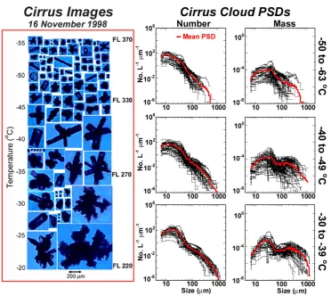
Figure 1. Example of (left) vertical profile of CPI images in a deep orographically generated
cirrus, and (middle and right panels) number and mass particle size distributions for three temperature ranges generated from 102 horizontal legs in cirrus, where average size distribution distributions are shown in red. Small end of the size distributions are based on measurements from FSSP and large end from 2D-C probe, with CPI data scaled to fit in between. Adapted from Lawson et al. (2006b).
In contrast to the vertical distribution of small ice particles seen in Fig. 1, the
measurements in Fig. 2 were collected using a 2D-S probe in a deep cirrus cloud investigated
from 193630 – 195900 UTC on 10 February 2010 during the Small PARTIcles in CirrUS (SPARTICUS) project. This example was chosen from the SPARTICUS dataset because it shows high (2.7 cm-3) concentrations of small ice near cloud top (and the CPI images reveal
nearly all small ice), but only 44 L-1 near cloud base, including bullet rosettes with sizes of
hundreds of microns. A comparison of the size distributions in Figs. 1 and 2 shows that both
the concentration and mass distributions have similar shapes near cloud top where there were few large ice particles. However, lower in the cloud where there are higher concentrations of large ice particles, the mode of the mass distribution in Fig. 1 peaks between 10 and 100 m,
whereas the mass mode peaks between 100 and 500 m in Fig. 2. The much smaller mass
Fig. 1. Example of (left) vertical profile of CPI images in a deep orographically generated cirrus, and (middle and right panels) number and mass particle size distributions for three temperature ranges generated from 102 horizontal legs in cirrus, where average size distributions are shown in red. Small end of the size distributions are based on measurements from FSSP and large end from 2D-C probe, with CPI data scaled to fit in between. Adapted from Lawson et al. (2006b).
where small ice particles exist and typically dominate the size distribution throughout the depth of cloud (e.g., Law-son et al., 2006b). This is contrary to conventional thinking, which suggests that smaller particles will nucleate in higher concentrations at cold temperatures near cloud top and sub-sequently sublimate and disappear, grow via vapor diffusion, or aggregate into larger ice particles as they fall toward cloud base.
To help visualize the effects of shattering on archival data, we show two examples of vertical profiles of ice particle size distributions collected in relatively deep cirrus clouds. The first example shows average ice particle size distribu-tions using older cloud particle probes that are believed to be subject to errors from shattering. The second example shows data from the 2D-S probe, which used modified probe tips based on the Korolev design technique and particle ar-rival times (Baker et al. 2009) to remove shattered ice in post processing. Figure 1 shows an example from Law-son et al. (2006b) of particle size distributions and num-ber concentrations based on multiple penetrations of cirrus clouds. Composite size distributions were put together using
measurements from a forward scattering spectrometer probe (FSSP), a cloud particle imager (CPI) and a 2D-C probe. The FSSP was used to establish the small particle end of the size distribution (generally less than about 30 µm) and the 2D-C established the large end. CPI data were scaled to merge with the FSSP and 2D-C measurements (see Lawson et al., 2006b for details).
A combination of gravity waves and homogenous nucle-ation at these cold temperatures is a possible theoretical ex-planation for the relatively high (846 l−1)average ice
con-centration near cloud top in Fig. 1 (K¨archer and Str¨om, 2003; Jensen et al., 2009). Some investigators have reported even higher (>1 cm−3) ice concentrations in regions where the maximum particle size is about 100 µm (Gayet et al., 2002; K¨archer and Str¨om, 2003; Lawson et al., 2006b). Shattering is not thought to be a major contributor to ice concentration in this situation. However, the high (2.17 cm−3)average ice concentration near cloud base in Fig. 1 cannot be explained theoretically.
1364 R. P. Lawson: Effects of ice particles shattering on the 2D-S probe the FSSP was very sensitive to shattering, and that the
shat-tered artifacts could significantly increase the small particle concentration. Most of the measurements that suggest high concentrations of small ice in regions with large ice (i.e.,>
a few hundreds of microns) have been reported using (or in the case of the CPI scaled by) a scattering probe such as the FSSP (e.g., Fig. 1).
In contrast to the vertical distribution of small ice parti-cles seen in Fig. 1, the measurements in Fig. 2 were col-lected using a 2D-S probe in a deep cirrus cloud investigated from 19:36:30–19:59:00 UTC on 10 February 2010 during the Small PARTIcles in CirrUS (SPARTICUS) project. This example was chosen from the SPARTICUS dataset because it shows high (2.7 cm−3)concentrations of small ice near cloud
top (and the CPI images reveal nearly all small ice), but only 44 l−1near cloud base, including bullet rosettes with sizes of hundreds of microns. A comparison of the size distributions in Figs. 1 and 2 shows that both the concentration and mass distributions have similar shapes near cloud top where there were few large ice particles. However, lower in the cloud where there are higher concentrations of large ice particles, the mode of the mass distribution in Fig. 1 peaks between 10 and 100 µm, whereas the mass mode peaks between 100 and 500 µm in Fig. 2. The much smaller mass mode in Fig. 1 is most likely due to particle shattering on the inlet of the FSSP used in these studies. Jensen et al. (2009) show that the shat-tering on scatshat-tering probes with inlets like the FSSP has a sig-nificant effect on the second moment (i.e., extinction) of the cloud particle size distribution. Errors from shattering that have affected measurements of extinction coefficient suggest that significant errors could occur in radiative transfer models and remote retrievals.
3 Performance of tip modifications and arrival time algorithms in field campaigns
3.1 SPARTICUS field campaign
During the SPARTICUS project the SPEC Learjet was flown on a special mission with two 2D-S probes; one probe with “unmodified” (“standard”) tips and one probe with tips “modified” using the Korolev design technique. Korolev de-veloped probe tips to reduce shattering based on theoretical considerations and high-speed video in the Cox & Company icing tunnel. The process was iterative and the design of (2D-C and (2D-CIP) probe tips evolved over time. Korolev eventu-ally patented the probe tip design used on the 2D-C and CIP probes.2
2 Korolev, A., Probe Tips for Airborne Instruments Used to
Measure Cloud Microphysical Parameters, United States Patent
No. 7 861 584, Issued: 4 January 2011, Owner: Her Majesty the Queen in Right of Canada, as Represented by The Minister of En-vironment.
Figure 2. Example from the SPARTICUS project showing (left) concentration and mass
particle size distributions derived from the 2D-S and (right) images from the CPI.
Fig. 2. Example from the SPARTICUS project showing (left) con-centration and mass particle size distributions derived from the 2D-S and (right) images from the CPI.
R. P. Lawson: Effects of ice particles shattering on the 2D-S probe 1365
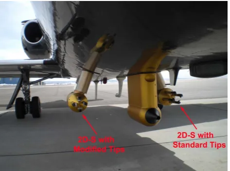
Figure 3. Photograph showing the SPEC Learjet used in the SPARTICUS project with two 2D-S probes, one with tips modified to reduce shattering, and the other with standard tips.
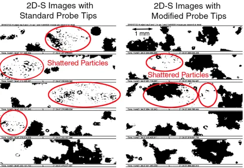
The images in Fig. 5 suggest, and the size distributions in Fig. 6 support the premise that the modified probe tips significantly reduce, but do not eliminate shattering. During the penetration of precipitating dendrites, post processing of the 2D-S probe with standard tips identified 153 out of 507 (30%) of the images > 1 mm as shattered images. In comparison, the modified probe tips eliminated more than half this amount, with 54 out of 450 (12%) of the images > 1 mm being identified as shattered images.
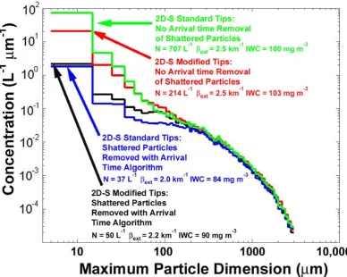
Figure 6 shows that the size distribution with the unmodified probe tips and without application of the arrival time removal algorithm (green trace) contains the most particles with sizes < 200 m. The size distribution with modified probe tips and without application of the arrival time removal algorithm (red trace) contains the second most particles with sizes < 200 m, which also shows that the probe with modified probe tips is effective in reducing shattering. However, the two size distributions that have been processed using the arrival time algorithm to remove shattered particles contain far fewer particles < 200 m than either
paper, the two (H and V) channels of each probe were averaged, and only regions where the two channels were in good agreement were used, avoiding any regions where obvious instrumentation effects adversely influenced the measurements.
Fig. 3. Photograph showing the SPEC Learjet used in the SPARTI-CUS project with two 2D-S probes, one with tips modified to reduce shattering, and the other with standard tips.
and fabricated based on information that Korolev delivered in person to SPEC engineers. Appendix C shows photographs and drawings of 2D-S probe tips that are germane to this pa-per. As shown in Fig. 3, the “standard” and “modified” 2D-S probes were about 1.5 m apart and were identical except for the probe tips. However, it is always important to keep in mind that even though two particle imaging probes are constructed to be identical, their comparative performance is rarely identical (e.g., Gayet et al., 1993).
On 23 July 2010 the Learjet penetrated a cloud region with only small cloud drops, where no shattering is expected, and a region of precipitation with large ice aggregates, where shattering is expected. Figure 4 shows average 2D-S drop size distributions in the region with only small cloud drops, with and without application of the shattering algorithm, for both 2D-S probes shown in Fig. 3. There is reasonably good agreement between the two probes in the cloud with only small drops where no shattering is expected, and applica-tion of the shattering algorithm had a negligible effect on the drop size distributions. This demonstrates that on this mission both probes recorded similar concentrations of small particles when there were no shattering effects. Later in the mission, the Learjet penetrated near the base of a thunder-storm anvil that contained a wide range of ice particle sizes, extending out to a few millimeters. This 3-min segment was selected because it was the only period with millimeter-size precipitating ice that the Learjet encountered on this mission. Figure 5 shows examples of typical images from both probes, i.e., with unmodified and with modified probe tips. Figure 6 shows a comparison of particle size distributions from the two 2D-S probes, with and without modified tips; and with and without application of the arrival time shattering removal algorithm. Figure 6 shows that all of the size distributions
of the other size distributions, regardless whether the probe has modified tips, or not. Thus, in this case, the arrival time algorithm is more effective than the modified probe tips in reducing the effects of shattering on these 2D-S probes.
The average bulk parameters, total number concentration (N), extinction coefficient (ext)
and ice water content (IWC) are also shown in Fig. 6. In this example, without application of
the arrival time algorithm the modified tips make a significant difference in N (707 L-1 vs 214 L-1). Application of the arrival time algorithm reduces N from 707 L-1 to 37 L-1 with the standard tips and from 214 L-1 to 50 L-1 with the modified tips. Thus, the modified tips reduce N by 493 L-1 and application of the arrival time algorithm reduces N by only an
additional 177 L-1. On the other hand, without application of the arrival time algorithm the
modified tips make no difference in ext and only 3 mg difference in IWC. When the arrival
algorithm is used in the computation of ext and IWC, the differences are much larger.
Application of the arrival time algorithm reduces ext from 2.5 km-1 to 2.0 km-1 with the
standard tips, and from 2.5 km-1 to 2.2 km-1 with the modified tips. The arrival time
algorithm reduces IWC from 100 mg m-3 to 84 mg m-3 with the standard tips, and from 103
mg m-3 to 90 mg m-3 with the modified tips. Thus, in this example application of the arrival
time algorithm makes a much more significant impact on the second and third moments of the size distribution than does the modified tips.
Figure 4. 2D-S size distributions from Learjet penetration (205408 205421 UTC on 23 July
2010) of a small cumulus cloud containing only water drops. The light green trace is from the probe with standard tips and includes shattered particles. A dark green trace is from the
Fig. 4. 2D-S size distributions from Learjet penetration (20:54:08 to 20:54:21 UTC, 23 July 2010) of a small cumulus cloud contain-ing only water drops. The light green trace is from the probe with standard tips and includes shattered particles. A dark green trace is from the probe with standard tips after applying the shattering algo-rithm, but is not visible behind the light green trace. The red trace is from the probe with modified tips and includes shattered particles. A blue trace from the probe with modified tips after applying the shattering algorithm is barely visible near the red trace.
tend to converge at particle sizes larger than about 200 µm, which suggests that (in this case) the erroneous effects of shattering are less apparent in the larger portion of the size distribution.3
The images in Fig. 5 suggest, and the size distributions in Fig. 6 support the premise that the modified probe tips significantly reduce, but do not eliminate shattering. During the penetration of precipitating dendrites, post processing of the 2D-S probe with standard tips identified 153 out of 507 (30 %) of the images>1 mm as shattered images. In com-parison, the modified probe tips eliminated more than half this amount, with 54 out of 450 (12 %) of the images>1 mm being identified as shattered images.
3Note that each 2D-S probe used in this study actually contains
1366 R. P. Lawson: Effects of ice particles shattering on the 2D-S probe
probe with standard tips after applying the shattering algorithm, but is not visible behind the
light green trace. The red trace is from the probe with modified tips and includes shattered
particles. A blue trace is from the probe with modified tips after applying the shattering
algorithm is barely visible near the red trace.
Figure 5.
Examples of 2D-S images from two 2D-S probes flown side-by-side on the SPEC
Learjet (
Fig. 3
) during the SPARTICUS project, one probe had standard 2D-S probe tips
(left) and (right) the other with tips modified to reduce the effects of shattering.
Fig. 5. Examples of 2D-S images from two 2D-S probes flown side-by-side on the SPEC Learjet (Fig. 3) during the SPARTICUS project, one probe had standard 2D-S probe tips (left) and (right) the other with tips modified to reduce the effects of shattering.
Figure 6 shows that the size distribution with the unmod-ified probe tips and without application of the arrival time removal algorithm (green trace) contains the most particles with sizes <200 µm. The size distribution with modified probe tips and without application of the arrival time removal algorithm (red trace) contains the second most particles with sizes<200 µm, which also shows that the probe with modi-fied probe tips is effective in reducing shattering. However, the two size distributions that have been processed using the arrival time algorithm to remove shattered particles contain far fewer particles<200 µm than either of the other size dis-tributions, regardless whether the probe has modified tips, or not. Thus, in this case, the arrival time algorithm is more ef-fective than the modified probe tips in reducing the effects of shattering on these 2D-S probes.
The average bulk parameters, total number concentration (N ), extinction coefficient (βext)and ice water content (IWC)
are also shown in Fig. 6. In this example, without application of the arrival time algorithm the modified tips make a signifi-cant difference inN(707 l−1vs. 214 l−1). Application of the arrival time algorithm reducesN from 707 l−1to 37 l−1with
the standard tips and from 214 l−1 to 50 l−1with the modi-fied tips. Thus, the modimodi-fied tips reduceN by 493 l−1 and application of the arrival time algorithm reducesN by only an additional 177 l−1. On the other hand, without application
of the arrival time algorithm the modified tips make no dif-ference inβext and only 3 mg difference in IWC. When the
arrival algorithm is used in the computation ofβextand IWC,
the differences are much larger. Application of the arrival time algorithm reducesβextfrom 2.5 km−1to 2.0 km−1with
the standard tips, and from 2.5 km−1 to 2.2 km−1 with the modified tips. The arrival time algorithm reduces IWC from 100 mg m−3to 84 mg m−3with the standard tips, and from 103 mg m−3to 90 mg m−3with the modified tips. Thus, in this example application of the arrival time algorithm makes a much more significant impact on the second and third mo-ments of the size distribution than does the modified tips.
R. P. Lawson: Effects of ice particles shattering on the 2D-S probe 1367
Figure 6. Average particle size distributions derived from 2D-S measurements collected in
large ice aggregates from 213418 - 213716 UTC on 23 July 2010. Data are from two 2D-S probes installed side-by-side on the SPEC Learjet (Figs. 3 - 5). One probe had standard probe
tips and the other probe was equipped with probe tips modified to reduce shattering. Size distributions are shown with and without the effects of an arrival time algorithm to remove shattering. Total particle concentration (N), extinction coefficient (ext) and ice water content (IWC) were derived from each average size distribution.
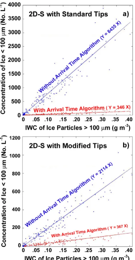
Another method for examining the effects of shattering is to generate a scatter plot of the concentration of small (shattered) particles versus the mass of large (shattering) particles (Jensen et al. 2009). In this way, it is possible to see if the concentration of smaller particles that may (or may not) have been generated from shattering, are correlated with increasing mass of large particles, which are responsible for generating shattered particles. Figure 7
shows 1-Hz scatter plots of 2D-S data with standard tips and with modified tips from the 213418 – 213716 UTC 23 July 2010 SPARTICUS anvil penetration discussed above. As seen in Fig. 7a, the scatter plot with the standard tips shows a very strong correlation
between the concentration of small particles and increasing ice water content without application of the arrival time algorithm. After application of the arrival time algorithm there is still a correlation, but the magnitude of the trend is considerably less. Figure 7b shows
that the modified tips reduces the number of small (shattered) particles, but the correlation between the concentration of small particles and increasing ice water content is still strong.
Fig. 6. Average particle size distributions derived from 2D-S measurements collected in large ice aggregates from 21:34:18–21:37:16 UTC, 23 July 2010. Data are from two 2D-S probes installed side-by-side on the SPEC Learjet (Figs. 3–5). One probe had standard probe tips and the other probe was equipped with probe tips modified to reduce shattering. Size distributions are shown with and without the effects of an arrival time algorithm to remove shattering. Total particle concentration (N), extinction coefficient (βext)and ice water content (IWC) were
derived from each average size distribution.
have been generated from shattering, are correlated with in-creasing mass of large particles, which are responsible for generating shattered particles. Figure 7 shows 1-Hz scat-ter plots of 2D-S data with standard tips and with modified tips from the 21:34:18–21:37:16 UTC, 23 July 2010 SPAR-TICUS anvil penetration discussed above. As seen in Fig. 7a, the scatter plot with the standard tips shows a very strong correlation between the concentration of small particles and increasing ice water content without application of the ar-rival time algorithm. After application of the arar-rival time algorithm there is still a correlation, but the magnitude of the trend is considerably less. Figure 7b shows that the modified tips reduces the number of small (shattered) particles, but the correlation between the concentration of small particles and increasing ice water content is still strong. Application of the arrival time algorithm reduces the shattering trends in Fig. 7a and b to about the same magnitude, regardless whether the probe has standard or modified tips. The data in Fig. 7 sug-gests that, in this case, the arrival time algorithm produces approximately the same result, regardless of whether the 2D-S probe has standard or modified tips. The data also
sug-gest that using the 2D-S probe with modified tips alone is not sufficient to reduce shattering to the level achieved after the arrival time algorithm is applied.
The scatter plots in Fig. 7 can also be interpreted to pro-vide an estimate of the effectiveness of removing small ice particles due to shattering, or alternatively, an estimate of the maximum number of natural small ice particles. For exam-ple, the data in Fig. 7 show that for this particular case, for the unmodified tips, approximately 8500 l−1of (spurious) small ice particles are produced for each g m−3of large ice. Sim-ilarly, measurements from the probe with the modified tips show that about 2000 l−1small ice particles are produced for
each g m−3of large ice. Since both probes yield about the
1368 R. P. Lawson: Effects of ice particles shattering on the 2D-S probe
Figure 7. Scatter plots of the concentration of ice particles < 100 m versus ice water
content. Data collected in large ice aggregates with two 2D-S probes installed side-by-side on the SPEC Learjet (Figs. 3 - 6). One probe (a) had standard probe tips and the other probe
(b) was equipped with probe tips modified to reduce shattering. Effect of the arrival time algorithm to remove shattering is shown on each plot.
Fig. 7. Scatter plots of the concentration versus ice water content of ice particles<100 µm. Data collected in large ice aggregates with two 2D-S probes installed side-by-side on the SPEC Learjet (Figs. 3–6). One probe (a) had standard probe tips and the other probe (b) was equipped with probe tips modified to reduce shat-tering. Effect of the arrival time algorithm to remove shattering is shown on each plot.
shattering, i.e, in this case∼350 l−1of small ice particles per
g m−3 of large ice remain after shattering prevention with modified tips and removal with the arrival time algorithm. Since it is not possible to know the actual concentration of small ice particles, in this case: (1) 350 l−1per g m−3is an estimate of the upper bound of the possible remaining effects of shattering, or (2) an upper bound of the natural ice con-centration in the cloud.
The measurements shown in Figs. 6 and 7 suggest that the modified tips reduce the number of small (shattered) par-ticles, but not as effectively as the arrival time algorithm. Also, there is still a trend for increasing small particles with increasing ice water content, even with modified tips and ap-plication of the arrival time algorithm. This can be explained either by a process that is actually generating small particles when there are more large ice particles (e.g., particle-particle collisions), or that not all of the shattered particles are being removed by the modified tips and arrival time algorithm. We would like to point out a scenario where a shattered particle can be counted as a natural ice particle. If only one shattered small particle passes through the sample volume (i.e., the re-mainder of the shattered small particles are out of the depth of field), the one small particle in the depth of field will be not be rejected by the arrival time algorithm and will be counted as a natural ice particle (Korolev et al., 2010a). Since the depth of field of imaging probes is very small for small parti-cles, the effective particle concentration is increased dramat-ically. The probability of this occurring is unknown at this time and would require a dedicated investigation, perhaps requiring high-speed video of shattered particles in various airborne flight and cloud conditions. However, the method-ology presented here (i.e., Fig. 7 and associated discussion) is a method for estimating the maximum contribution from shattering.
After examining the data in Fig. 7, it is tempting here to state that shattering may have artificially increased the con-centration of small particles by an order of magnitude. How-ever, it is important to keep in mind that the contribution from shattering is relative to the natural concentration of small par-ticles. If the contribution from shattering of very large parti-cles in the example in Fig. 7 was hypothetically added to the concentration of natural small particles at the top of the cirrus cloud example in Fig. 2, then the contribution from shattering would add<10 % to the total particle concentration. For this reason, we recommend reporting quantified additive effects and to avoid reporting multiplicative values.
3.2 AIIE field campaign
R. P. Lawson: Effects of ice particles shattering on the 2D-S probe 1369
Fig. 8. Particle size distributions from 14:09:00–14:21:00 UTC, 8 April 2009, collected during the AIIE field project. Data are repro-duced from Korolev et al. (2010b) with the addition of 2D-S data for the same time period. “stand.” Means standard probe tips; “modif.” means modified probe tips, “corr.” means data have been adjusted using an arrival time algorithm and “no corr.” means that no arrival time algorithm has been applied.
arrival time algorithm (indicated by “corr.” in the figure)4. The CIP data in Fig. 8b shows the same trend as the 2D-C in Fig. 8a. In Fig. 8a and b, 2D-S data without (“no corr.”) and with (“corr.”) arrival time corrections are shown with mod-ified probe tips. A comparison of all data in Fig. 8 suggest that the 2D-S probe with application of arrival time correc-tion removes the most small (shattered) particles. The 2D-C probe with arrival time correction is closest to the 2D-S PSD, with the CIP probe showing the most deviation from the 2D-S results.
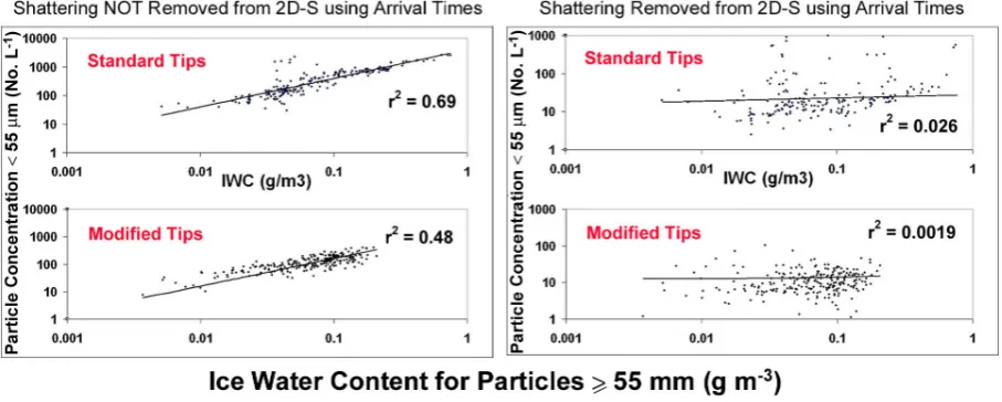
Figure 9 shows 2D-S measurements from data collected during the AIIE field program on two different flights in sim-ilar cloud conditions; one flight when the probe was flown
4The particle arrival time algorithm applied to the AIIE data
was developed and applied by Alexei Korolev.
without modified probe tips, and the second flight with mod-ified tips. Each data point in Fig. 9 represents a 15 to 30 s average calculated in the following way. One-hertz data 2D-S are screened for periods when the large (>55 µm) particle concentration exceeds 1 m−3for a minimum of 15 s. During this period the 1-Hz median volume diameter must remain between 0.8 and 1.2 of its mean and the large particle con-centration must remain between 0.4 and 2.0 of its mean. If an accepted time period exceeds 30 s the first 15 s are cut off as a separate period and the algorithm continues. So all ac-cepted periods are between 15 and 30 s in duration. 2D-S data from the flights with and without the modified tips were processed with and without application of the arrival time al-gorithm, producing the four scatter plots seen in Fig. 9. The data in Fig. 9 show that without applying the arrival time al-gorithm, the concentration of small (<55 µm) ice particles is about 6000 l−1per g m−3with the unmodified tips,
com-pared with about 1000 l−1per g m−3with the modified tips.
However, there is still a strong correlation between increas-ing concentration of small particles and ice water content, until the application of the arrival time algorithm. Once the arrival time algorithm is applied the average concentration of small ice particles is about 20 l−1 per g m−3 with both the unmodified and modified tips, and there is no correlation be-tween increasing small ice particles and ice water content.
The data in Fig. 9 suggest that, for the 2D-S probe in these cloud conditions, the modified tips reduce, but do not elim-inate the trend of increasing small particles with increasing ice water content. On the other hand, the data in Fig. 9 do show that, in this case, the arrival time algorithm eliminates the correlation between large and small (shattered) particles. It should be pointed out, however, that because there is no way of knowing the actual concentration of small particles (i.e., there could be none), this does not imply that the ar-rival time algorithm eliminates all of the shattered particles. As in Fig. 7, though, an estimate of the upper bound on the amount of shattered ice particles and natural ice particles can be derived from these scatter plots. The results shown in Figs. 7 and 9 are only two examples, and shattering is likely to depend on many factors, including ice crystal size, type, airspeed, angle of attack and temperature, to mention some of the more important factors. For example, the data in Fig. 7 still show a (weak) correlation between large and small par-ticles in the large particle region of an anvil cloud, even with modified tips and application of the arrival time algorithm. 3.3 ISDAC field campaign
1370 R. P. Lawson: Effects of ice particles shattering on the 2D-S probe
Fig. 9. Scatter plots of the concentration of ice particles (<55 µm) versus ice water content=>55 µm. Data were collected during the AIIE field project with a 2D-S probe installed on the NRC Convair 580. Data were collected with standard tips from 17:54:53–20:16:44 UTC, 1 April 2009. Data were collected with modified tips from 14:32:32–16:24:37 UTC, 4 April 2009. The 2D-S probe was flown with standard tips on one flight (top two panels), then with modified tips in similar conditions on a second flight (bottom two panels). Effect of the arrival time algorithm to remove shattering is shown on plots on the right side.
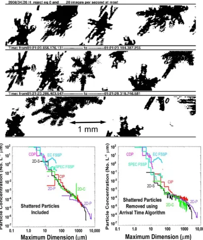
stratus cloud investigated from 01:20:00 to 01:26:40 UTC, 26 April 2008. The instrument acronyms shown on the fig-ures and their affiliations are listed in the figure caption. Fig-ure 11 shows typical particle images and size distributions from the same instruments flown in the mixed-phase region 300 m above the base of the same Arctic stratus cloud from 02:48:40 to 02:48:53 UTC. Only the 2D-C had probe tips with an aggressive design to reduce shattering. However, the 2D-S probe did have tips that were designed to reduce shat-tering, based on understanding of ice particle shattering at that time.
The lower left sides of Figs. 10 and 11 show size distri-butions without removing shattered particles, while the right sides show the same time periods using an arrival time algo-rithm to remove shattered (i.e., closely spaced) particles on the SPEC 2D-S and fast FSSP, the EC 2D-C and the DMT CIP.5The size distributions without application of the arrival time algorithm are all in reasonably good agreement, both below cloud base in precipitating dendrites (where small par-ticles are not thought to be abundant), and in the mixed-phase region where the CDP and FSSP probes show about 80 cm−3.
In the precipitating dendrite size distributions (Fig. 10), the SPEC fast FSSP and 2D-S probes show a significant reduc-tion in the concentrareduc-tion of small particles with the arrival time algorithm applied. The particle concentration in the size range from 5 to 300 µm is reduced from about 20 to 2 l−1. The 2D-C, which has a 25- µm pixel size, also shows a re-duction in particle concentration of about 3 to 0.3 l−1in the 25 to 300 µm size range. On the other hand, there is very
lit-52D-C and CIP arrival time algorithm developed and applied by
Greg McFarquhar’s group at the University of Illinois.
tle change in the CIP size distribution and the small particle concentration actually increases in the smallest bins (due to re-sizing of some of the larger donut-shaped particles). In this case the application of an arrival time algorithm has a result similar to the AIIE results shown in Fig. 8, where both the 2D-S and 2D-C size distributions show significant reduc-tions in small particles, whereas the CIP shows much less of an effect.
In the mixed-phase region of the same cloud (Fig. 11), the natural small particle (i.e., cloud drop) concentration is about 80 cm−3, which is much higher than below cloud base. Even though the concentration of large particles in the mixed-phase is about the same as in the precipitation below cloud base, the total particle concentration is not significantly affected when the arrival time algorithm is applied. The most significant difference when the arrival time algorithm is applied is seen in the region from about 50 to 150 µm, but the percentage change is still quite small. When shat-tered particles are removed particle concentration in the 50 to 150 µm size range changes from 1.4 to 0.4 l−1, extinction coefficient goes from 0.08 to 0.05 km−1and ice water con-tent changes from 7 to 5 mg m−3. The percentage change in small (cloud drop) particles when shattered particles are removed is negligible. Particle concentration changes from 66 304 to 66 295 l−1, extinction coefficient goes from 10.78
R. P. Lawson: Effects of ice particles shattering on the 2D-S probe 1371
Figure 10
shows typical particle images and size distributions from several particle probes
that were flown together below the base of a precipitating Arctic stratus cloud investigated
from 01:20:00 to 01:26:40 UTC on 26 April 2008. The instrument acronyms shown on the
figures and their affiliations are listed in the figure caption.
Figure 11
shows typical particle
images and size distributions from the same instruments flown in the mixed-phase region 300
m above the base of the same Arctic stratus cloud from 02:48:40 to 02:48:53 UTC. Only the
2D-C had probe tips with an aggressive design to reduce shattering. However, the 2D-S
probe did have tips that were designed to reduce shattering, based on understanding of ice
particle shattering at that time.
Figure 10. (
top
)
2D-S Images and (bottom) particle size distributions from several cloud
particle probes flown on the Canadian Convair 580 in precipitating dendrites below cloud
Fig. 10. (top) 2D-S Images and (bottom) particle size distributions from several cloud particle probes flown on the Canadian Convair 580 in precipitating dendrites below cloud base during ISDAC from 01:20:00 to 01:26:40 UTC, 26 April 2008. Left panel shows measurements with shattered particles included and right panel with shattered particles removed using arrival time algorithm. EC FSSP = Environment Canada FSSP. CDP = DMT CDP. SPEC FSSP = SPEC Fast FSSP. CIP = DMT CIP. 2DC = EC 2DC. 2DP = EC.
makes a significant contribution to total particle concentra-tion, whereas this is not the case when the natural ice con-centration is high.
3.4 MACPEX field campaign
1372 R. P. Lawson: Effects of ice particles shattering on the 2D-S probe
base during ISDAC from 01:20:00 to 01:26:40 UTC on 26 April 2008. Left panel shows
measurements with shattered particles included and right panel with shattered particles
removed using arrival time algorithm. EC FSSP = Environment Canada FSSP. CDP = DMT
CDP. SPEC FSSP = SPEC Fast FSSP. CIP =
DMT CIP. 2DC = EC 2DC. 2DP = EC
Figure 11.
As in
Fig. 10
, except data were collected in the mixed-phase region of the same
Arctic cloud from 02:48:40 to 02:48:53 UTC on 26 April 2008.
The lower left sides of
Figs. 10
and
11
show size distributions without removing
shattered particles, while the right sides show the same time periods using an arrival time
algorithm to remove shattered (i.e., closely spaced) particles on the SPEC 2D-S and fast
Fig. 11. As in Fig. 10, except data were collected in the mixed-phase region of the same Arctic cloud from 02:48:40 to 02:48:53 UTC, 26 April 2008.
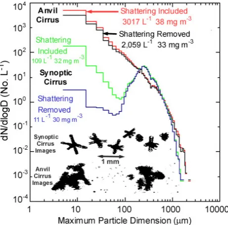
physical credibility to the very large differences in 2D-S par-ticle concentrations observed in the two regimes. The high particle concentration in the anvil cirrus is the result of ho-mogeneous freezing of drops in convective updrafts and sub-sequent outflow in the anvil. Fridlind et al. (2004) show that model simulations produce in excess of 10 cm−3of ice par-ticles in the convective outflow regions of anvils. On the other hand, Comstock et al. (2008) show numerical simu-lations of synoptic cirrus with typical concentrations of 1
to 100 l−1. Consistent with simple physical arguments and numerical simulations, Fig. 12 shows relatively low (11 l−1)
R. P. Lawson: Effects of ice particles shattering on the 2D-S probe 1373
relatively low (11 L-1) concentrations of small particles in cirrus that was generated
synoptically, and much higher (2,059 L-1) concentrations of small particles in anvil cirrus,
located several km downwind of convection. Note that unlike Figs. 1 and 2, the ordinate in Fig. 3 is dN/dlogD, which tends to emphasize the reduction of small particles in the plot.
Figure 12. Particle size distributions as a function of concentration from 2D-S probe measurements in anvil and synoptic cirrus sampled on 14 April 2011 from 183600 – 185100 UTC (synoptic cirrus), and 11 April 2011 from 173750 – 184610 UTC (anvil cirrus) by the NASA WB-57 during the MACPEX field campaign. Example 2D-S images from each time period are shown below the size distributions.
The data in Fig. 12 are also a good example of how quoting multiplicative shattering factors can be very misleading. The shattering algorithm reduces the total number concentration in the synoptic cirrus by an order of magnitude (i.e., from 109 L-1 to 11 L-1),
while the anvil particle concentration is only reduced by 32% (i.e., from 3,017 L-1 to 2,059 L -Fig. 12. Particle size distributions as a function of concentration from 2D-S probe measurements in anvil and synoptic cirrus sam-pled on 14 April 2011 from 18:36:00–18:51:00 UTC (synoptic cir-rus), and 11 April 2011 from 17:37:50–18:46:10 UTC (anvil cirrus) by the NASA WB-57 during the MACPEX field campaign. Exam-ple 2D-S images from each time period are shown below the size distributions.
The data in Fig. 12 are also a good example of how quot-ing multiplicative shatterquot-ing factors can be very misleadquot-ing. The shattering algorithm reduces the total number concen-tration in the synoptic cirrus by an order of magnitude (i.e., from 109 l−1to 11 l−1), while the anvil particle concentration is only reduced by 32 % (i.e., from 3017 l−1 to 2059 l−1). However, the total number concentration of anvil particles removed by the algorithm (958 l−1)is an order of magnitude greater than the synoptic cirrus value (98 l−1). Thus, report-ing only the multiplicative factor in the synoptic cirrus case can lead readers to assume that the order of magnitude con-centration enhancement due to shattering could also apply to other cases, leading to erroneous conclusions.
The data shown in Fig. 12 also beg a question: why, with roughly the same total mass in each size distribution, does shattering in the anvil regime appear to produce 10 times the concentration of shattered particles? Fig. 13, which shows the anvil and synoptic cirrus size distributions as a function of mass, provides some insight. While the total mass in parti-cles>∼100 µm is roughly the same in both size distributions, there is significantly more mass in sizes>1 mm in the anvil compared to the synoptic cirrus. Also, as shown in several previous studies, and the 2D-S images in Fig. 12, the mass distribution in synoptic cirrus is dominated by bullet rosette shapes, while anvils are typically composed of plates, aggre-gates of plates and columns (Connolly et al., 2005; Lawson
Figure 13. As in Fig. 12 except the size distributions are shown as a function of particle mass.
Two 2D-S probes, one with and one without modified probe tips, were flown side-by-side on the SPEC Learjet in the SPARTICUS field project. The modified probe tips were designed with the assistance of Dr. Korolev, and are based on theory and knowledge learned from the icing tunnel videography. Analysis of data collected in large aggregates shows that the modified 2D-S probe tips substantially reduce the number of small (shattered) particles; however, post-processing with the arrival time algorithm is more effective, whether applied to the probe with modified or unmodified tips. This is contrary to the results for the 2D-C and CIP presented by Korolev et al. (2010b).
Fig. 13. As in Fig. 12 except the size distributions are shown as a function of particle mass.
et al., 2006b, 2010; Protat et al., 2011). In addition, Connolly et al. (2005) show that mid-latitude anvils often contain ag-gregated chains of small plates that could easily break apart when shattered. The observations in Figs. 12 and 13 fur-ther emphasize the complexity of the shattering issue and the need for more detailed study, including systematic studies of the shattering characteristics of particles with different sizes and shapes.
4 Summary and discussion
The effects of ice particles shattering on the tips of the 2D-S optical array probe, referred to in this paper as “shattering”, are investigated. While shattering has been known for over 35 yr, under certain cloud conditions the magnitude of the contribution of shattered particles can be significant. NASA GRC supplied high-speed video photography in the Cox & Company icing tunnel of ice particles shattering on the tips of cloud particle probes. Korolev et al. (2010a) show that ice particles a few hundreds of microns in size shatter into hun-dreds of small ice particles with sizes that range from about 10 to 100 µm. As suggested from the comparison of 2D-S particle images in Fig. 5 and size distributions in Figs. 6, 10, 12 and 13, the large majority of these particles are in the size range from 10 to 50 µm (or perhaps even smaller).
1374 R. P. Lawson: Effects of ice particles shattering on the 2D-S probe particles are much more closely spaced than natural ice
dis-tributions.
Korolev et al. (2010b) report results from analysis of 2D-C and 2D-CIP data collected from a field campaign (AIIE) that was designed to evaluate the effects of shattering on cloud particle probes. 2D-C and CIP probes, each with standard tips and tips modified by Korolev6were flown side-by-side on the Canadian CV-580. The results show that the modified probe tips were more effective reducing shatterers than post-processing with an arrival time algorithm.
Two 2D-S probes, one with and one without modified probe tips, were flown side-by-side on the SPEC Lear-jet in the SPARTICUS field project. The modified probe tips were designed with the assistance of Korolev, and are based on theory and knowledge learned from the icing tun-nel videography. Analysis of data collected in large aggre-gates shows that the modified 2D-S probe tips substantially reduce the number of small (shattered) particles; however, post-processing with the arrival time algorithm is more effec-tive, whether applied to the probe with modified or unmodi-fied tips. This is a different result than Korolev et al. (2010b) obtained for the 2D-C and CIP probes.
Korolev et al. (2010a) discuss a possible explanation for the apparent ineffectiveness of the arrival time approach when applied to the 2D-C and CIP probes. Due to the (50 µm to 100 µm) effective size resolution of the CIP and 2D-C, the imagery may miss many of the small shattered particles, producing large gaps that defeat the arrival time algorithm, and/or groups of small particles that are blurred together and appear as one larger particle. The explanation offered by Ko-rolev et al. (2010a) is that it may appear that one (shattered) particle passes through the sample volume and is counted as a real particle. Because depth of field and thus sample volume are inversely proportional to the square of particle size, the one event generates a much higher concentration than does a large particle. The faster time response and greater effec-tive size resolution of the 2D-S probe may enable it to more accurately reproduce particle spacing in a burst of shattered particles, which may make its particle arrival time algorithm more effective.
Results from SPARTICUS, ISDAC, AIIE and MACPEX show that post-processing 2D-S data with the arrival time al-gorithm (see Appendices A and B) is very effective in mini-mizing the effects of shattered ice particles. For the first time, measurements from major field programs (e.g., SPARTI-CUS, TC4, MACPEX) show vertical profiles of ice particle concentration in deep ice clouds (anvils and deep cirrus) that are consistent with physical arguments and numerical mod-els. That is, relatively high concentrations of small ice near cloud top with decreasing concentration of small ice toward cloud base. Data from previous field campaigns (e.g., Law-son et al., 2006b) show increasing concentrations of small ice toward cloud base due to shattering on the older probes. A
6See footnote # 2.
comparison of 2D-S particle concentrations from MACPEX in synoptically generated cirrus and a convectively generated anvil also more closely represent results from physical argu-ments and numerical simulations.
The effect of shattering on the second (extinction) and third (ice water content) moments of a cloud particle size distribution can be either minimal, or significant, depending on the instrument, cloud conditions and application of the measurements. The worse situation appears to be when scat-tering probes, such as the FSSP and the cloud and aerosol spectrometer (CAS), with tubular inlets, are used to mea-sure ice particles in environments with high mass concentra-tions of large ice. Jensen et al. (2009) suggests that measure-ments under these conditions significantly skew the second moment of the size distribution, which generates the poten-tial for misleading radiative computations. Ice water content is not as strongly affected as extinction, but significant errors can occur, such as suggested when an FSSP is used to mea-sure small ice particles near the bases of deep cirrus clouds (Lawson et al., 2006b), or when a CAS is used to measure small particle concentration in thunderstorm anvils (Garrett et al., 2005; Fridlind et al., 2004).
All of the shattering results presented here are based on analyses of a few cases, using only three research aircraft, and in a limited number of cloud conditions and flight config-urations. Results of the effects of shattering from the SPAR-TICUS, AIIE, ISDAC and MACPEX projects cannot be con-sidered comprehensive or statistical. A statistical analysis was not possible with the available dataset and was not the focus of this paper. The takeaway message is that the lim-ited dataset indicates that a post-processing algorithm based mainly on particle arrival times is more effective than mod-ified 2D-S probe tips in reducing the effects of shattering. This result differs from analysis of a shattering analysis re-ported by Korolev et al. (2011b), who found that modified probe tips were more effective than a particle arrival time al-gorithm in reducing shattering on the CIP and 2D-S probes.
R. P. Lawson: Effects of ice particles shattering on the 2D-S probe 1375 5 Major conclusions
– The effects of ice particles shattering on the tips of 2D-S probes are reduced by modified tips based on the design of Korolev7, and by post-processing based on an inter-arrival time algorithm (Appendices A and B). However, the inter-arrival time algorithm appears to be more ef-fective than the modified tips with applied to 2D-S data, although use of both techniques is synergistic and rec-ommended. This is a different result than obtained by Korolev et al. (2010b) from the AIEE field campaign, where it is reported that modified tips on CIP and 2D-C probes are more effective than an arrival time algorithm in reducing the effects of shattering.
– When compared to measurements from previous field campaigns that used older cloud particle probes, 2D-S data (with shattering removed) collected in recent (i.e., TC4, SPARTICUS, MACPEX) field campaigns show results that are consistent with physical arguments and numerical simulations. For example, ice particle con-centrations in synoptic cirrus are two orders of magni-tude less than anvil cirrus, even though total mass con-centrations are similar in the regions selected for this analysis. Also, the vertical distribution of small ice par-ticles in deep ice clouds decreases with distance from cloud top while the total mass of ice increases.
– A rigorous quantification of the effects of ice particles shattering on the inlets and tips of optical cloud particle probes is a complicated undertaking, because shattering is contingent on many factors that are a function of the probe, aircraft and environmental properties. However, Figs. 7 and 9, and other scatter plots of this type found in the literature, provide a methodology that forms a crude quantification of the upper bound of the effects of shattering. A comprehensive experiment with per-haps high-speed, in-flight video and extensive measure-ments in varying cloud regimes and aircraft configura-tions could shed more light on the physical processes involved in shattering, and also form the basis for statis-tical analysis.
Appendix A
Software processing of 2D-S Data
Processing of 2D-S image data is a complex process that has evolved based on both theoretical and empirical approaches. Image analysis and derived products include the convolution of multiple algorithmic processes. The convolution of algo-rithms includes software techniques that make adjustments to particle concentration and size that are used in both the
7See footnote #2.
basic processing and removal of shattered particles. Thus, there is crossover of some techniques from one process to another (and consequently from Appendix A to Appendix B, and vice versa). The processing can loosely be divided into three broad steps:
– Various methods to determine “characteristic” lengths,
Li, and areas,Ai, of an image.
– Removal of what are called here “spurious” events (also referred to as artifact rejection), which can include elec-tronic noise, optical contamination, particle shattering and splashing effects.
– Various methods, Mi, of estimating the bulk physical
parameters; concentration, extinction, and mass as func-tions of size. These include correction for diffraction effects based on the Korolev (2007) methodology and adjustments to sample volume as a function of particle size.
These algorithmic processes require the introduction of various parameters that are defined throughout this Appendix and in Appendix B.
There are several different ways thatLi can be measured.
Figure A1 is a schematic depicting four measures of image length used in 2D-S analysis.L1is the number of slices
(pix-els in the direction of travel) for which a particle event lasted.
L2is the number of shaded photodiodes (pixels in the
direc-tion along the array) for the slice for which the same quantity is maximized. L4is the number of diodes between, and
in-cluding the shaded end diodes, for the slice that maximizes the same quantity.L5is the distance between (and including)
the shaded end diodes considering all of the slices together.8 The appropriate selection ofLidepends on the size and type
of particles that are being imaged. For example, if particle sizes exceed the (1.28 mm) viewing area of the 2D-S, use of L2 would limit the maximum particle size to 1.28 mm,
whereas use of L1 would provide a one-dimensional
mea-surement of particles of any length, providing any part of the particle remained in the viewing area.
Several other size parameters are used in processing an image.L7is the diffraction-corrected length for out-of-focus
(“donut”) images based on Korolev (2007). As is the
num-ber of occulted pixels for the entire image (summed over all slices).Atis the total number of pixels (occulted or not)
con-tained within an image, which was developed by Korolev and is used in the Korolev (2007) diffraction-correction method.
The accepted particles are binned according to size. The size bin’s edges are: [5, 15, 25, 35, 45, 55, 65, 75, 85, 95, 105, 115, 125, 135, 145, 155, 165, 175, 185, 195, 205, 225, 245,
8Note that the numbering of the “L” lengths is not
1376 R. P. Lawson: Effects of ice particles shattering on the 2D-S probe
Figure A.1
. Two example particle images designed to demonstrate
the four measures of image size described in this Appendix.
The accepted particles are binned according to size. The size bin’s edges are: [5, 15, 25, 35,
45, 55, 65, 75, 85, 95, 105, 115, 125, 135, 145, 155, 165, 175, 185, 195, 205, 225, 245, 265,
285, 305, 325, 345, 365, 385, 405, 425, 465, 485, 505, 555, 605, 655, 705, 755, 805, 855,
905, 955, 1005, 1105, 1205, 1305, 1405, 1505, 1605, 1705, 1805, 1905, 2005, 2205, 2405,
2605, 2805, 3005, 3205, 3405, 3605, 3805, 4005, 4205, 4405, 4605, 4805, 5005, 6005, 6505,
7005, 7505, 8005, 8505, 9005, 9505, 10005, 10505, 11005, ∞].
Next we present general equations for calculating bin particle concentration, bin particle
area assuming spheres, bin particle area not assuming spheres, bin liquid water content
(LWC) and bin ice water content (IWC). The adjustment factor
SV
adjand sample volume
(
SV
) are defined in specific terms later in Appendix B and below, respectively.
The general equation for a bin’s concentration is:
)
(
#
BW
SV
counts
where #
countsis the number of particles counted in that size bin,
BW
is the width of the size
bin, and
SV
is the sample volume, defined below according to the method used.
Fig. A1. Two example particle images designed to demonstrate thefour measures of image size described in this Appendix.
265, 285, 305, 325, 345, 365, 385, 405, 425, 465, 485, 505, 555, 605, 655, 705, 755, 805, 855, 905, 955, 1005, 1105, 1205, 1305, 1405, 1505, 1605, 1705, 1805, 1905, 2005, 2205, 2405, 2605, 2805, 3005, 3205, 3405, 3605, 3805, 4005, 4205, 4405, 4605, 4805, 5005, 6005, 6505, 7005, 7505, 8005, 8505, 9005, 9505, 10005, 10505, 11005,∞].
Next we present general equations for calculating bin par-ticle concentration, bin parpar-ticle area assuming spheres, bin particle area not assuming spheres, bin liquid water content (LWC) and bin ice water content (IWC). The adjustment fac-tor SVadj and sample volume (SV) are defined in specific
terms later in Appendix B and below, respectively. The general equation for a bin’s concentration is:
#counts
(SV×BW) (A1)
where #countsis the number of particles counted in that size
bin, BW is the width of the size bin, and SV is the sample volume, defined below according to the method used.
The general equation for a bin’s particle projected area as-suming spheres is:
Pπ L
4 2
(SV×BW). (A2)
where the sum is over the diameters (L)in that size bin which have been appropriately scaled to physical units.
The general equation for a bin’s particle projected area not assuming spheres is:
P
(As×dslice×ddiode)
(SV×BW) . (A3)
wheredsliceis the pixel size in the TAS direction and should
equal 0.01 mm (10 µm), but could differ if the actual aircraft TAS exceeds the maximum clock speed, or if an incorrect TAS is sent to the probe during data acquisition.ddiodeis the
pixel size along the array, which is 0.01 mm (10 µm) for the 2D-S.
The general equation for a bin’s LWC is:
P ρliqπ L8
3
(SV×BW). (A4)
where the sum is over the diameters (L)in that size bin which have been appropriately scaled to physical units, ρliqis the
density of liquid water.
The general equation for a bin’s IWC is:
P (Mice)
(SV×BW). (A5)
where the sum is over all the particles withLin that size bin andMiceis found as the smaller of the two estimates;16×π×
L3×ρice (whereLhas been scaled to physical units of mm
andρiceis the bulk density of ice) and 0.115×A1s.218(where
As has been scaled to physical units of mm2andMice is in
mg).
Sample volumes are calculated according to the method (Mi)used as:
M1, which uses the length parameter along the direction of
travel (L1)to determine size and includes images that touch
an edge: SV1=
TAS×1t×
Ndiodes−1+L1×
dslice
ddiode
×ddiode×DOF]×SVadj (A6)
where DOF is the smaller of dww anddDOF, dww= 63 mm
(6.3 cm) is the window to window distance between the probe arms,dDOF=FDOF×L21×dslice2 whereFDOF= 5.13×10⁻³
(mm µm−2),Ndiodesis the number diodes in the array, which
is 128 for the 2D-S. SVadj is an adjustment to the sample
volume used to account for valid particle events that are re-jected by the artifact rejection algorithm(s), see Appendix B. Sample volume (SV) will be in liters if the DOF andddiode
are in mm and the speed of air through the probe sample area (TAS) is in m s−1, and the “live time” (1t) is in seconds. Note that for a given processed period,1t will be less than that period due to probe “dead time”. “dead time” is essen-tially time when the probe is not able to detect new events, such as when a particle is already being detected or when the data transfer rate has been exceeded and the probe goes into “overload”.
M2, which uses the length parameterL4to determine size
and excludes images that touch an edge:
SV1=[TAS×1t×(Ndiodes−1−L4)×ddiode×DOF]
R. P. Lawson: Effects of ice particles shattering on the 2D-S probe 1377 where
dDOF=FDOF×L24×ddiode2 (A8)
M4attempts to address the issue of mis-sizing out of focus
images by using the length parameterL7to determine size. It
also excludes images that touch an edge. The sample volume uses the same equations as forM2except thatL4is replaced
withL7.
M6also addresses the issue of out of focus images by
us-ing a combination ofM1andM2 but for in focus particles
only. In focus particles are defined as the ration of As to
At>0.9. It usesM2up to 265 µm in size andM1for greater
than 325 µm. The bins between 265 to 325 use weighted means ofM1 and M2. ForM6, FDOF= 2.07×10⁻³ (mm
µm−2).
The 2D-S data presented and discussed in this paper were processed usingM4(that includes the Korolev (2007)
diffraction correction) for image sizes out to 365 µm, andM1
for images larger than 445 µm. The bins between 365 to 445 use weighted means ofM1andM4. The rationale for this is
that particles<400 µm can move far enough from the object plane to produce “donuts” that require diffraction correction, while particles>400 µm do not produce donuts because the probe arms limit the distance from the object plane to less than that required to produce donuts. Also, smaller particles tend to be more spherical in shape and the Korolev (2007) corrections are designed for spherical particles. Lastly,M1
does not restrict particle size in the direction of particle travel andM4, which usesL2as its initial measurement, is size
lim-ited to 1.28 mm.
To implement the Korolev (2007) diffraction correction the Poisson spot area is estimated fromAspt=At−As. The
square root of the ratio of Asptto Atis used as an estimate of
the ratio of the diameter of the spot size to the outer diame-ter of the image. These values are then used together with a table produced by Korolev, following Korolev (2007), to de-termine an estimated actual diameter of a (spherical) particle. After testing the algorithm on various glass beads of known size in the laboratory the following adjustments were made:
1. Instead of the theoretically appropriate 50 % shadow depth table, we use the 40 % shadow depth table. This is a compromise. For each bead size a different table worked best.
2. We do not allow the algorithm to increase the particle size.
3. If the image is sufficiently in focus (ratio ofAstoAt>
0.9) we do not make any correction.
estimated actual diameter of a (spherical) particle. After testing the algorithm on various glass beads of known size in the laboratory the following adjustments were made:
i. Instead of the theoretically appropriate 50% shadow depth table, we use the 40% shadow depth table. This is a compromise. For each bead size a different table worked best.
ii. We do not allow the algorithm to increase the particle size.
iii. If the image is sufficiently in focus (ratio of As to At > 0.9) we do not make any
correction.
Appendix B: Removing Spurious 2D-S Events
2D-S raw data include spurious events, also called artifacts. These are primarily from noisy photodiodes and from splashing or shattering of precipitation. Algorithms used to remove the majority of these spurious events, while retaining the majority of the valid images, are described in this Appendix. There are five quasi-independent steps to the “cleaning” algorithm implemented via two loops through the data:
First Loop:
1) Test for noise via line and dot patterns.
2) Test for noise via statistics of particle center locations. 3) Test for roundness. Applied in liquid water clouds only.
4) Test for splashing events based on black and white area considerations.
Second Loop:
5) Test for (ice) shattering and (raindrop) splashing events based on inter-event-distances if the probe is in precipitation.
Note that the algorithms used to remove artifacts from both shattering and splashing are the same, with the exception that a roundness criteria is used in the splashing algorithm. Later in this Appendix we show examples of artifacts from splashing and shattering.
Line plus dot patterns can occur when one or more of the 128 photodiodes (called bits) intermittently exceeds the shadow threshold depth in particle-free air. This “noise” is recognizable if the frequency of the event is sufficient to be captured by the algorithm.
Figure B.1 shows some examples of noise-generated images appearing in line plus dot patterns.
Figure B.1. Examples of line plus dot patterns caused by noisy photodiodes.
Fig. B1. Examples of line plus dot patterns caused by noisy photo-diodes.
Appendix B
Removing spurious 2D-S Events
2D-S raw data include spurious events, also called artifacts. These are primarily from noisy photodiodes and from splash-ing or shattersplash-ing of precipitation. Algorithms used to remove the majority of these spurious events, while retaining the ma-jority of the valid images, are described in this Appendix. There are five quasi-independent steps to the “cleaning” al-gorithm implemented via two loops through the data: B1 First Loop
1. Test for noise via line and dot patterns.
2. Test for noise via statistics of particle center locations. 3. Test for roundness. Applied in liquid water clouds only. 4. Test for splashing and shattering events based on black
and white area considerations. B2 Second Loop
5 Test for (ice) shattering and (raindrop) splashing events based on inter-event-distances if the probe is in precipi-tation.
Note that the algorithms used to remove artifacts from both shattering and splashing are the same, with the exception that a roundness criteria is used in the splashing algorithm. Later in this Appendix we show examples of artifacts from splash-ing and shattersplash-ing.
Line plus dot patterns can occur when one or more of the 128 photodiodes (called bits) intermittently exceeds the shadow threshold depth in particle-free air. This “noise” is recognizable if the frequency of the event is sufficient to be captured by the algorithm. Figure B1 shows some examples of noise-generated images appearing in line plus dot patterns. The noisy bits are eliminated using the following criteria: 1. (L1=As)and (L2=1) and (L1>4)
2. (As≤1.35 XL1)and (L4=L5