©Author(s) 2014. CC Attribution 3.0 License.
Dynamics
Data-driven components in a model of inner-shelf sorted
bedforms: a new hybrid model
E. B. Goldstein1, G. Coco2, A. B. Murray1, and M. O. Green3
1Division of Earth and Ocean Sciences, Nicholas School of the Environment, Center for Nonlinear and
Complex Systems, Duke University, P.O. Box 90227, Durham, NC 27708, USA
2Environmental Hydraulics Institute, “IH Cantabria”, c/Isabel Torres no. 15, Universidad de Cantabria, 39011
Santander, Spain
3National Institute of Water and Atmospheric Research (NIWA), P.O. Box 11-115, Hamilton, New Zealand
Correspondence to: E. B. Goldstein ([email protected])
Received: 28 September 2013 – Published in Earth Surf. Dynam. Discuss.: 23 October 2013 Revised: 13 January 2014 – Accepted: 16 January 2014 – Published: 28 January 2014
Abstract. Numerical models rely on the parameterization of processes that often lack a deterministic descrip-tion. In this contribution we demonstrate the applicability of using machine learning, a class of optimization tools from the discipline of computer science, to develop parameterizations when extensive data sets exist. We develop a new predictor for near-bed suspended sediment reference concentration under unbroken waves using genetic programming, a machine learning technique. We demonstrate that this newly developed parameteriza-tion performs as well or better than existing empirical predictors, depending on the chosen error metric. We add this new predictor into an established model for inner-shelf sorted bedforms. Additionally we incorporate a previously reported machine-learning-derived predictor for oscillatory flow ripples into the sorted bedform model. This new “hybrid” sorted bedform model, whereby machine learning components are integrated into a numerical model, demonstrates a method of incorporating observational data (filtered through a machine learn-ing algorithm) directly into a numerical model. Results suggest that the new hybrid model is able to capture dynamics previously absent from the model – specifically, two observed pattern modes of sorted bedforms. Lastly we discuss the challenge of integrating data-driven components into morphodynamic models and the future of hybrid modeling.
1 Introduction
Parameterizations become necessary in morphodynamic models when processes cannot be described entirely from conservation laws. This is often the case with descriptions of sediment transport, where the mechanics are multidimen-sional and highly nonlinear (e.g., have thresholds). Param-eterizations are often developed through the collection and processing of experimental data. This results in formulas that, because they have been developed through inductive methods, are subject to many caveats: constraints regard-ing the applicable forcregard-ing conditions or the appropriate set-ting for use. The inaccuracy of individual predictors has sig-nificant consequences in nonlinear morphodynamic models
data sets that encompass wide ranges of forcing conditions and independent variables. The hope is that differences in lo-cally optimal solutions may be attributed to an independent variable that may become apparent when building a single, unified globally optimal model.
The construction of globally optimal predictors is diffi -cult because large multi-setting data sets with nonlinear re-lationships and multiple independent variables are difficult to visualize and interpret. Traditional techniques for devel-oping successful parameterizations include converting mul-tidimensional data sets into low-dimensional spaces and then fitting a curve. However, collapsing data into combined pa-rameters may inherently bias the resultant predictor and may obscure subtle relationships in the data. One method to de-tect relationships in large, nonlinear, multidimensional data sets is machine learning (ML), a class of computational op-timization routines. A range of ML techniques have previ-ously been used successfully to develop data-driven parame-terizations: artificial neural networks (ANN) have been used to parameterize alongshore suspended sediment transport in the surf zone (van Maanen et al., 2010), sediment suspen-sion in the surf zone (Yoon et al., 2013), and near-bed ref-erence concentration (Oehler et al., 2012). Boosted regres-sion trees (BRT) have been used to parameterize suspended sediment reference concentration (Oehler et al., 2012), and genetic programming techniques have been used to develop predictions of wave-generated ripple geometry (Goldstein et al., 2013), roughness in vegetated flows (Baptist et al., 2007), and fluvial sediment transport (Kitsikoudis et al., 2013). Aside from small-scale process descriptions, data-driven ap-proaches have also been used as stand-alone morphodynamic models (Pape et al., 2007, 2010) and to calibrate model parameters (Knaapen and Hulscher, 2002, 2003; Ruessink, 2005).
In this contribution we focus on the data-driven predic-tion of near-bed reference concentrapredic-tion under unbroken waves. As the bottom boundary condition for calculating sus-pended sediment transport, reducing error is of paramount importance for accurate predictions of total suspended sed-iment load. Several parameterizations already exist, notably Nielsen (1986) and Lee et al. (2004). Recent work by Oehler et al. (2012) demonstrated the ability of ML predictors to outperform traditional empirical prediction schemes for ref-erence concentration (i.e., Lee et al., 2004; Nielsen, 1986). The BRT and ANN model developed by Oehler et al. (2012) is an accurate predictor of reference concentration, but the predictor is not smooth, physically interpretable, or econom-ical in length; all problems when attempting to incorporate the results into a morphodynamic model. Here we use genetic programming (GP) to develop a smooth and physically inter-pretable parameterization of near-bed reference concentra-tion. GP is a population-based optimization technique where the population is composed of individual predictors (Koza, 1992). Using evolutionary principles (e.g., crossover, muta-tion) to develop new solutions, the functional form of the
pre-Figure 1.Sorted bedforms present in∼5 m of water offthe coast of Tairua Beach, New Zealand (Coco et al., 2007a). White areas are composed of coarse sediment, while dark areas are floored by fine sediment. Shoreline is towards the bottom of the panel.
dictor and the location and presence of the variables within a given predictor are adjusted and optimized to find a globally optimum solution.
The development of a new near-bed suspended sediment reference concentration predictor using GP is the first ob-jective of this work. The second obob-jective is to incorpo-rate this new predictor (and a previously developed predic-tor for ripple geometry, built with GP) into a previously de-veloped model of inner-shelf sorted bedforms (Coco et al., 2007a) to develop a “hybrid” numerical model (Krasnopol-sky and Fox-Rabinovitz, 2006), where data-driven compo-nents are combined with widely accepted formulas for hy-drodynamics and sediment transport. Previous examples of the hybrid approach are found in studies of shoreline change (Karunarathna and Reeve, 2013), hydrology (Corzo et al., 2009), and the atmospheric and climate system (Krasnopol-sky and Fox-Rabinovitz, 2006).
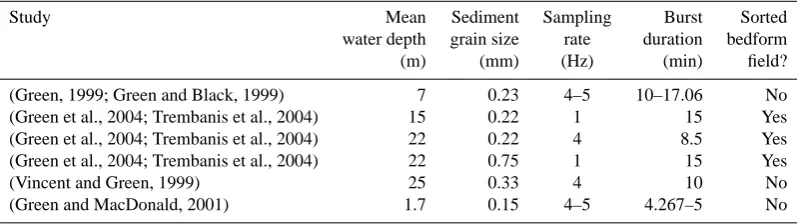
Study Mean Sediment Sampling Burst Sorted water depth grain size rate duration bedform
(m) (mm) (Hz) (min) field?
(Green, 1999; Green and Black, 1999) 7 0.23 4–5 10–17.06 No
(Green et al., 2004; Trembanis et al., 2004) 15 0.22 1 15 Yes
(Green et al., 2004; Trembanis et al., 2004) 22 0.22 4 8.5 Yes
(Green et al., 2004; Trembanis et al., 2004) 22 0.75 1 15 Yes
(Vincent and Green, 1999) 25 0.33 4 10 No
(Green and MacDonald, 2001) 1.7 0.15 4–5 4.267–5 No
“sorted bedforms” (Murray and Thieler, 2004; Coco et al., 2007a, b). The sorting feedback is initiated by wave-generated ripples whose size is a function of seabed compo-sition and hydrodynamic forcing conditions (e.g., Cummings et al., 2009). Regions covered with fine sediment support smaller wave-generated ripples than areas mantled by coarse sediment. Strong turbulence above the large wave ripples on coarse domains enhances the erosion of fine material from the bed (and also functions as a barrier to the deposition of suspended fine sediment). Near-bottom currents lead to the advection of suspended fine material and the preferential set-tling of suspended fine sediment in areas where the seabed is composed of predominantly fine sediment with small wave ripples (and correspondingly less turbulence induced by the smaller features). Through self-organization this local sort-ing feedback leads to spatially extensive features. The nu-merical model of Coco et al. (2007a) indicates that the sort-ing feedback operates in a wide range of forcsort-ing conditions (Coco et al., 2007b).
Sorted bedforms show several configurations that we di-vide into two distinct end-member patterns typified by the location of the coarse domain, either in the trough of the bed-form or on the flanks of the bedbed-forms (appearance on both the updrift and/or downdrift are possible; e.g., Goffet al., 2005; Ferrini and Flood, 2005). We note that within an in-dividual sorted bedform field the pattern configuration can change (Thieler et al., 2014; Ferrini and Flood, 2005). Pre-vious work with the finite-amplitude models by Murray and Thieler (2004) and Coco et al. (2007a) showed the presence of coarse domains solely on the downdrift flank of bedforms. While Coco et al. (2007b) did show the potential for coarse domains to occur in the trough of bedforms, this configu-ration was highly path dependent (i.e., the result of a high wave event that is preceding and followed by smaller waves). Van Oyen et al. (2010, 2011), through linear stability analy-sis, showed the presence of two pattern modes in the initial infinitesimal-amplitude instability that correspond to these two distinct configurations. However Van Oyen et al. (2010, 2011) showed that each pattern mode is the result of sep-arate feedback mechanisms, where coarse domains present in troughs occurred as the result of a flow–bathymetry
feed-back, while coarse domains present on bedform flanks is the result of the previously described sorting feedback (refereed to as the “roughness” feedback by Van Oyen et al. (2010, 2011).
With the goal of presenting a new hybrid model, we first describe the development of the near-bed suspended sedi-ment reference concentration predictor from the large data set of Green and colleagues (Green, 1996, 1999; Green and Black, 1999; Vincent and Green, 1999; Green and MacDon-ald, 2001; Green et al., 2004; Trembanis et al., 2004). We then outline the sorted bedform model and the modifications to incorporate the new data-driven components. This new model is meant as an update to the Coco et al. (2007a) model. The new predictors in the hybrid model are more accurate and better performing than the formulations used in the Coco et al. (2007a) model. Finally, we present a novel experiment with the new hybrid model to show autogenic behaviors that were not present in the Coco et al. (2007a) model (i.e., the ap-pearance of two pattern configurations solely from a sorting feedback) and discuss advantages and disadvantages of this data-driven approach.This paper does not attempt to quanti-tatively compare the new hybrid model against older model-ing efforts: instead we offer this new model as a refinement to the previous model that is additionally able to capture new dynamics.
2 GP methods
2.1 Data set
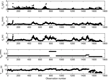
Figure 2 shows the multi-setting field data set composed of 1748 individual measurements from 6 separate field experi-ments at different locations in New Zealand. We briefly marize the experiments below and in Table 1; a detailed sum-mary of each experiment and the specific methodology used to determine the near-bed suspended sediment reference con-centration (C0; g L−1), significant near-bed orbital velocity
(Usig; m s−1), wave orbital diameter at the bed (d0; m), mean
grain size (d50; m), and mean spectral wave period at the bed
(Tmean; s) is available in the associated references. A single
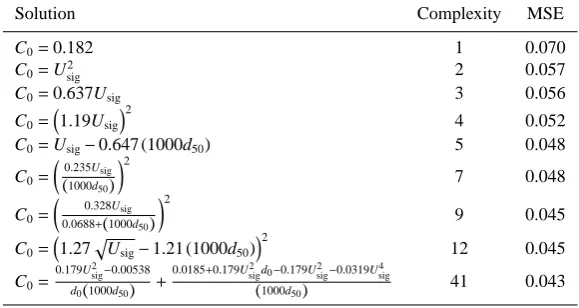
Table 2.Solutions for reference concentration.
Solution Complexity MSE
C0=0.182 1 0.070
C0=U2sig 2 0.057
C0=0.637Usig 3 0.056
C0=
1.19Usig
2
4 0.052
C0=Usig−0.647 (1000d50) 5 0.048
C0=
0.235U
sig
(1000d50)
2
7 0.048
C0=
0.328U
sig
0.0688+(1000d50)
2
9 0.045
C0=
1.27p
Usig−1.21 (1000d50)
2
12 0.045
C0= 0.179U2
sig−0.00538 d0(1000d50) +
0.0185+0.179U2
sigd0−0.179U2sig−0.0319Usig4
(1000d50) 41 0.043
depth of 7 m. Data from three experiments (Green et al., 2004; Trembanis et al., 2004) were collected from separate locations in a field of sorted bedforms (669, 126, and 554 measurements). A single instrument frame was located in a domain composed of coarse sand (22 m depth) and two in-strument frames were located in fine sand domains (15 and 22 m depth). The fifth experiment was deployed offof a head-land in 25 m of water depth (56 measurements; Vincent and Green, 1999). The final experiment in the database collected 241 measurements in a microtidal estuary in a mean water depth of 1.7 m (Green and MacDonald, 2001). All data were gathered in burst mode, with burst durations ranging from 4.267 to 17.06 min. In addition to the multiple settings and significant amount of data, this data set is ideal for applica-tion in the sorted bedform model because three of the six ex-periments in the composite data set are derived from a sorted bedform field (Green et al., 2004; Trembanis et al., 2004).
2.2 Selection of training, validation, and testing data sets
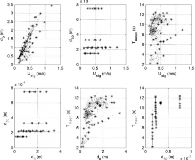
The database is split into three subsets to be used as train-ing, validation, and testing. The training data set is used to develop candidate solutions. The validation data set is used to evaluate the generality of a predictor, the fitness of GP-derived solutions against more data, and ultimately to deter-mine which predictors persist. The testing data set is unused and unseen by the GP algorithm; it is reserved as an inde-pendent test of the final predictors (and other published pre-dictors). Because our database does not cover the entirety of the forcing space with equal density (Fig. 3), the selec-tion and partiselec-tioning of data into these three categories is crucial for developing a well-performing predictor applica-ble to a range of environments (e.g., Bowden et al., 2002). The C0 data set is sparse in areas because of a lack of
col-lected data, while dense in other regions of phase space as a result of similar field settings, forcing conditions, and the number of data points collected in a given experiment. If the data are randomly divided, there is a potential that the
training data exclude data from sparse regions in the data set (i.e., coarse-grained and/or strong hydrodynamic data). How-ever, in the genetic programming literature we could find no proven “best practice” for selection of the data subsets or an optimal percentage of training, validation, and testing data (Kuschu, 2002; Panait and Luke, 2003; Gagné et al., 2006); we therefore use a technique that was successful in a previous study (Goldstein et al., 2013).
Informed data selection has been shown to produce better results with ML predictors than “blind” or random data se-lection (e.g., Bowden et al., 2002; May et al., 2010). In this study we select training data through the use of a maximum dissimilarity algorithm (MDA; Camus et al., 2011). This al-gorithm is not a clustering routine (where centroids denote a representative value of the data in the cluster), but is instead a selection routine (where a centroid represents the most dis-similar data point from the previous centroids; Camus et al., 2011). This selection routine allows the use of a minimum of training data that is able to capture the variance present in the entire data set while leaving the majority of the data to be utilized as validation and testing.
The maximum dissimilarity algorithm is described in Ca-mus et al. (2011) and we review the method. Selection starts with the linear normalization of the independent variables to a value between 0 (minimum value of a given variable) and 1 (maximum value of a given variable). A single data point, a “seed”, is selected as the first centroid. The algorithm then se-lects the additional centroids (the number determined by the user) through an iterative process: each data point is a four-dimensional vector (normalized Tmean, Usig, d0, d50 space)
and is associated with a distance to the nearest centroid. The single data point with the maximum distance between itself and the nearest centroid is selected as the next centroid (Ca-mus et al., 2011). The MDA routine continues until the user-defined number of centroids is reached and the data are then denormalized.
0 200 400 600 800 1000 1200 1400 1600 1800 0
2
C 0
(g/L)
0 200 400 600 800 1000 1200 1400 1600 1800
0 1 2
U si
g
(m/s)
0 200 400 600 800 1000 1200 1400 1600 1800
0 2 4
d 0
(m)
0 200 400 600 800 1000 1200 1400 1600 1800
0 0.5 1
d 50
(mm)
0 200 400 600 800 1000 1200 1400 1600 1800
0 10 20
T me
an
(s)
Observation number
Student Version of MATLAB
Figure 2.Observations of suspended sediment reference concentration data set C0 and concomitant measurements of significant wave
velocity at the bed (Usig), wave orbital excursion at the bed (d0), mean grain size of bed material (d50), and mean spectral wave period at the
bed (Tmean). Note that mean grain size of bed material is shown here in millimeters. A similar figure appears in Oehler et al. (2012).
a data set, especially continuous data (e.g., May et al., 2010; Goldstein et al., 2013). Selecting too many centroids can rob the validation and testing data sets of poorly represented data (e.g., large Tmean, Usig, d0, d50) and may tend to cause the GP
to produce overly complex predictors (e.g., Gonçalves and Silva, 2013; Oates and Jensen, 1997, 1998). The selection of too few centroids can leave the testing data with too few data points to capture the variability in the data set (Goldstein et al., 2013). We use 40 centroids for the prediction of C0
(cen-troid locations can be seen in Fig. 3), the same as Goldstein et al. (2013). Data selected as the centroid locations are used for the training data, while the remaining data are used for validation and testing data. The data set is split between val-idation and testing randomly, without using a selection rou-tine. The final breakdown for the data sets is∼2 % training,
∼49 % validation, and∼49 % testing.
2.3 Genetic programming
We operate on this data set using the ML technique of genetic programming (GP; Koza, 1992; Poli et al., 2008), where
can-didate solutions (i.e., randomly generated initial equations) are evaluated and subsequently modified by adjusting the in-dependent variables as well as the mathematical relationships between variables (i.e., the mathematical form). Independent variables used in this study to predict C0are Tmean, Usig, d0,
and d50. We use Tmean, Usig, and d0as separate independent
variables for input to the GP (though they are related) in an attempt to introduce no additional information about which of these parameters is most relevant. Mathematical operators used in this study are+(addition),−(subtraction),× (mul-tiplication),÷(division), and √(square root), as well as in-teger powers (e.g., x2, x3, etc.). We omit logical functions in this analysis (e.g., if-then-else) because we aim to develop a smooth final solution.
Candidate solutions are evaluated based on a “fitness func-tion”, a user-defined error metric that determines how well a given candidate fits the validation data. Mean squared error (MSE) is used as the fitness function:
MSE=
Pn
i=1(pi−bi)2
Figure 3.Visualization of the range of conditions in the C0data set. Each plot represents a two-dimensional projection of the entire data
set onto the set of axes shown. For instance, the first panel with data projected onto the d0−Usigplane shows no information about d50or
Tmean. Stars denote centroid locations (training data), while points denote unselected data (validation and testing). Note that centroids are
distributed throughout the data set.
where n is the sample size, p are the predicted values, and
b are the observed values. Candidate solutions that minimize
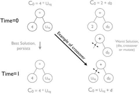
mean squared error are retained and poor performing solu-tions are discarded. Retained solusolu-tions are rearranged, com-bined, and manipulated in a probabilistic manner according to combinatorial processes: solutions “crossover” by com-bining elements of other solutions to develop a new solu-tion and “mutasolu-tions” develop new mathematical expression to substitute or tack on to a previous solution. Candidate so-lutions are commonly encoded in GP software as graphs or “trees”. The evolutionary processes that modify candidate solutions (change of variables and/or mathematical expres-sion) is accomplished by adjusting tree “limbs” (Fig. 4). Pre-dictors range from simple (small trees) to complex (large trees) as they are recombined in a variety of ways. The range of candidate solutions enables the searching of a large solu-tion space, and the search process continues until a solusolu-tion with zero error is found or the routine is halted.
In this study we use a proven software package developed by Schmidt and Lipson (2009, 2013). This software package,
“Eureqa”, outputs a suite of solutions with increasing math-ematical “complexity”, where complexity is a count of the numbers of operators and variables are used in the candidate solution. Each solution of a given complexity represents the equation with the least error compared to identically “com-plex” candidate solutions. Additionally, solutions must have less error compared to all previous less complex solutions. The line that traces the suite of solutions in complexity– fitness space is the “Pareto front”, and is a graphical rep-resentation of increasing fitness with increasing complexity. Many predictors along the Pareto front, from simple to com-plex, are retained in the solution set, requiring the user to pick a single solution as the final predictor of choice.
In the results presented here there is no single zero-error solution found; therefore we cease the search after roughly 1010formulas have been evaluated – continued search shows
Figure 4.Example of the genetic programming process. Potential solutions are encoded as a population of trees. Here a hypothetical population of two solutions is shown. The first solution has a low MSE and therefore persists to the next iteration. The second solu-tion has a high MSE and therefore is subject to removal, mutasolu-tion, or crossover. An example of “crossover” is shown here, whereby the old solution is combined with parts of other, better performing solutions to create a new potential solution in the next iteration.
techniques in parallel to determine a single appropriate solu-tion: (1) bias toward shorter, physically reasonable solutions, (2) examining “cliffs” in the Pareto front, and (3) examina-tion of soluexamina-tion fit.
Compact, simple solutions tend to offer more generaliza-tion power and are likely less overfitted (the minimum de-scription length principle; e.g., O’Neill et al., 2010). Addi-tionally, shorter solutions reappear with repeat initialization of the genetic programming algorithm, suggesting that these reappearing candidates represent the globally optimum so-lutions for a given function size. Longer soso-lutions do not tend to reappear, a result of a large search space that is not repeated during repeat initializations or the presence of multiple, equally optimal solutions in the large phase space (i.e., local minima). The inherent reproducibility of simple, weakly nonlinear solutions suggests their use as predictors until further data can be used to justify the use of highly non-linear predictors.
Areas along the Pareto front where large gains in predic-tion are obtained with small gains in solupredic-tion complexity, “cliffs”, are a natural place to observe potential solutions (Fig. 5). Schmidt and Lipson (2009) observed many phys-ically relevant solutions at the bottom of the last cliff of a given Pareto front, and therefore we focus our search for a final solution at the cliffs. Additionally, as candidate solu-tions are evaluated by minimizing error funcsolu-tions, solusolu-tions occasionally minimize mean squared error but are unphys-ical (e.g., functions that have poor extrapolation ability be-yond the domain of the training data). These solutions must be manually disregarded, as there is as yet no means of ex-cluding them.
Figure 5. Reference concentration Pareto front; MSE is mean squared error of candidate solution versus the validation data set. Complexity is a quantification of the candidate solution length (both mathematical operators and variables).
Once a single predictor is selected, it is evaluated using the independent testing data (data that the ML algorithm has not seen) with the normalized root-mean-squared error (NRMSE):
NRMSE=
√
MSE
b
, (2)
where b is the mean of the observed values. Additionally we report the correlation coefficient (Pearson’s r) for each predictor evaluated against the independent testing data. The NRMSE and correlation coefficient are also reported for the reference concentration predictor of Nielsen (1986) and Lee et al. (2004) evaluated against the independent testing data.
3 GP results
The GP algorithm output is shown in Table 2 (note that nu-merical coefficients listed in the table are dimensional). This experiment evaluated 1010 formulas to develop the Pareto front shown in Fig. 5. Cliffs occur along the Pareto front at complexities of 2, 4, 5, 9, and 41 (Fig. 5). Predictors gen-erally show nonlinear dependence on Usig/d50, qualitatively
similar to the predictors developed by Nielsen (1986) and Lee et al. (2004), which both show dependence on the modi-fied Shields parameter. We focus our analysis on the last cliff before the proliferation of very complex, nonlinear terms (so-lution 9):
C0=
0.328Usig
0.0688+(1000d50)
!2
. (3)
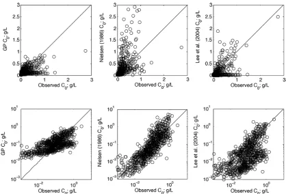
Figure 6.GP predictor of C0, Nielsen (1986) and Lee et al. (2004) predictor evaluated using only the independent testing data set. Top row
shows the predictors in linear space; bottom row shows log–log space.
compare the GP predictor as well as those developed by Nielsen (1986) and Lee et al. (2004): the NRMSE for each predictor is 1.1, 2.6, and 1.3, respectively, and the correla-tion coefficient is 0.58, 0.58, and 0.57, respectively. Results are shown in Fig. 6. The GP-derived predictor outperforms other predictors based on the NRMSE and is roughly iden-tical to the other predictors based on correlation coefficient. However, we note that at very low concentrations the perfor-mance of Eq. (3) deteriorates.
4 Hybrid sorted bedform model overview
We now incorporate this new C0predictor into a previously
described model of inner-shelf sorted bedforms developed by Coco et al. (2007a) that is based on the initial work of Murray and Thieler (2004). We briefly review the model below; a detailed treatment of the sediment transport rela-tions, hydrodynamic equations and their computational im-plementation are presented in Coco et al. (2007a). A three-dimensional model domain with periodic horizontal bound-ary conditions is used to represent a seabed composed of two grain sizes (dcoarse=0.0005 m and dfine=0.0002 m; fall
velocity wcoarse=0.07 m s−1 and wfine=0.02 m s−1). An
ini-tially flat bed (with slight bathymetric perturbation below 0.01 m) has a bulk composition of 70 % fine sediment and
30 % coarse sediment with individual cells that deviate from this ratio no more than 10 %. The model domain has a plan view size of 500 m×500 m, a vertical resolution of 0.05 m and a horizontal resolution of 5 m. Small-scale sorted bed-forms are modeled in the interest of computational efficiency (observed sorted bedforms range from the scale modeled to kilometers in plan view). In the experiments presented the initial water depth is 9 m, the wave period is 10 s, wave height is 2 m, the mean current is 0.2 m s−1, and the current is uni-directional. Sediment transport, computed independently for each size fraction, occurs only as suspended load and results in the change of bed elevation.
Suspended sediment transport is based on a simplified advection–diffusion framework, neglecting horizontal dif-fusion and assuming steady-state suspended sediment con-centration profiles (Murray and Thieler, 2004; Coco et al., 2007a). The flux of suspended sediment (qsusp,s), evaluated separately for each size fraction s, is the vertically integrated product of the current velocity profile (V(z)) and the sus-pended sediment concentration profile (Cs(z), where z is the
vertical coordinate) combined with a “morphodynamic dif-fusion” term to incorporate the role of bed slope (∇z) on
sed-iment transport:
qsusp,s=
Z
CsVdz−γs
1 5ws
γs=γc
16Eρ
3πws
Cd, (5)
where Uw is the maximum wave orbital speed at the bed
(m s−1; evaluated with linear wave theory), γ
c is the
mor-phodynamic diffusion coefficient,ρis the density of water,
Cd is the drag coefficient, and E is an efficiency factor (set
to 0.035). The integration of suspended sediment flux begins at the height where reference concentration is defined. The second term in Eq. (4) represents a “morphodynamic diff u-sion” term derived from energetics arguments (Bowen, 1980; Bailard, 1981). The calibration parameter in this framework isγcand is adjusted to maintain an order of magnitude diff
er-ence between the two terms on the right-hand side of Eq. (4), similar to the methodology of Calvete et al. (2001). For all experiments in this contribution,γc=0.07. The role of this
parameter is addressed further in the discussion section. Previous work by Coco et al. (2007a) demonstrates negli-gible sensitivity to different vertical current profile parame-terizations (i.e., descriptions that include current–wave inter-actions). In these experiments we use a logarithmic vertical current profile:
V (z)=1
κU
∗log z
z0
. (6)
where U∗is the shear velocity andκis the von Kármán
con-stant. The current profile begins at the roughness height z0,
which is related to wave-generated ripples (van Rijn, 1993):
z0=
1
30(2d50+28ηϑ), (7)
whereηis ripple height andϑis ripple steepness.
The wave-period-averaged vertical suspended sediment profile above wave-generated ripples (Cs) is calculated based
on Nielsen (1992):
Cs(z)=C0,se−
wsz
εs (8)
where C0,s is the near-bed reference concentration for grain size s and εs is the vertical sediment diffusivity. Coco et
al. (2007a) relied on the formulation developed by Nielsen (1986) to determine the near-bed reference concentration. We use the new GP-derived formulation developed in the previous section. To make the GP-derived C0predictor
com-patible with this model formulation, we assume Usig=Uw
and d50=ds, and therefore Eq. (3) becomes
C0=
0.328Uw
0.0688+(1000ds)
!2
. (9)
The reference concentration is applied at the height of the ripple crest, as in Coco et al. (2007a). In contrast to the work of Coco et al. (2007a) in this work we evaluate the sediment diffusion coefficient based on the work of Nielsen (1992):
εs= ΩksUw, (10)
where ksis the equivalent roughness andΩis a scaling coeffi -cient. Thorne et al. (2009) demonstrated that this parameter-ization underpredicts vertical sediment diffusivity by a factor of∼2 when using the original value ofΩ =0.016 suggested by Nielsen (1992). We therefore setΩ =0.032. Ripple pre-diction is performed using a new equilibrium scheme devel-oped using GP by Goldstein et al. (2013):
η= 0.313d0(1000d50)
1.12+2.18 (1000d50)
, (12)
ϑ= 3.42
22+
d0
1.12(1000d50)+2.18(1000d50)2
2. (13)
We evaluate the mean grain size at each model cell i (d50,i) at each time step as
d50,i= 1−Bcoarse,idfine+Bcoarse,idcoarse, (14)
where Bcoarse,i is the percentage of coarse sediment in the active layer at location i, and dfine and dcoarse are the
diam-eter of the fine and coarse fraction, respectively. An active layer vertically restricts sediment–flow interactions. All ex-periments presented here have a constant active layer thick-ness of 0.15 m. Sensitivity analyses performed by Coco et al. (2007a) demonstrate that the nature of the sorting feedback is not changed by modification of the active layer thickness.
5 Hybrid sorted bedform model results
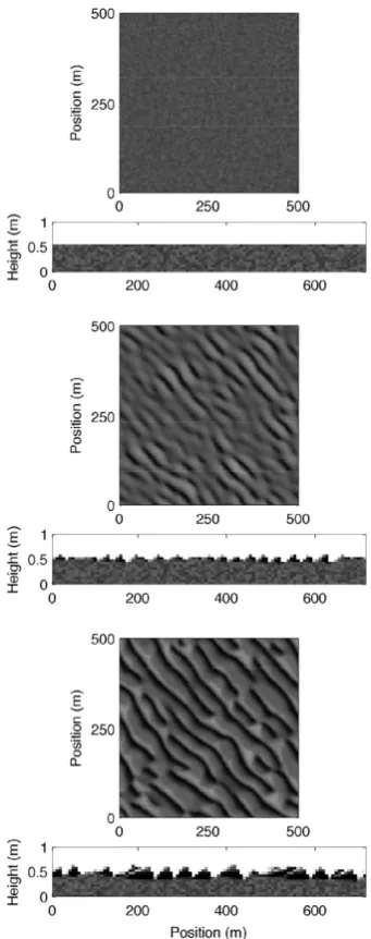
Figure 7.Plan view and profile view of sorted bedform model output (note the vertical exaggeration of profile view). Black and white pixels indicate fine (dfine=0.0002 m) and coarse (dcoarse=
0.0005 m) sediment, respectively. Current direction is from lower left to upper right and the profile is taken along this axis. The well-mixed and flat initial condition is shown in the top panels. Sorted bedforms appear within 50 days (middle panels) and are well de-veloped by model day 100 (bottom panels). These are mode 2 bed-forms; note that coarse domains appear on the updrift flank of the bedforms and wavelength and height are relatively small
are smaller), and therefore it tends to occupy the updrift flank of the bedform only.
Previous work by Coco et al. (2007a) showed the effect of variations in the size of the fine fraction while the coarse frac-tion size was held constant. In these experiments we evalu-ate the reverse: fine fraction diameter is held constant (dfine=
Figure 8.Variations in sorted bedform characteristics (wavelength and height) after 100 days when coarse grain size is held constant. No bedforms appear when the coarse material is too fine. Mode 1 bedforms (long wavelength, larger relief, coarse domains in trough) appear when coarse grain size is large and relatively immobile. Mode 2 bedforms (short wavelength, low relief, coarse domains on updrift flank) appear when coarse grain is between these two limits. No clear pattern was observed after 100 days when dcoarse=0.9 mm.
0.0002 m; wfine=0.02 m s−1), while the coarse fraction
diam-eter is varied between 0.0003 and 0.001 m (wcoarse=0.04–
0.12 m s−1). This range of sizes for the coarse fraction is
sim-ilar to the values found in sorted bedform fields worldwide (Coco et al., 2007b).
Results from this analysis can be seen in Fig. 8 (sorted bed-form wavelength and height are evaluated after 100 model days). Similar to Coco et al. (2007a) sorted bedforms do not appear when the grain size contrast between size fractions is too small (dfine/dcoarse<0.5). When coarse grains range from
0.004 to 0.008 m in diameter, larger coarse sediment tends to cause sorted bedforms to appear faster, decrease in wave-length, and increase in height. Within this range of grain sizes the coarse domain is located along the updrift flank and bed-forms migrate in the current direction.
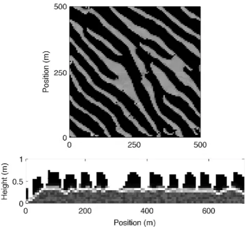
Figure 9.Plan view and profile view of mode 1 sorted bedforms after 50 days. Conditions are identical to Fig. 7 except dcoarse=
0.001 m. From identical initial conditions sorted bedforms appear much faster and are prominent features by 50 model days. Note that coarse domains appear solely in the bathymetric trough of the bed-forms and wavelength and height are relatively large.
suspended material is advected over the coarse domain (the bedform trough) and subsequently deposited on the updrift side of the following (downdrift) bedform.
In profile view a contiguous layer of coarse sediment ex-ists directly below the sorted bedform field (Fig. 9). This coarse layer occurs at the interface between the well-mixed sediment below (the undisturbed model initial conditions) and the reworked sediment above, a consequence of limited coarse sediment mobility and bedform migration (Goldstein et al., 2011). As bedforms migrate, the position of the sorted bedform trough changes. Fine sediment under the bedform trough, once too deep to experience fluid–sediment interac-tions, is excavated and suspended. Winnowing of fine sedi-ment and coarsening locally in the bedform trough, repeated as the bedforms migrate, results in the development of a hor-izontal layer of buried coarse sediment, a “sorting lag”.
In all results presented here, bedforms migrate and bed-form wavelength continues to grow through the model run and wavelength does not saturate. This perpetual coarsening of wavelength under conditions of unidirectional currents is identical to the behavior of the Coco et al. (2007b) and Mur-ray and Thieler (2004) model under unidirectional current forcing. (In the previous results, wavelength coarsening also occurs under the more realistic conditions of an asymmetri-cally reversing current, although coarsening is more gradual than under a unidirectional current.)
6.1 GP-derivedC0predictor
The newly developed C0 predictor has a nonlinear
depen-dence on d50 and Usig, similar to other previous empirical
predictors (Nielsen, 1986; Lee et al., 2004). This dependence is not imposed, but instead a result of the data sets used in the GP algorithm.
The GP reference concentration predictor relies on Usig,
while the sorted bedform model uses Uw. In the hybrid model
we assume Usig=Uw, where Uw is calculated from linear
wave theory. We direct the reader to other methods available to estimate Usigfrom surface wave parameters (e.g., Wiberg
and Sherwood, 2008). We force the sorted bedform model with a constant monochromatic wave field (height and pe-riod) to eliminate the chance that changes in wave charac-teristics influence the simulated seabed evolution. Therefore the assumption of Usig=Uwdoes not impact model results
shown here.
Ripple geometry was not used as an independent variable in the construction of the C0predictor. Dolphin and Vincent
(2009) recently suggested that ripple geometry may not aid in the prediction of C0, contrary to Nielsen (1986) and Green
and Black (1999). Though we do not have data to either sup-port or refute this claim, we can offer our results as an exam-ple of a well-performing prediction of reference concentra-tion without the explicit inclusion of ripple geometry. How-ever, the nonlinear nature of the reference concentration pre-diction and the constants embedded within Eq. (3) suggest that ripple configuration may be encoded within the predic-tor, either as a cause of the nonlinearity or a determinant of the constants.
The C0 predictor does not explicitly account for near-bed
currents that may be important mechanisms for enhancing suspension in sorted bedform fields (e.g., Gutierrez et al., 2005). The C0 predictor developed in this study is an
equi-librium predictor; therefore the role of time variance of C0is
sorted bedform model. This result is similar to previous work that suggests the Nielsen (1986) predictor may overestimate reference concentration (Bolaños et al., 2012; Thorne et al., 2002).
6.2 Hybrid sorted bedform model
The hybrid version of the sorted bedform model is able to reproduce the sorting feedback using new parameterizations built from data. The sorting feedback hypothesized by Mur-ray and Thieler (2004) is robust to changes in the mathemat-ical description of the processes in sediment transport and hydrodynamics on the continental shelf, and hybrid model results are comparable to previous modeling efforts (Mur-ray and Thieler, 2004; Mur(Mur-ray et al., 2005; Coco et al., 2007a). The behavior of the hybrid model and the Coco et al. (2007a) model under identical hydrodynamic forcing is dif-ferent because there are quantitative differences between the mathematical description of sediment transport processes. For instance, using the baseline conditions of the Coco et al. (2007a) model the hybrid model produces no sorted bed-forms. This is a direct result of changing the C0 predictor
from the Nielsen (1986) formula (which overpredicts sedi-ment transport; Fig. 6) to the new GP-derived C0predictor.
Changes to the sediment transport formulas prohibit us from directly comparing the three models under identical forcing conditions. Instead we offer this hybrid model as a refined version of the Coco et al. (2007a) model. The hybrid model has additional advantages beyond being more tightly coupled to observational data, most notably in favorable comparison to previous observational work.
Results shown in this contribution use two new prediction schemes based on GP (i.e., ripple morphology and reference concentration). We believe the new ripple prediction scheme of Goldstein et al. (2013) is an improvement over the previ-ous method used in the Coco et al. (2007a) model; however ripples in this model only significantly impact the vertical sediment diffusivity (εs) and the roughness height (z0). The
reference concentration, since it sets the magnitude of sus-pended sediment, is more strongly related to the new behav-iors in the model, and as a result we focus our analysis on the reference concentration.
Observational work has previously detected several dis-tinct varieties of sorted bedforms – those with coarse sedi-ment in the trough and those where coarse sedisedi-ment appears either in the trough and bedforms where coarse sediment is located on the flank (both the updrift and/or downdrift; e.g., Goffet al., 2005; Ferrini and Flood, 2005). Van Oyen et al. (2010, 2011) found that these two pattern configurations ap-pear in linear stability analysis as a result of two separate feedback mechanisms. Mode 1 bedforms (flow–topography feedback), where coarse domains are located in the bed-form trough, have a faster growth rate when waves and cur-rents are weaker and result in bedforms with longer wave-length, larger amplitude, and faster migration rates. Mode 2
bedforms (sorting or “roughness” feedback), where coarse grains appear along the updrift and downdrift flank of the bedform, have a faster growth rate when waves and currents are stronger and result in bedforms with smaller wavelengths, smaller heights, and slower migration rates. Yet results from linear stability analysis are applicable only at the scale of an infinitesimal perturbation.
Results from the finite-amplitude hybrid model also show that coarse domains can occur either on the updrift flank of the sorted bedform or collocated with the bedform trough, matching some aspects of previous observation work. How-ever instead of relying on two separate feedback mecha-nisms, the hybrid model is able to reproduce these two pat-tern configurations solely via the sorting mechanism. The presence of two distinct pattern modes occurs while current and wave conditions remain unchanged but coarse grain size is varied. When coarse grains are smaller (essentially iden-tical to increasing wave conditions in terms of increasing coarse sediment mobility) bedforms conform to the descrip-tion of the mode 2 features of Van Oyen et al. (2010, 2011) with smaller features, slower migration rates, and coarse sediment along the updrift flank of bedforms. When coarse grains are larger (essentially identical to decreasing wave conditions in terms of decreasing coarse sediment mobility) bedforms show characteristics of the mode 1 features of Van Oyen et al. (2010, 2011) with larger bedforms, faster migra-tion rates, and coarse sediment in the bedform trough. We again note this behavior occurs solely from a sorting feed-back. Bedform wavelength continues to grow in all model results shown here as a result of unidirectional current. How-ever, results in this contribution show that, for any given in-stant in model time, modeled sorted bedform patterns dis-play relatively homogenous wavelength and height (similar to Coco et al. (2007a) and Murray and Thieler (2004)). Ob-servational work shows sorted bedform fields have a well-defined pattern scale (i.e., a similar height and wavelength throughout the entire bedform field; see the compilation of observed bedform features in Coco et al. (2007b) for more details). It remains unknown whether the well-defined pat-tern scale of observed sorted bedforms reflects a saturated (steady state) wavelength or the uniformity of bedform wave-length and height at a given moment of pattern evolution.
lin-develop as result of the sorting feedback operating at finite amplitude. Future work with more detailed hydrodynamic parameterizations could shed light on the interplay between flow–bathymetry interactions and the sorting feedback in the mode 1 regime at finite amplitudes. However, these results do suggest that the finite-amplitude hybrid model may be able to capture the dynamics observed in the field. The presence of two distinct pattern modes in the hybrid model is a direct result of incorporating new data-driven parameterizations of the sediment transport process. In this contribution we ex-plore only one specific mechanism that results in mode 1 sorted bedforms, increasing the diameter of the coarse grain size fraction. There are likely other mechanism by which mode 1 bedforms may develop instead of mode 2 bedforms, notably by increasing water depth, decreasing wave forcing, or decreasing current velocity.
There are additional pattern-scale consequences to adjust-ing the sediment transport formulations. The new C0
predic-tor requires energetic conditions to move coarse sediment. This matches the observations and interpretations of Green et al. (2004), Trembanis et al. (2004), and Trembanis and Hume (2011), who suggest that energetic conditions are the only time when the coarse sediment of sorted bedforms is mobile. However lower coarse sediment mobility results in the cre-ation of more pattern defects, a common feature of field ex-amples of sorted bedforms (e.g., Fig. 1). Furthermore, after the work of Werner and Kocurek (1997, 1999), defects have been recognized as a fundamental variable in pattern-scale dynamics of bedforms (Huntley et al., 2008; Maier and Hay, 2009; Goldstein et al., 2011; Skarke and Trembanis, 2011). The presence of additional defects in the hybrid model may exert fundamental controls on pattern evolution.
The hybrid model is able to reproduce sorting feedback and two pattern modes when successfully calibrated. Cali-bration is accomplished by adjusting the variableγc in the morphodynamic diffusion term, Eqs. (4) and (5). The re-sults shown in this contribution haveγc=0.07. The sorting feedback and the development of two sorted bedform pat-tern modes occur in the range ofγc=0.05–0.08. This range contrasts with the work of Coco et al. (2007a, b), where the γc term could be adjusted at least one order of magnitude. This more limited calibration is the result of using multiple nonlinear elements in the construction of the model. Specifi-cally the morphodynamic diffusion term (thatγcmodifies) is highly nonlinear (i.e.,∝U5
w) and is built from energy-based
theory (Bowen, 1980; Bailard, 1981). Coco et al. (2007a) re-lied on a parameterization of C0 that scaled with U6w, eff
ec-tively scaling the two terms of Eq. (4) in a similar manner. In contrast our new C0 predictor scales with Uw2, and therefore
does not scale in a similar manner to the morphodynamic term (U5
w). We suggest that this mismatch, coupled with the
strong forcing condition that is required to move sediment in the model (i.e., large Uw), has lead to a smaller
permissi-ble parameter space where the morphodynamic term and the
permissible parameter space by the scaling argument made previously by Calvete et al. (2001): γc should be set to a value that maintains the ratio between the two terms on the right side of Eq. (4) to∼1 order of magnitude. Ifγcis set too high, the slope-dependent term is too strong and no bathy-metric perturbations develop. Ifγcis set too low, nonphysi-cally steep bathymetric perturbations develop. These results highlight the need to test the Bailard (1981) term in a range of conditions to see whether this description (or others) is valid. Though this morphodynamic diffusion term is often used in morphodynamic models, we could find no instance where this term has been tested in a wide range of conditions. Finally, the promising results of data-driven parameter-izations as components in the sorted bedform model sug-gests that this approach could be extended to other mor-phodynamic models and other parameterizations. A specific example from this work is the parameterization of vertical sediment diffusivity (or, more generally, the shape function that described the vertical suspended sediment concentra-tion profile). Recent work has begun to investigate the fast scale dynamics of vertical sediment diffusion over ripples (e.g., Davies and Thorne, 2005; van der Werf et al., 2007; O’Hara Murray et al., 2011) and how best to parameter-ize this process in large-scale coastal models (Amoudry and Souza, 2011; Amoudry et al., 2013). Traditional equilibrium parameterizations have also been evaluated with newly col-lected data (e.g., Thorne et al., 2002, 2009; Bolaños et al., 2012). More data, collected in a range of conditions, would enable a data-driven approach to the parameterization of the vertical suspended sediment profile shape.
7 Conclusion
Acknowledgements. We thank Paula Camus for sharing her clustering algorithm and to Terry Hume (NIWA, NZ) for pro-viding the image of Tairua Beach, NZ, bedforms seen in Fig. 1. E. B. Goldstein thanks “IH Cantabria” for funding during his stay, where this work was started. G. Coco acknowledges funding from the Cantabria Campus Internacional (Augusto Gonzalez Linares program). We thank an anonymous reviewer and Tomas Van Oyen for stimulating comments that improved the manuscript.
Edited by: F. Metivier
References
Amoudry, L. O. and Souza, A. J.: Deterministic coastal morpholog-ical and sediment transport modeling: A review and discussion, Rev. Geophys., 49, RG2002, doi:10.1029/2010RG000341, 2011. Amoudry, L. O., Bell, P. S., Thorne, P. D., and Souza, A. J.: To-ward representing wave-induced sediment suspension over sand ripples in RANS models, J. Geophys. Res.-Oceans, 118, 1–15, 2013.
Bailard, J. A.: An energetics total load sediment transport model for a plane sloping beach, J. Geophys. Res., 86, 10938–10954, 1981. Baptist, M. J., Babovic, V., Uthurburu, J. R., Keijzer, M., Uittenbo-gaard, R. E., Mynett, A., and Verwey, A.: On inducing equations for vegetation resistance, J. Hydraul. Res., 45, 435–450, 2007. Bolaños, R., Thorne, P. D., and Wolf, J.: Comparison of
measure-ments and models of bed stress, bedforms and suspended sedi-ments under combined currents and waves, Coast. Eng., 62, 19– 30, 2012.
Bowden, G. J., Maier, H. R., and Dandy, G. C.: Optimal division of data for neural network models in water resources applications, Water Resour. Res., 38(2), 2-1–2-11, 2002.
Bowen, A. J.: Simple models of nearshore sedimentation: Beach profiles and long-shore bars, in: The Coastline of Canada, edited by: McCann, S. B., 111 pp., Geol. Surv. of Can., Ottawa, 1980. Cacchione, D. A., Thorne, P. D., Agrawal, Y., and Nidzieko, N. J.:
Time-averaged near-bed suspended sediment concentrations un-der waves and currents: comparison of measured and model esti-mates, Cont. Shelf Res., 28, 470–484, 2008.
Calvete, D., Falqués, A., de Swart, H. E., and Walgreen, M.: Modelling the formation of shoreface-connected sand ridges on storm-dominated inner shelves, J. Fluid Mech., 441, 169–193, 2001.
Camus, P., Mendez, F. J., Medina, R., and Cofiño, A. S.: Analysis of clustering and selection algorithms for the study of multivariate wave climate, Coast. Eng., 58, 453–462, 2011.
Coco, G., Murray, A. B., and Green, M. O.: Sorted bedforms as self-organized patterns: 1. Model development, J. Geophys. Res., 112, F03015, doi:10.1029/2006JF000665, 2007a.
Coco, G., Murray, A. B., Green, M. O., Thieler, E. R., and Hume, T. M.: Sorted bedforms as self-organized patterns: 2. Complex forcing scenarios, J. Geophys. Res., 112, F03016, doi:10.1029/2006JF000666, 2007b.
Corzo, G. A., Solomatine, D. P., Hidayat, de Wit, M., Werner, M., Uhlenbrook, S., and Price, R. K.: Combining semi-distributed process-based and data-driven models in flow simulation: a case study of the Meuse river basin, Hydrology and Earth System Sci-ences, 13, 9, 1619–1634, 2009.
Cummings, D. I., Dumas, S., and Dalrymple, R. W.: Fine-grained versus coarse-grained wave ripples generated experimentally un-der large-scale oscillatory flow, J. Sediment. Res., 79, 83–93, 2009.
Davies, A. G. and Thorne, P. D.: Modeling and measurement of sed-iment transport by waves in the vortex ripple regime, J. Geophys. Res., 110, C05017, doi:10.1029/2004JC002468, 2005.
Dolphin, T. and Vincent, C. E.: The influence of bed forms on ref-erence concentration and suspension under waves and currents, Cont. Shelf Res., 29, 424–432, 2009.
Ferrini, V. L. and Flood, R. D.: A comparison of rippled scour de-pressions identified with multibeam sonar: Evidence of sediment transport in inner shelf environments, Cont. Shelf Res., 25, 1979– 1995, 2005.
Gagné, C., Schoenauer, M., Parizeau, M., and Tomassini, M.: Ge-netic programming, validation sets, and parsimony pressure, in: Genetic Programming, 9th European Conference, EuroGP2006, Lecture Notes in Computer Science, LNCS 3905, edited by: Col-let, P., Tomassini, M., Ebner, M., Gustafson, S., and Ekárt, A., Springer, Berlin, Heidelberg, New York, 2006, 109–120, 2006. Goff, J. A., Mayer, L. A., Traykovski, P., Buynevich, I., Wilkens, R.,
Raymond, R., Glang, G., Evans, R. L., Olson, H., and Jenkins, C.: Detailed investigation of sorted bedforms, or “rippled scour depressions”, within the Martha’s Vineyard Coastal Observatory, Massachusetts, Cont. Shelf Res., 25, 461–484, 2005.
Goldstein, E. B., Murray, A. B., and Coco, G.: Sorted bed-form pattern evolution: Persistence, destruction and self-organized intermittency, Geophys. Res. Lett., 38, L24402, doi:10.1029/2011GL049732, 2011.
Goldstein, E. B., Coco, G., and Murray, A. B.: Prediction of wave ripple characteristics using genetic programming, Cont. Shelf Res., 71, 1–15, 2013.
Gonçalves, I. and Silva, S.: Balancing Learning and Overfitting in Genetic Programming with Interleaved Sampling of Training Data, in: EuroGP 2013. LNCS, edited by: Krawiec, K., Moraglio, A., Hu, T., Etaner-Uyar, A., and Hu, B., Springer, Heidelberg, 7831, 73–84, 2013.
Gonçalves, I., Silva, S., Melo, J., and Carreiras, J.: Random Sam-pling Technique for Overfitting Control in Genetic Program-ming, in: EuroGP 2012. LNCS, edited by: Moraglio, A., Silva, S., Krawiec, K., Machado, P., and Cotta, C., Springer, Heidel-berg, 7244, 218–229, 2012.
Green, M.: Introducing ALICE, Water and Atmosphere, 4, 8–10, 1996.
Green, M. O.: Test of sediment initial-motion theories using irregular-wave field data, Sedimentology, 46, 427–441, 1999. Green, M. O. and Black, K. P.: Suspended-sediment reference
con-centration under waves: field observations and critical analysis of two predictive models, Coast. Eng., 38, 115–141, 1999. Green, M. O. and MacDonald, I. T.: Processes driving estuary
in-filling by marine sands on an embayed coast, Mar. Geol., 178, 11–37, 2001.
Green, M. O., Vincent, C. E., and Trembanis, A. C.: Suspension of coarse and fine sand on a wave-dominated shoreface, with impli-cations for the development of rippled scour depressions, Cont. Shelf Res., 24, 317–335, 2004.
of “defects” on sorted bedform dynamics, Geophys. Res. Lett., 35, L02601, doi:10.1029/2007GL030512, 2008.
Karunarathna, H. and Reeve, D. E.: A hybrid approach to model shoreline change at multiple timescales, Cont. Shelf Res., 66, 29– 35, 2013.
Kitsikoudis, V., Sidiropoulos, E., and Hrissanthou, V.: Derivation of Sediment Transport Models for Sand Bed Rivers from Data-Driven Techniques, in: Sediment Transport Processes and Their Modelling Applications, edited by: Manning, A., ISBN: 978-953-51-1039-2, InTech, doi:10.5772/53432, 2013.
Knaapen, M. A. F. and Hulscher, S. J. M. H. : Regeneration of sand waves after dredging, Coast. Eng., 46, 277–289, 2002.
Knaapen, M. A. F. and Hulscher, S. J. M. H.: Use of a genetic al-gorithm to improve predictions of alternate bar dynamics, Water Resour. Res., 39, 1231, doi:10.1029/2002WR001793, 2003. Koza, J. R.: Genetic Programming, On the Programming of
Com-puters by Means of Natural Selection, MIT Press, Cambridge, MA, USA, 1992.
Krasnopolsky, V. M. and Fox-Rabinovitz, M. S.: A new synergetic paradigm in environmental numerical modeling: Hybrid mod-els combining deterministic and machine learning components, Ecol. Model., 191, 5–18, 2006.
Kushchu, I.: An evaluation of evolutionary generalisation in genetic programming, Artif. Intell. Rev., 18, 3–14, 2002.
Lee, G., Dade, W. B., Friedrichs, C. T., and Vincent, C. E.: Examination of reference concentration under waves and cur-rents on the inner shelf, J. Geophys. Res., 109, C02021, doi:10.1029/2002JC001707, 2004.
Maier, I. and Hay, A. E.: Occurrence and orientation of anor-bital ripples in near-shore sands, J. Geophys. Res., 114, F04022, doi:10.1029/2008JF001126, 2009.
May, R. J., Maier, H. R., and Dandy, G. C.: Data splitting for artifi-cial neural networks using SOM-based stratified sampling, Neu-ral Networks, 23, 283–294, 2010.
Murray, A. B. and Thieler, E. R.: A new hypothesis and exploratory model for the formation of large-scale inner-shelf sediment sort-ing and “rippled scour depressions”, Cont. Shelf Res., 24, 295– 315, 2004.
Murray, A. B., Coco, G., Green, M. O., Hume, T., and Thieler, E. R.: Different approaches to modeling inner shelf sorted bedforms, in: Proceedings of the Conference “River, Coastal and Estuarine Morphodynamics”, edited by: Parker, G. and Garcia, M., Taylor and Francis, London, 1009–1015, 2005.
Nielsen, P.: Suspended sediment concentrations under waves, Coast. Eng., 10, 23–31, 1986.
Nielsen, P.: Coastal Bottom Boundary Layers and Sediment Trans-port, World Sci., Singapore, 1992.
Oates, T. and Jensen, D.: The effects of training set size on deci-sion tree complexity, Proceedings of the Fourteenth International Conference on Machine Learning, Madison, WI, Morgan Kauf-mann, 254–262, 1997.
Oates, T. and Jensen, D.: Large datasets lead to overly complex models: An explanation and a solution, Proceedings of the Fourth International Conference on Knowledge Discovery and Data Mining, New York, NY, AAAI Press, 294–298, 1998.
Oehler, F., Coco, G., Green, M. O., and Bryan, K. R.: A data driven approach to predict suspended-sediment reference concentration under non-breaking waves, Cont. Shelf Res., 46, 96–106, 2012.
trawave observations of sediment entrainment processes above sand ripples under irregular waves, J. Geophys. Res., 116, C01001, doi:10.1029/2010JC006216, 2011
O’Neill, M., Vanneschi, L., Gustafson, S., and Banzhaf, W.: Open issues in genetic programming, Genet. Program. Evol. M., 11, 339–363, 2010.
Panait, L. and Luke, S.: Methods for Evolving Robust Programs, in: Genetic and Evolutionary Computation-GECCO 2003, Vol. 2724, no. 66, Berlin, Heidelberg, Springer Berlin Heidelberg, 1740–175, 2003.
Pape, L., Ruessink, B. G., Wiering, M. A., and Turner, I. L.: Re-current neural network modeling of nearshore sandbar behavior, Neural Networks, 20, 509–518, 2007.
Pape, L., Kuriyama, Y., and Ruessink, B. G.: Models and scales for cross-shore sandbar migration, J. Geophys. Res., 115, F03043, doi:10.1029/2009JF001644, 2010.
Poli, R., Langdon, W. B., and McPhee, N. F.: A field guide to ge-netic programming, Lulu Enterprises Uk Limited, 2008 Ruessink, B. G.: Calibration of nearshore process models:
Applica-tion of a hybrid genetic algorithm, J. Hydroinformatics, 7, 135– 149, 2005.
Schmidt, M. and Lipson, H.: Distilling free-form natural laws from experimental data, Science, 324, 81–85, 2009.
Schmidt, M. and Lipson, H.: Eureqa (Version 0.98 beta) [Software], available at: http://www.eureqa.com/, 2013.
Skarke, A. and Trembanis, A. C.: Parameterization of bedform mor-phology and defect density with fingerprint analysis techniques, Cont. Shelf Res., 31, 1688–1700, 2011.
Thieler, E. R. Foster, D. S., Himmelstoss, E. A., and Mallinson, D. J.: Geologic framework of the northern North Carolina, USA in-ner continental shelf and its influence on coastal evolution, Mar. Geo., 348, 113–130, 2014.
Thorne, P. D., William, J. J., and Davies, A. G.: Suspended sedi-ments under waves measured in a large scale flume facility, J. Geophys. Res., 107, 4.1–4.16, 2002.
Thorne, P. D., Davies, A. G., and Bell, P. S.: Observations and analysis of sediment diffusivity profiles over sandy rip-pled beds under waves, J. Geophys. Res., 114, C02023, doi:10.1029/2008JC004944, 2009.
Trembanis, A. C. and Hume, T. M.: Sorted bedforms on the inner shelf offnortheastern New Zealand: spatiotemporal relationships and potential paleo-environmental implications, Geo-Mar Let-ters, 31, 203–214, 2011.
Trembanis, A. C., Wright, L. D., Friedrichs, C. T., Green, M. O., and Hume, T.: The effects of spatially complex inner shelf rough-ness on boundary layer turbulence and current and wave friction: Tairua embayment, New Zealand, Cont. Shelf Res., 24, 1549– 1571, 2004.
van der Werf, J. J., Doucette, J. S., Donoghue, T., and Ribberink, J. S.: Detailed measurements of velocities and suspended sand con-centrations over full?scale ripples in regular oscillatory flow, J. Geophys. Res., 112, F02012, doi:10.1029/2006JF000614, 2007. van Maanen, B., Coco, G., Bryan, K. R., and Ruessink, B. G.: The use of artificial neural networks to analyze and predict along-shore sediment transport, Nonlin. Processes Geophys., 17, 395– 404, 2010,
Van Oyen, T., de Swart, H. E., and Blondeaux, P.: Bottom topog-raphy and roughness variations as triggering mechanisms to the formation of sorted bedforms, Geophys. Res. Lett., 37, L18401, doi:10.1029/2010GL043793, 2010.
Van Oyen, T., de Swart, H. E., and Blondeaux, P.: Formation of rhythmic sorted bed forms on the continental shelf: an idealised model, J. Fluid Mech., 684, 475–508, 2011.
van Rijn, L. C.: Principles of Sediment Transport in Rivers, Estuar-ies and Coastal Seas, Aqua, Amsterdam, 1993.
Vincent, C. E. and Green, M. O.: The control of resuspension over megaripples on the continental shelf, in: Proceedings of Coastal Sediments 99, New York, USA, ASCE, 269–280, 1999. Vincent, C. E. and Hanes, D. M.: The accumulation and decay of
near-bed suspended sand concentration due to waves and wave groups, Cont. Shelf Res., 22, 1987–2000, 2002.
Werner, B. T. and Kocurek, G.: Bedform dynamics: Does the tail wag the dog?, Geology, 25, 771–774, 1997.
Werner, B. T. and Kocurek, G.: Bedform spacing from defect dy-namics, Geology, 27, 727–730, 1999.
Wiberg, P. L. and Sherwood, C. R.: Calculating wave-generated bot-tom orbital velocities from surface-wave parameters, Comput. Geosci., 34, 1243–1262, 2008.