Some improvements in subbasalt imaging using pre-stack depth migration

(1)

www.solid-earth.net/2/1/2011/ doi:10.5194/se-2-1-2011

Solid Earth

Some improvements in subbasalt imaging using pre-stack

depth migration

I. Flecha1, R. Carbonell1, R. W. Hobbs2, and H. Zeyen3

1_{Departament de Geof´ısica i Tectònica, Institut de Ciències de la Terra “Jaume Almera”-CSIC,} C/ Lluis Solé i Sabaris s/n, 08028 Barcelona, Spain

2_{Department of Earth Sciences, University of Durham, Durham DH1 3LE, UK}

3_{Departement des Sciences de la Terre, Universite de Paris-Sud, Bat. 503, 91405 Orsay Cedex, France} Received: 29 December 2009 – Published in Solid Earth Discuss.: 8 February 2010

Revised: 8 November 2010 – Accepted: 22 November 2010 – Published: 3 January 2011

Abstract. Subbasalt imaging can be improved by carefully applying pre-stack depth migration. Pre-stack depth migra-tion requires a detailed velocity model and an accurate trav-eltime calculation. Ray tracing methods are fast but, often fail in calculating traveltimes in complex models, specially, when they feature high velocity contrasts. Finitte difference solutions of the eikonal are more stable and can produce a traveltime field for the whole model avoiding shadow zones. A synthetic test was carried out to check the performance of a new pre-stack depth migration algorithm in a model that features a high velocity layer surrounded by lower veloci-ties. The results reasonably reproduce the original model. The same scheme was used to process long-offset reflec-tion data from the Faroe Shelf where convenreflec-tional techniques (stack) were insufficient to assess the structure under a basalt layer. Pre-stack depth migration produced an improved im-age which recovered the main features in the stacked section and allowed to identify some subbasalt coherent events.

1 Introduction

Seismic imaging comprises a wide range of methodologies. Among these techniques, the most common in geophysical prospecting is seismic reflection, which has provided valu-able data to infer the subsurface structure. Seismic reflec-tion principles are based on approximareflec-tions that simplify the imaging problem, two of the most restrictive are: the Earth is considered as a sequence of homogeneous subhorizontal lay-ers and interfaces between laylay-ers consist in a vertically sharp

Correspondence to: I. Flecha

([email protected])

and laterally smooth discontinuity (Yilmaz, 1987). Process-ing flows deduced from these premises generate detailed im-ages in layered and laterally homogeneous media. However, in nature, there are often geological settings where these as-sumptions fail dramatically, and the methodology based on them is going to be insufficient. This is the case in basalt covered areas and beneath salt instrusions. The presence of a high-velocity and highly heterogeneous layer (basalt) em-bedded in low-velocity sediments, has a detrimental effect on imaging beneath this structure (Martini and Bean, 2002). The basalt acts as a barrier for seismic signal. Most of the en-ergy reflects or travels along this layer, therefore little enen-ergy goes through the basalt layer. In addition, the backscattered energy that returns to the surface from basalt and subbasalt structures features a lack of coherence caused by the irregular interfaces of the basaltic body and the heterogeneities within the basalt itself. Hence, in this cases a more sophisticated approach, such as pre-stack depth migration, is needed.

The North Atlantic province has been widely studied by the oil industry. Standard seismic imaging techniques have been succesfully applied for many years in the sedimentary basins located in this area. The Faroe-Shetland Basin repre-sents a potential hydrocarbon reservoir ready for exploration. To the center of the basin, geology is well known but, in the NW region, sequences of basalt cover underlying structures and make exploration both challenging and risky (Sørensen, 2003). In the present study, a new pre-stack depth migration scheme was implemented to address the subbasalt imaging problem. This manuscript shows the improvements obtained by this pre-stack depth migration approach applied to data acquired over the Faroe Shelf.

(2)

2 I. Flecha et al.: Some improvements in subbasalt imaging using pre-stack depth migration 2 Geological and geophysical setting

In the Faroe-Shetland Basin, huge amounts of basaltic rock were erupted during the Paleocene-Eocene. Previous studies suggest this basalt is covering relatively low velocity materi-als which may be sediments (Hughes et al., 1998; Richardson et al., 1999; Fliedner and White, 2003; Raum et al., 2005). Topography before the emplacement of the basalt was dom-inated by normal faults as a consequence of extension and subsidence during the Cretaceous and Paleocene (Richard-son et al., 1999). Basaltic flows extended over long dis-tances in the basin after filling the lows between fault blocks. This causes an irregular bottom basalt interface. Basalt was erupted in different episodes. Three major basalt units have been identified: Lower, Middle and Upper Series. Their thicknesses and compositions differ from one unit to an-other (Noe-Nygaard and Rasmussen, 1968). Although, the basalt flow stratigraphy in this area is mainly layered, it in-cludes tuffs and breccias increasing the inner velocity con-trasts (Maresh and White, 2005). Moreover, in periods with-out igneous activity, lacustrine shales and coals were accu-mulated and sediments were emplaced filling the basin floor deeps (White et al., 2003). Those facts result in a highly heterogeneous distribution of physical properties within the basaltic body.

In the Faroe Shelf, the structure above the basalt and the top basalt interface can be succesfully resolved using con-ventional techniques because of the high contrast in physical properties between basalt and overlying sediments. How-ever, attenuation and scattering of the seismic wavefield as it passes through the basaltic pile make seismic imaging dif-ficult below the top basalt surface (Smallwood et al., 2001). The top basalt interface shows an irregular topography fea-turing fractal properties (Martini and Bean, 2002). This ir-regular topography is often at a scale similar to the seis-mic wavelength which causes the dispersion of elastic energy (scattering) degrading the signal coherence in the wavefield. In addition, heterogeneities within the basalt flows yield a high impedance contrast generating internal reverberations, mode conversions and internal multiples (Martini and Bean, 2002). Therefore, seismic energy reflected or refracted by these structures is incoherently scattered and dispersed re-sulting in a poor subbasalt image.

3 Pre-stack depth migration

An extensive revision of the algorithms and evolution of Pre-Stack migration can be found in the dedicated volume of Jones et al. (2008). Pre-stack depth migration aims to place the reflected amplitude at the precise location within the model from which the energy was reflected. Conven-tional migration algorithms requiere travel time tables to dis-tribute the energy recorded (the amplitude of the seismo-grams) among the grid points in the model. The amplitudes of a trace in a shot gather, a(ti), are distributed (sprayed)

among the points of a gridded model according to theti time at which it arrived at the sensor. Therefore, an algorithm to compute the travel times is imperative in order to be able to migrate. There are different ways to compute this travel times. A large majority of algorithms use conventional ray tracing approximations in one of each varieties, ray shoot-ing, two point ray tracshoot-ing, gausian beam etc. Once the travel time has been estimated we need to estimate how the am-plitude is distributed among all the grid points in the model. The amplitude in the trace can be considered to be:

a(ti) = X

j

rj · a(ti)j

wherej covers all the points of the model characterized by a timeti.ti is the time it took the seismic energy to travel from the source to that point in the model and then to the receiver. The calculation of traveltime tables for a given velocity model is an essential stage in Kirchhoff prestack depth mi-gration. Classical ray tracing techniques have been widely used to solve the forward problem (Zelt and Smith, 1992) and to calculate traveltime tables. Snell’s law based algo-rithms are fast and provide an estimation of the traveltime for areas in the model sampled by rays traced. However, in some implementations, sampling all the model requires a large amount of rays and depending on the velocity model (e.g. high velocity gradients) some areas can be undersam-pled resulting in shadow zones where no traveltimes are cal-culated. Ray-tracing methods in the presence of high velocity contrasts, and/or structures with sharp edges have difficulties in calculating the travel times. The result is that a few grid points lack travel times. This can be solved in different ways, for example by performing interpolating schemes (see Jones et al., 2008 for a review) or by using a finite difference ap-proach.

In the present work, we used a finite difference algorithm to solve the eikonal equation (Hole and Zelt, 1995). Using this algorithm, traveltimes are calculated for every node in the model, which slightly increases the computational cost compared with shooting ray methods, but, on the other hand, shadow zones are avoided. Moreover, using complete trav-eltime tables allows the handling of diffractions, correctly restoring the diffracted energy to its original position in the model. The finite difference solution of the eikonal equation is not unique to the algorithm used in this manuscript. This approach is used in other commercial packages. The advan-tages of using the eikonal to compute the travel times is that it is more robust than ray tracing methods as it is able to es-timate travel times for all the points in a model grid being more stable when high velocity contrasts exist.

As migration consist of summation of the contributions from the wavefield for every source-receiver pair, once the traveltime field has been calculated, a half-derivative is per-formed on every trace and amplitudes are spread among the grid points of the model. The amplitudes have been

(3)

I. Flecha et al.: Some improvements in subbasalt imaging using pre-stack depth migration 3

4 I. Flecha et al.: Some improvements in subbasalt imaging using pre-stack depth migration

0

0.5

1.0

1.5

Depth(km)

0 1 2 3 4 5

Distance (km) 1.5 1.7 1.9 2.1 2.3 V elocity(km/s) 0 1 2 3 T ime(s)

0 1 2 3 4 5

Distance (km)

Figure 1.Velocity model used to calculate synthetic data (top) and a shotgather generated at x=4 km (bottom).

Computing obliquity factors by using the forward model-ing parameters, as the angle of incidence at each of the model grid point is the conventional approach. The algorithm, in this manuscript in its present form uses the semblance of the tau-p transform of the shot gathers. The most relevant dif-ference between the conventional algorithms and the current

one is that conventional schemes use to compute therjusing

the model (they are model dependent) while in the approach used in this manuscript we use the actual data to compute the obliquity factors (the algorithm is data dependent). The sem-blance of the tau-p transform of the shot gathers represents a measure of the reflected energy as a function of the slowness (ray parameter, direction of the reflection). Therefore, these are representative of the obliquity factors.

Another key point in pre-stack depth migration is the gen-eration of numerical artifacts that result in “smiling” images. This is a known issue that usually is solved by limiting the aperture in the migration algorithm. This strategy can solve the problem in subhorizontal layered models but it fails when considering complex models with vertical or dipping struc-tures. In any case, if the fold of the data is high, the summa-tion of complete migrated shotgathers contributes to enhance coherent signal while spurious artifacts are highly attenuated in the final image.

We coded this approach into a new pre-stack migration al-gorithm. In order to test the code, a synthetic model was used (Forel et al., 2005). The model consists in three layers and within the second one, a thin high velocity layer was in-cluded to simulate a basaltic intrusion (Fig. 1 top). Up to 40 synthetic shotgathers were calculated for this velocity model using a full waveform acoustic scheme (Fig. 1 bottom). The sources were placed on the surface every 50 m between 2 and 4 km and the receivers were also placed every 50 m at

the surface using a split-spread pattern with offset ranging

from -1500 m to 1500 m. For every source and every re-ceiver, a traveltime table was calculated. Then, for every

0.0 0.5 1.0 1.5 2.0 2.5 3.0 3.5 4.0 Time [s] 0 1 2 Depth[km]

0 1 2 3 4 5 6

Distance [km] 0.0 0.5 1.0 1.5 2.0 2.5 3.0 3.5 4.0 Time [s] 0 1 2 Depth[km]

0 1 2 3 4 5 6

Distance [km] 3.5 4.0 4.5 Time [s] 0 1 2 Depth[km]

0 1 2 3 4 5 6

Distance [km]

Figure 2.Traveltime tables for the source at x=0.2 km (top) for the receiver at x=5.8 km (middle) and the sumation of both timetables (bottom). These traveltime tables were obtained using a finite dif-ference solution of the eikonal equation (Hole and Zelt, 1995). The yellow and orange colors indicate the zone of minimum traveltimes. This ilustrates the fastest path from the source to the receiver within the model (the banana-kernels). This ilustrates that the scheme used is able to handle long-offsets.

0

0.5

1.0

1.5

Depth(km)

0 1 2 3 4 5

Distance (km)

Figure 3.Migrated image of the synthetic example.

Journalname www.jn.net

Fig. 1. Velocity model used to calculate synthetic data (top) and a shotgather generated atx=4 km (bottom).

previously scaled by the apropriate obliquity factor (Yilmaz, 1987) that correspond to each grid point.

The rj are commonly known as the obliquity factors. These obliquity factors are estimated by using the parameters of the ray at the particular point (angle of incidence). Thus. For prestack migration we nearly always require a starting model. This starting model is used to compute all the nec-essary parameters for the migration, the travel times and the obliquity factors.

Computing obliquity factors by using the forward model-ing parameters, as the angle of incidence at each of the model grid point is the conventional approach. The algorithm, in this manuscript in its present form uses the semblance of the tau-p transform of the shot gathers. The most relevant dif-ference between the conventional algorithms and the current one is that conventional schemes use to compute therj using the model (they are model dependent) while in the approach used in this manuscript we use the actual data to compute the obliquity factors (the algorithm is data dependent). The sem-blance of the tau-p transform of the shot gathers represents a measure of the reflected energy as a function of slowness (ray parameter, direction of the reflection). Therefore, these represent to some degree the obliquity factors.

We coded this approach into a new pre-stack migration al-gorithm. In order to test the code, a synthetic model was used (Forel et al., 2005). The model consists in three layers

0

0.5

1.0

1.5

Depth(km)

0 1 2 3 4 5

Distance (km)

0.0 0.5 1.0 1.5 2.0 2.5 3.0 3.5 4.0 Time [s] 0 1 2 Depth[km]

0 1 2 3 4 5 6

Distance [km]

0

0.5

1.0

1.5

Depth(km)

0 1 2 3 4 5

Distance (km)

Fig. 2. Traveltime tables for the source atx=0.2 km (top) for the receiver atx=5.8 km (middle) and the sumation of both timetables (bottom). These traveltime tables were obtained using a finite dif-ference solution of the eikonal equation (Hole and Zelt, 1995). The yellow and orange colors indicate the zone of minimum traveltimes. This ilustrates the fastest path from the source to the receiver within the model (the banana-kernels). This ilustrates that the scheme used is able to handle long-offsets.

and within the second one, a thin high velocity layer was in-cluded to simulate a basaltic intrusion (Fig. 1 top). Up to 40 synthetic shotgathers were calculated for this velocity model using a full waveform acoustic scheme (Fig. 1 bottom). The sources were placed on the surface every 50 m between 2 and 4 km and the receivers were also placed every 50 m at the surface using a split-spread pattern with offset ranging from −1500 m to 1500 m. For every source and every re-ceiver, a traveltime table was calculated. Then, for every source-receiver pair, their respective traveltime tables were added to obtain a new traveltime table which represents, for each grid point, the travel time from source to receiver of a wave crossing this grid point. This new traveltime table be-comes the one used in the migration (Fig. 2). Note that the

(4)

4 I. Flecha et al.: Some improvements in subbasalt imaging using pre-stack depth migration

0

0.5

1.0

1.5

Depth(km)

0 1 2 3 4 5

Distance (km)

0.0 0.5 1.0 1.5 2.0 2.5 3.0 3.5 4.0 Time [s] 0 1 2 Depth[km]

0 1 2 3 4 5 6

Distance [km]

0

0.5

1.0

1.5

Depth(km)

0 1 2 3 4 5

Distance (km)

Fig. 3. Migrated image of the synthetic example.

region of minimum traveltimes (banana-kernel) in the result-ing traveltime table can be used to obtain (a posteriori) the ray trajectory for first arrivals. Every shot in the dataset was migrated and stacked over every node in the model result-ing in a final migrated image (Fig. 3). The resultresult-ing image reproduces reasonably well the theoretical model.

4 Real case: subbasalt imaging

Data from the survey FLO-96 over the Faroe Shelf (Fig. 4) acquired using two vessels (White et al., 1999) with multiple passes to build up a synthetic aperture of over 38 km with a receiver group spacing of 12.5 m which presents other issues associated with the geometry caused by poorly constrained cable feathering. This dataset features the conventional prob-lems of marine seismic reflection data: multiples, peg-legs, and other reverberation; tidal and ambient noise; converted waves etc.

The lead vessel (M/V Western Cove) towed a 6 km cable and deployed a 32 sleeve-gun source array with a total vol-ume of 3000 cu in. The second vessel (I/S Thetis) followed at variable distances and towed a 4.8 km cable and deployed a 30 sleeve-gun source array with a total volume of 5070 cu in. Data acquired using this configuration can be considered from two points of view: as a standard normal incidence ex-periment; or as a very dense wide-angle experiment. This combination gave an effective aperture of 16.8 km. The basic processing steps are laid out in Table 1; the philosophy was: to enhance the low frequency energy; suppress sea-bed, sed-iment and top-basalt multiples, peg-legs and other reverber-ations; suppress other low velocity energy; and stack using a velocity model based on conventional analysis. The sub-basalt velocity model was determined from the occasional strong reflection event visible above the noise probably from a sill or top basement.

From the stacked image (Fig. 5 top) we can interpret the structure overlying the basalts and obtain a detailed velocity model for these sediments. We can also map the topography of the top-basalt. However, using conventional post stack imaging techniques, no laterally coherent events are identi-fied under this high velocity layer (Fig. 5 top). In order to improve this image beneath the basalt, pre-stack depth

mi-I. Flecha et al.: Some improvements in subbasalt imaging using pre-stack depth migration 5

0 2 4 6 Reducedtimet-of fset/5(s)

-15 -10 -5

Offset (km)

NW SE

Figure 4. Survey FLO-96. Location map of the profile (top), and shotgather (bottom). In the shot gather the NW corresponds to the left and the SE to the right The following phases are identified: sea bottom reflection (blue), top-basalt reflection (green), basalt refrac-tion (red), base-basalt reflecrefrac-tion (purple) and top-basement reflec-tion (yellow). This shotgather is a composite from the two-ship experiment (see the text for an explanation).

source-receiver pair, their respective traveltime tables were added to obtain a new traveltime table which represents, for each grid point, the travel time from source to receiver of a wave crossing this grid point. This new traveltime table be-comes the one used in the migration (Fig. 2). Note that the region of minimum traveltimes (banana-kernel) in the

result-ing traveltime table can be used to obtain (a posteriori) the

ray trajectory for first arrivals. Every shot in the dataset was migrated and stacked over every node in the model result-ing in a final migrated image (Fig. 3). The resultresult-ing image reproduces reasonably well the theoretical model.

4 Real case: subbasalt imaging

Data from the survey FLO-96 over the Faroe Shelf (Fig. 4) acquired using two vessels (White et al., 1999) with multiple passes to build up a synthetic aperture of over 38 km with a receiver group spacing of 12.5 m which presents other issues associated with the geometry caused by poorly constrained

cable feathering. This dataset features the conventional prob-lems of marine seismic reflection data: multiples, peg-legs, and other reverberation; tidal and ambient noise; converted waves etc..

The lead vessel (M/V Western Cove) towed a 6 km cable

and deployed a 32 sleeve-gun source array with a total

vol-ume of 3000 cu in. The second vessel (I/S Thetis) followed

at variable distances and towed a 4.8 km cable and deployed a 30 sleeve-gun source array with a total volume of 5070 cu in. Data acquired using this configuration can be consid-ered from two points of view: as a standard normal incidence experiment; or as a very dense wide-angle experiment. This

combination gave an effective aperture of 16.8 km. The basic

processing steps are laid out in Table 1; the philosophy was: to enhance the low frequency energy; suppress sea-bed, sed-iment and top-basalt multiples, peg-legs and other reverber-ations; suppress other low velocity energy; and stack using a velocity model based on conventional analysis. The sub-basalt velocity model was determined from the occasional strong reflection event visible above the noise probably from a sill or top basement.

From the stacked image (Fig. 5 top) we can interpret the structure overlying the basalts and obtain a detailed velocity model for these sediments. We can also map the topography of the top-basalt. However, using conventional post stack imaging techniques, no laterally coherent events are identi-fied under this high velocity layer (Fig. 5 top). In order to improve this image beneath the basalt, pre-stack depth mi-gration was applied using the pre-stack data after SRMS and Tau-p filtering had been applied. This provides more detailed image of the subbasalt zone. While stack-based methodolo-gies produce a section in time, pre-stack depth migration will result in a depth section which provides information for a bet-ter inbet-terpretation.

The main advantage of considering long offset streamer

data is that long offset phases may be identified, providing

information to perform tomographic inversions. In standard marine seismic reflection data, most of the signal and

en-ergy lie within the water-wave cone and therefore are affected

by multiples and peg-leg making it very difficult to identify

phases. At long offset these reflections appear as clear and

isolated events and refractions can be picked as clear arrivals.

The use of long offset data therefore considerably improves

the accuracy and quality of the velocity model with respect to the usual velocity analysis in the CDP domain.

In the first part of the profile, refractions from basalt and reflections from the top of the basalt layer are very clear. In some shots, two hyperbolic events can be picked and inter-preted as the base-basalt reflection and the top-basement re-flection (Fig. 4). In the last part of the profile, the top-basalt reflection could be identified while the basalt refraction com-pletely disappeared. This is due to the thinning of the basalt layer to the SE. Also in this part, some hyperbolic events were identified in the data out of the water-wave cone, but, due to the lack of lateral continuity (events only appeared

www.jn.net Journalname

Fig. 4. Survey FLO-96. Location map of the profile (top), and shotgather (bottom). In the shot gather the NW corresponds to the left and the SE to the right The following phases are identified: sea bottom reflection (blue), top-basalt reflection (green), basalt refrac-tion (red), base-basalt reflecrefrac-tion (purple) and top-basement reflec-tion (yellow). This shotgather is a composite from the two-ship experiment (see the text for an explanation).

gration was applied using the pre-stack data after SRMS and Tau-p filtering had been applied. This provides more detailed image of the subbasalt zone. While stack-based methodolo-gies produce a section in time, pre-stack depth migration will result in a depth section which provides information for a bet-ter inbet-terpretation.

The main advantage of considering long offset streamer data is that long offset phases may be identified, providing information to perform tomographic inversions. In standard marine seismic reflection data, most of the signal and energy lie within the water-wave cone and therefore are affected by multiples and peg-leg making it very difficult to identify phases. At long offset these reflections appear as clear and isolated events and refractions can be picked as clear arrivals. The use of long offset data therefore considerably improves the accuracy and quality of the velocity model with respect to the usual velocity analysis in the CDP domain.

In the first part of the profile, refractions from basalt and reflections from the top of the basalt layer are very clear. In some shots, two hyperbolic events can be picked and

(5)

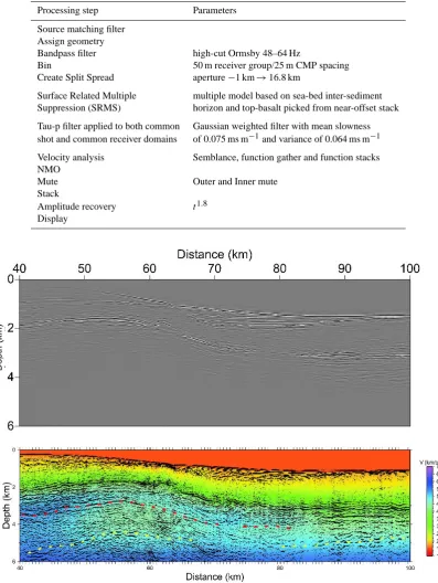
Table 1. Processing steps applied to data.

Processing step Parameters

Source matching filter Assign geometry

Bandpass filter high-cut Ormsby 48–64 Hz

Bin 50 m receiver group/25 m CMP spacing

Create Split Spread aperture−1 km→16.8 km

Surface Related Multiple multiple model based on sea-bed inter-sediment Suppression (SRMS) horizon and top-basalt picked from near-offset stack

Tau-p filter applied to both common Gaussian weighted filter with mean slowness shot and common receiver domains of 0.075 ms m−1and variance of 0.064 ms m−1

Velocity analysis Semblance, function gather and function stacks NMO

Mute Outer and Inner mute

Stack

Amplitude recovery t1.8 Display

I. Flecha et al.: Some improvements in subbasalt imaging using pre-stack depth migration 7

Figure 5.Top: stacked section from the FLO-96 survey. The top of basalt is clearly delineated. At the beginning of the profile (NW) basalt is shallower (around 1.8 s) becoming deeper from kilometer 60 to kilometer 75 where it remains practically flat around 3 s until the end of the profile (SE). No coherent subbasalt events can be identified. Bottom: Pre-stack depth migration of the same data set. The coloured background stands for the velocity model obtained by means of seismic tomography (Trinks et al., 2005). Dashed lines stand for interpreted base of basalt (red) and top of basement (yellow).

The code was then used with real data from the FLO-96 sur-vey. This processing showed that pre-stack depth migration improved the image obtained beneath the top of the basalt layer In the final image, the base of the basalt was inferred in some parts of the model and subbasalt events were

recov-ered. The results indicate that all offsets are required to

pro-duce a high frequency pre-stack depth migration image. The migrated section is highly dependent on the velocity model, therefore, using an accurate tomographic model is mandatory to obtain a reliable result.

Acknowledgements. Funding for this research was provided by SINDRI (Quantitative evaluation of the existing technologies for imaging within basalt-covered areas from the Faroes region), the Spanish Ministry of Science and Technology (Ref: CGL2004-04623/BTE) and Generalitat de Catalunya (Ref: 2005SGR00874). Part of this work was developed during a one month stay in Orsay

financed by Universit´e Paris-Sud. We are grateful to Immo Trinks for training in the use of the TTT code.

References

Fliedner, M. M. and White, R. S.: Sub-basalt imaging the Faeroe-Shetland Basin with large-offset data., First Break, 19, 247–252, 2001.

Fliedner, M. M. and White, R. S.: Depth imaging of basalt flows in the Faeroe-Shetland Basin., Geophys. J. Int., 152, 353–371, 2003.

Forel, D., Benz, T., and Pennington, W. D.: Seismic Data Process-ing with Seismic Un*x, Society of Exploration Geophysicists, 2005.

Fruehn, J., Fliedner, M. M., and White, R. S.: Integrated wide-angle and near-vertical subbasalt study using large-aperture seis-mic data from the Faroe-Shetland region, Geophysics, 66, 1340– 1348, 2001.

www.jn.net Journalname

Fig. 5. Top: stacked section from the FLO-96 survey. The top of basalt is clearly delineated. At the beginning of the profile (NW) basalt is shallower (around 1.8 s) becoming deeper from kilometer 60 to kilometer 75 where it remains practically flat around 3 s until the end of the profile (SE). No coherent subbasalt events can be identified. Bottom: pre-stack depth migration of the same data set. The coloured background stands for the velocity model obtained by means of seismic tomography (Trinks et al., 2005). Dashed lines stand for interpreted base of basalt (red) and top of basement (yellow).

(6)

6 I. Flecha et al.: Some improvements in subbasalt imaging using pre-stack depth migration interpreted as the base-basalt reflection and the top-basement

reflection (Fig. 4). In the last part of the profile, the top-basalt reflection could be identified while the basalt refraction com-pletely disappeared. This is due to the thinning of the basalt layer to the SE. Also in this part, some hyperbolic events were identified in the data out of the water-wave cone, but, due to the lack of lateral continuity (events only appeared for four or five shots), these events were interpreted as sills or laminar instrusions rather than a laterally continous geo-logical discontinuity. Inverting basalt refractions, top-basalt reflections, base-basalt reflections and basement reflections, a velocity model was obtained down to the top of the base-ment (coloured background in Fig. 5 bottom). The veloc-ity model was obtained using the tomographic algorithm by Trinks et al. (2005). This algorithm is able to use diving as well as reflected waves. Therefore it recovers the velocity distribution and the topography of the reflecting structures. In this study, the reflected phases were use to increase the resolution of the velocity model. The pre-stack migration al-gorithm only required the distribution of velocities to gener-ate the depth migrgener-ated image. The reflecting interfaces con-strained by the tomographic algorithm were not used. The image produced correlates very closely with the interfaces constrained by the inversion algorithm.

The sedimentary cover features velocities ranging from around 2 km s−1 at the sea bottom to 3.5 km s−1at the top of the basalt layer. A high velocity layer (4.5–5 km s−1) can be identified with a decreasing thickness from 1.5 km at 40 km to 0.5 km at 100 km. The inverted model suggests that there maybe a lower velocity layer under the basalts. Nev-ertheless, few events were identified from under the basalt layer, suggesting velocities in this area are less constrained than in other parts of the model. The lack of events within the basement made it impossible to extend the tomographic model beyond 6 km depth. The new pre-stack depth migra-tion scheme was used to obtain a new image using the veloc-ity determined by the tomographic inversion (Fig. 5 bottom). This method provided an improved display under the upper basalt interface where prominent events correlate with major velocity discontinuities along the whole model. The top of the basalt is clearly delineated. The base of this layer can be estimated in some parts of the model, especially along the first 30 km. In addition, some reflectors exist between 4 and 5 km depth which may correspond to the top of the basement. The determination of the base of the basalt layers is a key issue for exploration perspectives. Sedimentary layers can be located between the basalt intrusive and the basement. The importance of imaging these hidden sedimentary structures to gauge potential petroleum resources becomes clear.

Some authors have proposed an alternative scheme for mi-grating long offset reflection data (Fruehn et al., 2001; Flied-ner and White, 2001, 2003; White et al., 2003). Their scheme uses only selected signal out of the water-wave cone Follow-ing this strategy a low frequency image was produced be-cause only long offset phases were included. In the present

study, all the data in every shotgather were used in the pro-cess, obtaining a more detailed image because high frequen-cies were also included in the migration. Migrating selected parts of the shotgathers causes final image to be highly de-pendent on a subjective interpretation undertaken prior to the migration. This interpretation was considered when inverting traveltimes. Migrating the whole data set has the advantge of obtaining a migrated section free of a priori interpretations. Moreover, in regions where intra-basalt and subbasalt events are weak, the reflectors are more clearly displayed using all the data as shown in the last part of the profile.

5 Conclusions

Pre-stack depth migration provided improvement in sub-basalt imaging. The code developed to implement this tech-nique takes advantage of a finitte difference algorithm that can handle sharp velocity contrasts and velocity inversions avoiding shadow zones in the traveltime tables. Synthetic simulations using a realistic model showed a good perfor-mance of the code and good recovery of the original model. The code was then used with real data from the FLO-96 sur-vey. This processing showed that pre-stack depth migration improved the image obtained beneath the top of the basalt layer. In the final image, the base of the basalt was inferred in some parts of the model and subbasalt events were recov-ered. The results indicate that all offsets are required to pro-duce a high frequency pre-stack depth migration image. The migrated section is highly dependent on the velocity model, therefore, using an accurate tomographic model is mandatory to obtain a reliable result.

Acknowledgements. Funding for this research was provided by

SINDRI (Quantitative evaluation of the existing technologies for imaging within basalt-covered areas from the Faroes region), the Spanish Ministry of Science and Technology (Ref: CGL2004-04623/BTE) and Generalitat de Catalunya (Ref: 2005SGR00874). Part of this work was developed during a one month stay in Orsay financed by Universit´e Paris-Sud. We are grateful to Immo Trinks for training in the use of the TTT code.

Edited by: T. Iwasaki

References

Fliedner, M. M. and White, R. S.: Sub-basalt imaging the Faeroe-Shetland Basin with large-offset data, First Break, 19, 247–252, 2001.

Fliedner, M. M. and White, R. S.: Depth imaging of basalt flows in the Faeroe-Shetland Basin., Geophys. J. Int., 152, 353–371, 2003.

Forel, D., Benz, T., and Pennington, W. D.: Seismic Data Process-ing with Seismic Un*x, Society of Exploration Geophysicists, 2005.

Fruehn, J., Fliedner, M. M., and White, R. S.: Integrated wide-angle and near-vertical subbasalt study using large-aperture seismic

(7)

data from the Faroe-Shetland region, Geophysics, 66, 1340– 1348, 2001.

Hole, J. A. and Zelt, B. C.: Three-dimensional finite-difference re-flection travel times, Geophys. J. Int., 121, 427–434, 1995. Hughes, S., Barton, P. J., and Harrison, D.: Exploration in the

Shetland-Faeroe Basin using densely spaced arrays of ocean-bottom seismometers., Geophysics, 63, 490–501, 1998. Jones, I., Bloor, R. I., Biondi, B. L., and Etgen, J. T.: Prestack Depth

Migration and Velocit Model Building, Society of Exploration Geophysics, Geophysics reprint series, 25, 2008.

Maresh, J. and White, R. S.: Seeing through a glass, darkly: strate-gies for imaging through basalt, First Break, 23, 27–33, 2005. Martini, F. and Bean, C. J.: Interface scattering versus body

scatter-ing in subbasalt imagscatter-ing and application of prestack wave equa-tion datuming, Geophysics, 67, 1593–1601, 2002.

Noe-Nygaard, A. and Rasmussen, J.: Petrology of a 3000 metre sequence of basaltic lavas in the Faroe Islands, Lithos, 1, 286– 304, 1968.

Raum, T., Mjelde, R., Berge, A. M., Paulsen, J. T., Digranes, P., Shimamura, H., Shiobara, H., Kodaira, S., Larsen, V. B., Fred-sted, R., Harrison, D. J., and Johnson, M.: Sub-basalt structures east of the Faroe Islands revealed from wide-angle seismic and gravity data, Petrol. Geosci., 11, 291–308, 2005.

Richardson, K. R., White, R. S., England, R. W., and Fruehn, J.: Crustal structure east of the Faroe Islands: mapping sub-basalt sediments using wide-angle seismic data, Petrol. Geosci., 5, 161– 172, 1999.

Smallwood, J. R., Towns, M. J., and White, R. S.: Thew structure of the Faeroe-Shetland Trough from integrated deep seismic and potential field modelling, J. Geol. Soc., 158, 409–412, 2001. Sørensen, A. B.: Cenozoic basin development and stratigraphy of

the Faroes area, Petrol. Geosci., 9, 189–207, 2003.

Trinks, I., Singh, S. C., Chapman, C. H., Barton, P. J., Bosch, M., and Cherrett, A.: Adaptative traveltime tomography of densely sampled seismic data, Geophys. J. Int., 160, 925–938, 2005. White, R. S., Fruehn, J., Richardson, K. R., Cullen, E., Kirk, W.,

Smallwood, J. R., and Latkiewicz, C.: Faroes Large Aperture Research Experiment (FLARE): imaging through basalt, Geo-logical Society, 1243–1252, 1999.

White, R. S., Smallwood, J. R., Fliedner, M. M., Boslaugh, B., Maresh, J., and Fruehn, J.: Imaging and regional distribution of basalt flows in the Faroe-Shetland Basin., Geophys. Prosp., 51, 215–231, 2003.

Yilmaz, O.: Seismic data processing, Society of Exploration Geo-physicists, Tulsa, 1987.

Zelt, C. A. and Smith, R. B.: Seismic traveltime inversion for 2-D crustal velocity structure, Geophys. J. Int., 108, 16–34, 1992.