Correction of static pressure on a research aircraft in accelerated flight using differential pressure measurements

Correspondence to: A. R. Rodi (rodi@uwyo.edu)

Received: 9 April 2012 – Published in Atmos. Meas. Tech. Discuss.: 21 May 2012

Revised: 14 September 2012 – Accepted: 17 September 2012 – Published: 1 November 2012

Abstract. A method is described that estimates the error in the static pressure measurement on an aircraft from differen-tial pressure measurements on the hemispherical surface of a Rosemount model 858AJ air velocity probe mounted on a boom ahead of the aircraft. The theoretical predictions for how the pressure should vary over the surface of the hemi-sphere, involving an unknown sensitivity parameter, leads to a set of equations that can be solved for the unknowns – angle of attack, angle of sideslip, dynamic pressure and the error in static pressure – if the sensitivity factor can be determined. The sensitivity factor was determined on the University of Wyoming King Air research aircraft by comparisons with the error measured with a carefully designed sonde towed on connecting tubing behind the aircraft – a trailing cone – and the result was shown to have a precision of about±10 Pa over a wide range of conditions, including various altitudes, power settings, and gear and flap extensions. Under acceler-ated flight conditions, geometric altitude data from a com-bined Global Navigation Satellite System (GNSS) and iner-tial measurement unit (IMU) system are used to estimate ac-celeration effects on the error, and the algorithm is shown to predict corrections to a precision of better than±20 Pa under those conditions. Some limiting factors affecting the preci-sion of static pressure measurement on a research aircraft are discussed.

1 Introduction

Static pressure measurement on an aircraft is inherently prob-lematic because the pressure changes as the air accelerates around the wings and fuselage, as predicted by the Bernoulli equation. It is difficult to find a location on the aircraft to measure the true undisturbed pressure,P∞, i.e., the pressure

at a distance far from the flow-disturbing effects. On the air-craft, static pressurePs is measured at a set of ports where

the aircraft designers have determined that the error, re-ferred to as the static defect or position error, is minimal. In addition to causing errors in pressure-derived aircraft alti-tude, the static defect also leads directly to errors in airspeed and other measurements that need dynamic corrections, such as temperature, for example. In the pitot tube technique of airspeed measurement (Doebelin, 1990), dynamic pressure qc=PT−Ps'1/2ρU2is sensed, wherePTis the total

pres-sure,ρthe air density, andUthe airspeed. On the University of Wyoming King Air (UWKA) research aircraft, static pres-sure errors can be as large as 2 % ofqc at research aircraft speeds (∼100 m s−1), and this error transfers directly to an error of 1 % (1 m s−1) in airspeed. These errors directly affect estimates of atmospheric air motions which are sensed using the “drift method” in which the three-dimensional airspeed and ground velocity vectors are subtracted.

Static pressure becomes more problematic when aircraft are used in the study of pressure fields in baroclinic zones or cloud systems. Bellamy (1945) introduced airborne de-termination of D-value, the difference between the radar-determined geometric altitude and the pressure altitude from static pressure, using the standard atmosphere assumption. Shapiro and Kennedy (1981) and Brown et al. (1981) ap-plied this to the determination of jet stream geostrophic and ageostrophic winds. This pressure gradient approach has also been used for studies of low-level jets (Rodi and Parish, 1988; Parish et al., 1988; Parish, 2000). LeMone and Tar-leton (1986) and LeMone et al. (1988) used altitude de-rived from accelerometer measurements instead of radar al-titude in perturbation pressure studies around clouds sug-gesting that accuracies of 20 Pa can be obtained, but only with substantial empirical corrections and carefully flown legs. More recently, Parish et al. (2007) and Parish and Leon (2012) demonstrated that Global Navigation Satellite System (GNSS, hereafter referred to as global positioning system – GPS) data can resolve both pressure gradients and perturba-tions associated with mesoscale and cloud-scale systems.

In this study, we develop and test a method for estimating static defect using differential pressure measurements on the hemispherical leading surface of a Rosemount model 858AJ (hereafter R858) air velocity probe. The theoretical predic-tions for how the pressure should vary (presented in the Ap-pendix) lead to a set of equations that can be used to solve the static pressure error in addition to the attack angle, sideslip angle and dynamic pressure. We first use trailing sonde data to determine the probe sensitivity factor, and then compare resulting error estimates with accurate altitude measurements from a GPS-aided inertial measurement unit (IMU), allowing for an independent check of the precision of the algorithm and an examination of the effects of aircraft acceleration.

2 Retrieval of static pressure error from differential pressure measurements

B¨ogel and Baumann (1991) describe a method of analysis of R858 measurements during pilot-induced maneuvers to esti-mate static pressure errors. Crawford and Dobosy (1992) de-scribe the Best Aircraft Turbulence (BAT) differential pres-sure flow-angle probe which addresses the static prespres-sure problem by averaging pressure on several ports. Here, we develop a method to predict the static pressure error directly by using pressure measurements from the R858 air veloc-ity probe which, on the UWKA, is mounted at the tip of a boom, as shown in Fig. 1. The probe is a hemisphere-cylinder configuration in which a hemispherical surface is at the end of a 2.5 cm diameter, 12.5 cm long cylindrical section. Pressure measurements on ports in a hemispheri-cal surface are used for airspeed and flow angle determina-tion (Brown et al., 1983). There are 5 ports: one central port which approximates total pressure, two ports separated by

Fig. 1. UWKA showing nose boom location.

±45◦ from the central axis in the aircraft horizontal plane for sideslip angle determination, and two ports separated by

±45◦in the aircraft vertical plane for attack angle determi-nation.

In the UWKA system, four differential pressure measure-ments are made, allowing the static error to be estimated. The method and specific equations used in the UWKA R858 con-figuration are presented in the Appendix. The attack angleα, for example, can be estimated as described in the manufac-turer’s technical note (Rosemount, 1976) using

α'Pα1−Pα2

Kqc

(1) where the numerator is the differential pressure between the two attack angle ports. The sensitivity coefficient, assuming potential flow (using a sensitivity factor, as defined in the Appendix,f =9/4) for small angles, isK∼=2f (π/180)=

0.0785 deg−1. Brown et al. (1983) investigatedKusing data from flight maneuvers for the R858 on the noseboom on the NCAR Sabreliner. They found that for NMach<0.5, K=

0.068 deg−1(f =1.95), 13 % lower than the value recom-mended in Rosemount (1976). This determination ofKwas not exact nor without ambiguities, however. The Brown et al. (1983) method substituted precise IMU-measured pitch an-gle for attack anan-gle, which is valid during periods of straight and level flight assuming zero vertical wind and aircraft ver-tical velocity. Using pitch in this manner, the upwash effect (Crawford et al., 1996) of the fuselage, wings, and possibly the R858 itself is incorporated into the value ofK. The sense of upwash effect is to make the local attack angle larger than the pitch angle, causingKto be overestimated compared to the local value ofKwithout the upwash effect. Brown et al. (1983) apparently also used1P1forq without static defect

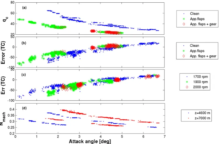
Fig. 2. Scatter plots (10 Hz data) as functions of attack angle [deg] for various flight configurations and altitudes as indicated in legends: (a) dynamic pressureqc[hPa], (b) and (c) static pressure error [Pa] determined by TC, and (d) Mach number.

estimated directly so that the upwash effect is not accounted for so that the flow angles that result are relative to the hemi-spherical surface, andqis corrected for flow angle.

We now show that the static pressure error can be deter-mined from the differential pressure measurements, assum-ing that sensitivity factorf can be determined. The theoret-ical predictions of the four differential measurements from the Appendix (Eq. A11) are:

1P1=P1−Ps,m=q[1−(f−1)(tan2α+tan2β)/

(1+tan2α+tan2β)] −Perr

1Pα=P4−P5=2f qtanα/(1+tan2α+tan2β)

1Pβ =P2−P3=2f qtanβ/(1+tan2α+tan2β)

1PR=P1−P2=f q(1−2 tanβ−tan2β)/

2(1+tan2α+tan2β)

(2)

where here we have replacedP∞in Eq. (A11) with the

mea-sured static pressurePs,mless the unknown errorPerr, and the

remaining unknowns are the attack angleα, sideslip angleβ, dynamic pressureq, and the probe sensitivityf.

We note that we are solving for the error, using the expres-sion for1P1in Eq. (2) rearranged as

Perr=q[1−(f−1)(tan2α+tan2β)/

(1+tan2α+tan2β)] −1P1

. (3)

We show in the Appendix thatαandβ can be found with-out a priori knowledge off. Thus,Perris the departure of

1P1 from q after the attack and sideslip angle correction.

The strategy is to develop an estimatef using the trailing

Fig. 3. Scatter plots (10 Hz data) of probe sensitivity factorf, cal-culated from the solution of Eq. (2), versus1Pα [hPa](top panel), and Mach number (bottom panel) for various flight configurations and altitudes, as indicated in legend.

cone test data, described in the next section, and then es-timate Perr as one of the unknowns from the four pressure

Fig. 4. Pressure error[Pa]predicted from differential pressure algo-rithm vs. error measured with TC for various flight configurations, altitudes and propellor speeds, as indicated in legends (10 Hz data). 1:1 lines are shown.

3 Trailing cone test data

Ikhtiari and Marth (1964) and Mabry and Brumby (1968) de-scribe an aircraft pressure calibration system in which a static pressure probe, connected to the aircraft by tubing, is towed at some distance behind and below the aircraft, away from the disturbing influence of the aircraft. The towed sonde is stabilized in flight by means of a carefully engineered cone – thus the term “trailing cone” (hereafter called TC ) – that creates drag for stabilization of static pressure ports which are distributed around the circumference of a straight piece of tubing behind the cone. Brown (1988) described the tech-nique in detail, and demonstrated for the NCAR Sabreliner that the largest expected error in the pressure measurement is±39 Pa after application of corrections based upon the TC data. The distance that the TC is extended is chosen to be long enough to minimize pressure fluctuations in the air-craft’s wake. However, accelerations cause errors. For ex-ample, with a 19 m tubing length (the length used for the UWKA), a 0.1 g acceleration will result in a 15 Pa effect. Consequently, we limit data collection to steady, straight flight legs.

A UWKA test flight using the Douglas model 501 TC was conducted on 27 October 2005. Data were collected in sev-eral configurations: (1) with the aircraft in “clean” configu-ration (landing gear raised, flaps retracted), (2) in segments with gear lowered, (3) with gear lowered and flaps extended in approach mode, and (4) at different power settings and al-titudes. Several measured variables are shown in Fig. 2 as a function of aircraft attack angle, using data filtered at 5 Hz and output at 10 Hz. The lack of a single relationship for all configurations among dynamic pressure, pressure error, and NMachis evident. This is the main obstacle to simple

correc-tions as a function of one variable such as dynamic pressure or attack angle.

Fig. 5. Distribution of residual error (DP algorithm prediction minus

TC measurement)[Pa](10 Hz data).

4 Empirical determination of f from trailing cone data

We first solved Eq. (2) for the unknown values off,α,β, andqc using TC flight measurements ofPerrand

differen-tial pressures1P1,1Pα,1Pβ, and1PR. The resulting f-values are plotted in Fig. 3, and show increases with1Pα, and decreases withNMach. We then used a non-linear

regres-sion procedure to obtain the empirical estimate offthat best predicts the TC-determinedPerr. The best fit was found by

trial and error selection of variables to be:

f =c0+c1NMach+c2NMach2 +c31Pα (4) where the constants were found to be c0=1.700, c1=

−0.1569, c2=0.06633 and c3= +0.001254, and where

1Pα is in units of hPa. A discussion of the physical basis for these relationships will be presented later.

The resulting predictions of pressure error are compared with TC measurements in Fig. 4 at various steady flight con-figurations and power settings. The distribution of the resid-ual errors is shown in Fig. 5 to have a precision±10 Pa in all configurations (σ=8 Pa).

There is additional evidence for the variability of f. Brown et al. (1983) and Rosemount (1976) provide ex-perimental evidence for f decreasing withNMach,

consis-tent with the present results. Traub and Rediniotis (2003) (TR03) present an analytical prediction of surface pressures for a hemisphere-cylinder configuration similar to the R858, and wind tunnel results at Reynolds numbers about a fac-tor of two higher than UWKA flight (NRe≈1.5×104). The TR03 theoretical formulation, confirmed by their wind tun-nel results, predicts sensitivity to be f=2.07 at zero in-cidence angle, and also their data show that the sensitivity varies with incidence angle.

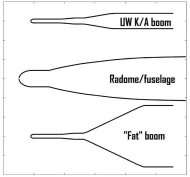
Fig. 6. Models of aircraft and boom configurations (see text).

compressible flow equations (FIDAP, Fluid Dynamics Inter-national, Inc.). An axisymmetric, compressible model at zero attack angle was used and showed thatf is different for var-ious mounting configurations, and changes with speed. So-lutions were found for NMach equivalent to speeds of 50–

180 m s−1. Four configurations were modeled as shown in Fig. 6 (not to scale): (1) a sphere (not shown); (2) the R858 probe mounted on the end of the UWKA nose boom, which is 0.2 m in diameter; (3) the spherical radome (nose radar cov-ering) as on the former National Science Foundation (NSF) King Air aircraft (N308D); and (4) the R858 mounted on a nose boom four times the diameter of the actual UWKA nose boom. Pressure distributions on the spherical surface were fit using the sin2 relationship (A1), and the result-ingf for eachNMach plotted in Fig. 7a. For the sphere, f

varies from 1.9–2.1. Adding the nose boom behind the R858 hemisphere-cylinder decreasesf to about 1.9. Increasing the boom diameter to 0.8 m lowersf to about 1.5. These results suggest that there is no unique value off for all mounting configurations of the R858. Indeed, the fuselage of the air-craft itself presents a formidable aerodynamic barrier to the probe, which is likely to contribute to the actualf variability in addition to a particular mounting configuration.

To explore further the behavior of f, we constructed a physical model of the R858 with extra pressure ports drilled so that adequacy of the sin2relationship between angle and pressure could be determined by direct measurement along with determination off. The test was conducted in the Uni-versity of Wyoming Low Speed Wind Tunnel, which has a test section of 0.6×0.6×0.9 m. The model was constructed 75 % larger than the actual probe so that the Reynolds num-ber at the test speed of 50 m s−1 would be approximately that of the actual (0.0254 m diameter) probe at 90 m s−1, the typical flight speed for the UWKA. Data were digi-tized with a personal-computer-based data logging system at 10 Hz after analog filtering with cutoff frequency of 2 Hz.

Fig. 7. Estimation of sensitivity factorf from (a) modeling and

(b) values from Brown et al. (1983), (Rosemount, 1976), and

so-lution to Eq. (A11) for UW King Air flight data. The point labeled “T” represents the value from determined from the wind tunnel tests of the R858 model.

The analysis then was performed on one minute averages of pressures at each port. Additional measurements made with a standard pitot tube placed upwind from the test body to ensure that the tunnel speed did not change during runs at each attack angle. In Fig. 7b, the sensitivity off toNmach

from Brown et al. (1983) and (Rosemount, 1976) are shown, along withf determined from the wind tunnel tests (point labeled as “T”), and the solution of Eq. (2) with actual King Air flight data.

5 Measured pressure compared to pressure derived from GPS altitude

While the 2005 TC test flight varied attack angle with air-speed and altitude, sideslip angles were intentionally kept near zero to prevent lateral acceleration. In this section, the efficacy of the estimates ofPerrin an accelerating flight

envi-ronment using the differential pressure solution described in the previous section will be examined.

Differential global positioning system (dGPS) techniques use data from one or more stationary reference or base GPS stations which have precisely determined location to refine position estimates for the receiver on the aircraft. dGPS processing techniques using dual-frequency (L1/L2) carrier phase data can eliminate errors caused by ionospheric and tropospheric delays entirely, resulting in position esti-mates with accuracy of centimeters under optimal conditions (Parish et al., 2007).

Fig. 8. Time series of (a) height difference (geometric-pressure)

[m], (b) attack angle [deg], (c) sideslip angle [deg], and (d) pres-sure deviation from lever arm correction [Pa]. Time series is the concatenation of four 500 s segments, the first two flown at 4600 m, the second two at 7000 m.

(Trimble/Applanix model AV410). The IMU data, recorded at 200 Hz, were corrected in post-processing using Trim-ble/Applanix POSPac software which implements a tightly-coupled Kalman filter between the IMU and dGPS data. The processing fully removed all L1/L2 cycle ambiguities in a fixed, narrow lane processing mode. Position accuracy estimated by the manufacturer is shown in Table 1. The re-sulting 200 Hz values of aircraft position and attitude were low-pass filtered with a cutoff frequency of 10 Hz and then decimated to 20 Hz for the present analysis. Also, accurate time synchronization of the IMU and pressure measurements was assured by GPS time stamping of all data.

Static pressure was measured with the Rosemount 1501 High Accuracy Digital Sensing Module (HADS) which has static accuracy of 20 Pa and a digital resolution of 1.8 Pa. The accuracy includes effects of non-linearity, repeatability, temperature (−51 to 80◦C) and calibration. Worst case error from transducer acceleration is specified to be 20 Pa under acceleration of 6 g; the maximum acceleration in these tests was±1 g. We estimate the maximum dynamic errors in the connecting tubing to be 10 Pa for longitudinal accelerations (here 0.1 g, 10 m tubing length) and lateral (1 g, 1 m tubing length) accelerations of the air column.

Flight data were collected on 16 September 2011 during pilot-induced maneuvers inducing variations in attack and sideslip angles. Periods of turns were not considered in the analysis. The aircraft was flown at nominally constant pres-sure with deviations corrected hydrostatically to that prespres-sure using the method described by Parish et al. (2007). Pressure-derived altitude changes were determined from integration of the hydrostatic equation:

Fig. 9. Scatter plots of: (top panel) attack angle [deg] vs. vertical

acceleration [m s−2]; and (bottom panel) sideslip angle [deg] vs. lateral acceleration [m s−2].

Table 1. Trimble/Applanix airborne positioning system

perfor-mance specifications.

AV410 Absolute Accuracy Post-processed

Position (m) 0.05–0.30

Velocity (m s−1) 0.005 Roll and Pitch (deg) 0.008 True Heading (deg) 0.025

AV410 Relative Accuracy

Noise (deg h−0.5) <0.1 Drift (deg h−1)∗ 0.5

∗_{Attitude will drift at this rate up to the maximum absolute}

accuracy.

z−z0= −

P Z

P0 RdryTv

g d lnP (5)

wherez0is a direct measurement of geometric altitude from

the IMU/dGPS system at pressureP0and virtual temperature

Tv. Data were collected at two altitudes – nominally 4600 and

7000 m m.s.l. Other relevant measurements include in-house developed reverse flow temperature (accuracy of 0.5 K, reso-lution of 0.006 K), and Edgetech Model 137 dew point tem-perature (accuracy of 1 K, resolution 0.006 K).

A bias is introduced if an atmospheric horizontal pressure gradient exists, or when pressure is falling, along the flight track since constant geometric height is no longer constant pressure. To minimize this effect, the time series is broken up into 500 s segments and reinitialized withz0from the highly

Fig. 10. Concatenated time series as in Fig. 8: (top panel) aircraft

height [m] (m.s.l.); and (bottom panel) pressure error determined from IMU/dGPS before correction [Pa].

The Laramie Valley was under the influence of high pressure, clear sky, and weak pressure gradient during the analysis pe-riod, which minimized the pressure change effect.

Computing geometric altitude from measured static pres-sure also involved carefully considering the relative distance vectors of the inertial measurement unit (IMU), GPS an-tenna, R858, and the static pressure locations. These vectors were accurately determined with accuracy<5 cm using pre-cise surveying techniques. The resulting “lever arm” fluctua-tions were less than 8 Pa during the sideslip and 15 Pa during the attack angle changes, as shown in Fig. 8d.

The angle changes with periods of about 10 s, as shown in Fig. 8b, result in correlated vertical accelerations as shown in Fig. 9. The attack angle was limited to−2 to−12◦, resulting in±1 g changes, helping to avoid excessively large altitude excursions. The sideslip angles (Fig. 8c) were restricted to

±8◦, limiting lateral accelerations to±0.20 g lateral acceler-ations for crew comfort and also safety consideracceler-ations. Typi-cal values during research flights are less than±0.5 g,±1 g in strong turbulence, and only rarely experiencing the±2 g lim-itation set under U.S. Federal Aviation Administration Part 91 certification. In our experience, instantaneous attack an-gle values in severe turbulence have been noted to reach 20◦ while the aircraft is still within the g-loading limits, but this is rare. The resulting static pressure errors from the maneu-vers are shown in Fig. 10. The pressure-geometric altitude errors for sideslipping have a range of about 50 Pa and for attack angle changes a range of about 300 Pa

The errors before and after correction are shown in Fig. 11 for the attack and sideslip changes, with the distribution of errors before and after correction shown in Fig. 12. After cor-rection, the biases in during the attack and sideslip changes were−14 and+10 Pa, respectively, with standard deviations of 16 and 11 Pa, respectively.

Fig. 11. Time series of errors [Pa] from Fig. 10: (a) and (b) are before and after correction, respectively, for attack changes; (c) and

(d) before and after correction, respectively, for sideslip changes.

Fig. 12. Distribution of errors [Pa] for data shown in Fig. 11 before

correction (red) and residual after correction (blue) for (a) attack angle changes; and (b) sideslip angle changes.

6 Frequency response

Fig. 13. Power spectral density [variance/frequency unit] versus

fre-quency [Hz] for period of attack angle change at 7000 m altitude. Left axis: corrected static pressure [Pa], and pressure correction [Pa]. Right axis: vertical wind component [m s−1] and inertial sub-range−5/3 slope.

Fig. 14. Power spectral density as in Fig. 13 for period of sideslip

angle changes at 7000 m altitude.

of about 15 Pa, which is above the whitening effect of the digitization noise (2 Pa). The sharp disturbances at 30–40 Hz in Fig. 14 (sideslip periods) are probably due to the 4-bladed propellers, which operate normally at about 1700 rpm.

7 Summary and discussion

An algorithm was developed to estimate static pressure errors in steady flight using R858 differential pressure measure-ments, and tested with trailing cone data from a University of Wyoming King Air flight in 2005. After calibratingf us-ing the TC flight data, it was shown that the effects of speed, altitude and flight configuration (landing gear, flap extension) can be predicted toσ =8 Pa in steady flight. To capture the

effects of acceleration, flight maneuvers were conducted and geometric altitude from a GPS-aided inertial measurement data were used to predict the pressure error. These results suggest that pressure errors can be determined with a preci-sion of±20 Pa during such maneuvers. It should be empha-sized that the precision, not the absolute accuracy, of these estimates is addressed in this paper. The absolute accuracy of the error estimates using this method depend on this em-pirical determination off as well as other factors addressed in the present work.

Our attempts to use statistical regression analysis alone to relate the observed pressure error to flight data (NMach,qc, inertial acceleration) have not been successful. The differen-tial pressure method, however, has the advantage of being a solution based upon the R858 equations, as presented in the Appendix. The main weakness is that determination of the probe sensitivityf requires an independent means of its determination. In the present study, we used the TC measure-ments to calibratef.

There are several sources of error which may be a factor in the interpretation. The effect of acceleration of the air in the connecting tubing, which we estimate to be smaller than 10 Pa, is indistinguishable from the aerodynamic cause of the static defect at the sensing ports. Nonetheless, the R858 pres-sure imbalance approach should capture the connecting tub-ing effect. The other factor is the error introduced by uncer-tainty in height differences between the static pressure ports at the rear of the fuselage, IMU and GPS antenna locations, and R858 probe tip. Figure 8d shows this effect is<−15 Pa. Our flow modeling suggests that the relatively low esti-mates off from the algorithm (f∼=1.7) may be reasonable sincef was found to decrease as the structure behind the R858 hemisphere-cylinder gets larger (Fig. 7). These values are lower than TR03 (hemisphere-cylinder,f =2.07) which also suggest thatf varies with incidence angle. It would be useful to obtain independent confirmation of these estimates, for example, by using pitch angle as a surrogate forαat dif-fering airspeeds, as described by Brown et al. (1983). But that approach has limitations, as discussed in Sect. 2, especially since using pitch as an estimate ofαimplicitly incorporates the upwash effect (Crawford et al., 1996) into the sensitiv-ity. Further, using a separate pitot tube measurement for q would itself require the correction for static defect. The prob-lems extend to the horizontal with sidewash effects. Thus, we think that independently estimatingf, while desirable, is problematic at best and beyond the scope of this paper.

spherical 5-hole probe

The derivation of the relationships among the pressures on a 5-hole spherical probe surface and the attack and sideslip flow angles follows. Hale and Norrie (1967), Brown et al. (1983), and Nacass (1992) analyzed the differential pressures between ports in terms of the well-known pressure distribu-tion on a sphere in terms of the coefficient of pressureCp:

Cp=

P−P∞

q =1−fsin

2_{φ (A1)}

whereP is the pressure at solid angleφfrom the stagnation point,P∞is the pressure in the free stream,q'1/2ρU2is

the dynamic pressure,ρ is the air density,U the speed, and f the sensitivity factor;f =9/4 for potential flow (Lamb, 1932).

A coordinate system is defined by unit vectors as follows:ˆi along the x-axis forward through the center port;jˆalong the y-axis to the right, andkˆlong the z-axis down in aircraft co-ordinates. The angleφin Eq. (A1) is the “great circle” angle between the stagnation point and point of pressure measure-ment at one of the five ports (Nacass, 1992). We define two more unit vectors in terms of their direction cosines from the probe axes: one,λˆ0, from the center of the probe hemisphere

through the stagnation point, and the other,λˆa, through the pressure port of interest. Thus,

ˆ

λ0= ˆicosθx0+ ˆjcosθy0+ ˆkcosθz0

ˆ

λa= ˆicosθxa+ ˆjcosθya+ ˆkcosθza

(A2)

and the direction cosines for each vector are constrained by the identity

cos2θx+cos2θy+cos2θz=1. (A3) Angleφthen can be found from the definition of the cross product of two vectors

sinφ= | ˆλa× ˆλ0|/| ˆλa|| ˆλ0| (A4)

sin2φ1=1−cos2θx0

sin2φ2=(cosθx0cosθy2−cosθy0cosθx2)2+cos2θz0

sin2φ3=(cosθx0cosθy3−cosθy0cosθx3)2+cos2θz0 (A6)

sin2φ4=(cosθx0cosθz4−cosθz0cosθx4)2+cos2θy0

sin2φ5=(cosθx0cosθz5−cosθz0cosθx5)2+cos2θy0

,

where the first subscript on the direction cosines is the axis direction, and the second subscript is the port number or 0 being the stagnation point.

Four differential pressures are measured:P1−P∞which

approximately the impact pressureqcat small angles,P2−P3

in the plane of the probe horizontal axis defining the sideslip angleβ,P4−P5in the plane of the probe vertical axis

defin-ing the attack angle α, and P1−P2 which is also a

mea-sure of the impact presmea-sure, as suggested by Rosemount (1976) for their Model 858 5-hole probe. The center port then hasθxa=0◦, cosθxa=1, and the remaining ports are at θ=45◦_{, cosθ}

ya=cosθza=

√

2/2. Combining these angles and differential pressure definitions with Eq. (A6) applied to Eq. (A1) gives the following set of equations for the differ-ential pressures:

P1−P∞=q[1−f (1−cos2θx0)]

P2−P3=2qfcosθx0cosθy0

P4−P5=2qfcosθx0cosθz0

P1−P2=

1 2qf (cos

2_θ

x0−cos2θy0−2 cosθx0cosθy0)

.

(A7)

We now define the attack angle α and sideslip angle β as functions of the velocity components in terms of the direction cosines (Ux/U=cosθx0, etc.):

tanα= Uz

Ux

=Ucosθz0

Ucosθx0

=cosθz0

cosθx0

(A8)

tanβ=Uy

Ux

=Ucosθy0

Ucosθx0

=cosθy0

cosθx0

Note thatβ as defined here is not the standard definition of sideslip (ISO, 1985), but is the commonly used definition because of its natural relation toUyin the wind computation. Equations (A8) and (A9) can be solved for the direction cosines as

cosθx0=1/(1+tan2α+tan2β) 1/2

cosθy0=tanβ/(1+tan2α+tan2β) 1/2

cosθz0=tanα/(1+tan2α+tan2β) 1/2

.

(A10)

Equations (A7)–(A10) can be combined to give the final set of equations, assuming exact knowledge ofP∞:

1P1=P1−P∞=q[1−(f−1)(tan2α+tan2β)/

(1+tan2_α+tan2_β)]

1Pα=P4−P5=2f qtanα/(1+tan2α+tan2β)

1Pβ =P2−P3=2f qtanβ/(1+tan2α+tan2β)

1PR=P1−P2=f q(1−2 tanβ−tan2β)/

2(1+tan2α+tan2β).

(A11)

Equation (A11) can be solved either numerically or analyti-cally for the unknowns tanβ, tanα,qandf. The1Pα, 1Pβ, and1PR equations can be solved analytically tanβ, tanα without a priori knowledge of dynamic pressureq or sensi-tivity factorf. Those solutions are:

tanβ=(q2(1P_β2+21Pβ1PR+21PR2) −1Pβ−21PR)/1Pβ

tanα=(tanβ)1Pα/1Pβ.

(A12)

We note that the limiting relationship when1PB→0 is tanα= 1Pα

41PR

(A13) and

q=1P

2

α+81P11PR

81PR

. (A14)

Acknowledgements. This study was supported by NSF Cooper-ative Agreement AGS-0334908, and NSF Grant AGS-1034862. The authors would like to thank colleagues in the Department of Atmospheric Science at the University of Wyoming and the UWKA facility team for collection and processing of the data, and Prof. William Lindberg, UW Department of Mechanical Engineering, for assistance with the wind tunnel measurements and recording. We also would like to thank an anonymous reviewer for suggesting important improvements in the text, and also for noticing a typographical error in the equations in the Appendix.

Edited by: P. Herckes

References

Bellamy, J. C.: The use of pressure altitude and altimeter correc-tions in meteorology, J. Meteorol., 2, 1–79, doi:10.1175/1520-0469(1945)002<0001:TUOPAA>2.0.CO;2, 1945.

B¨ogel, W. and Baumann, R.: Test and calibration of the DLR Falcon wind measuring system by maneuvers, J. Atmos. Ocean. Tech., 8, 5–18, doi:10.1175/1520-0426(1991)008<0005:TACOTD>2.0.CO;2, 1991.

Brown, E. N.: Position Error Calibration of a Pressure Sur-vey Aircraft Using a Trailing Cone, Tech. Rep. NCAR/TN-313+STR, National Center for Atmospheric Research, Boulder, CO, doi:10.5065/D6X34VF1, 1988.

Brown, E. N., Shapiro, M. A., Kennedy, P. J., and Friehe, C. A.: The application of airborne radar altimetry to the measurement of height and slope of isobaric sur-faces, J. Appl. Meteorol., 20, 171–180, doi:10.1175/1520-0450(1981)020<1070:TAOARA>2.0.CO;2, 1981.

Brown, E. N., Friehe, C. A., and Lenschow, D. H.: The use of pressure fluctuations on the nose of an aircraft for mea-suring air motion, J. Clim. Appl. Meteorol., 22, 1070–1075, doi:10.1175/1520-0450(1983)022<0171:TUOPFO>2.0.CO;2, 1983.

Crawford, T. L. and Dobosy, R. J.: A sensitive fast-response probe to measure turbulence and heat-flux from any airplane, Bound.-Lay. Meteorol., 59, 257–278, doi:10.1007/BF00119816, 1992. Crawford, T. L., Dobosy, R. J., and Dumas, E. J.: Aircraft wind

measurement considering lift-induced upwash, Bound.-Lay. Me-teorol., 80, 79–94, doi:10.1007/BF00119012, 1996.

Doebelin, E. O.: Measurement systems: application and design, McGraw-Hill, New York, 4th Edn., ISBN: 978-0070173385, 1990.

Hale, M. R. and Norrie, D. H.: The analysis and calibration the five-hole spherical pitot, Tech. Rep. ASME Publication 67-WA/FE-24, Amer. Soc. Mech. Eng., New York, 1967.

Ikhtiari, P. A. and Marth, V. G.: Trailing cone static pressure mea-surement device, J. Aircraft, 1, 93–94, doi:10.2514/3.43563, 1964.

ISO: Flight dynamics, concepts and quantities Part 2: Motions of aircraft and the atmosphere relative to the earth, 2nd Edn., Ref. No. ISO 1151/2-1985(E), International Organization for Stan-dardization, Geneva, Switzerland, 1985.

Lamb, H.: Hydrodynamics, Dover Publications, New York, ISBN: 978-0486602561, 1932.

LeMone, M. A. and Tarleton, L. F.: The use of inertial altitude in the determination of the convective-scale pressure field over land, J. Atmos. Ocean. Tech., 3, 650–661, doi:10.1175/1520-0426(1986)003<0650:TUOIAI>2.0.CO;2, 1986.

LeMone, M. A., Tarleton, L. F., and Barnes, G. M.: Per-turbation pressure at the base of cumulus clouds in low shear, Mon. Weather Rev., 116, 2062–2068, doi:10.1175/1520-0493(1988)116<2062:PPATBO>2.0.CO;2, 1988.

Mabry, G. and Brumby, R.: DC-8 Airspeed Static Position Error Repeatability, Tech. Rep. Douglas Paper 5517, Douglas Aircraft Co., Unk., 1968.