Article
A Semi-Parametric Approach to the Oaxaca–Blinder
Decomposition with Continuous Group Variable
and Self-Selection
Fernando Rios-Avila
Levy Economics Institute, Bard College, Annandale-on-Hudson, NY 12504, USA; [email protected]
Received: 22 February 2019; Accepted: 18 June 2019; Published: 21 June 2019
Abstract:This paper presents an extension to the Oaxaca–Blinder decomposition with continuous groups using a semiparametric approach known as varying coefficients model. To account for potential self-selection into the continuum of groups, the use of inverse mills ratios is expanded upon following the literature on endogenous selection. The flexibility of this methodology may allow detecting heterogeneity when analyzing endogenous dose treatments effects, as well as correcting for endogeneity when analyzing the heterogeneous partial effects across the continuous group variable. For illustration, the methodology is used to revisit the impact of body weight on wages, using body mass index (BMI) as the continuum of groups, finding evidence that body weight has a negative, but decreasing impact on wages for both white men and women.
Keywords: Oaxaca–Blinder Decomposition; heckman selection; semi-parametric; endogeneity; kernel; non-linear; BMI; Body weight; wages differentials
JEL Classification:C14; I19; J31; J71
1. Introduction
Since the seminal papers fromBlinder(1973) andOaxaca(1973), many studies have used what is known as the Oaxaca–Blinder (OB) decomposition for analyzing outcomes differences between two well defined groups. Such differences are characterized as functions of differences in characteristics (composition effect) and differences in coefficients associated with those characteristics (wagestructure effect). Subsequent research provided refinements that extended the OB decomposition analysis to non-linear functions, distributional statistics other than the mean, as well as strategies to identify the model when some of the underlying assumptions do not hold (seeFortin et al.(2011) for a review of other methodological extensions).
While the OB decomposition can be directly applied to scenarios with naturally discrete groups (i.e., union and non-union workers, men and women, whites and nonwhites), the application of OB type decompositions on cases with continuous or quasi-continuous groups is not standard.Ñopo(2008) and Ulrick(2012) have proposed extensions to the standard OB decomposition allowing for a continuous group variable, using ad hoc parametric approximations.1These strategies can be biased if the selected functional form is incorrect, and neither strategy deals with a scenario where there is self-selection of individuals into groups based on unobservables (endogenous membership).
The purpose of this paper is to extend the OB decomposition allowing for a continuous group variable using a semiparametric approach known as varying coefficient models
1 Ñopo(2008) uses a linear interaction with the continuous variable, whereasUlrick(2012) proposes the use of a cubic polynomial to capture nonlinearities in the coefficients.
(Hastie and Tibshirani 1993).2 The strategy accounts for endogenous self-selection into groups abstracting from a generalization of the Heckman selection model that uses generalized inverse mills ratios (GIMR) or generalized residuals (Heckman 1979;Lee 1978;Li and Racine 2007;Vella 1998) to address the problem. As discussed inWooldridge(2015), the use of GIMR is equivalent to using a control function approach when addressing endogeneity.
A thorough search of the relevant literature yielded only two other papers that discuss the estimation of varying coefficient models with this type of endogeneity. Centorrino and Racine(2017) propose a strategy that uses instrumental variables and method of moments to address endogeneity and estimate the varying coefficient models using sieve estimators. More recently,Delgado et al. (2019) developed an estimator based on a control function approach, using a combination of spline regressions for the estimation of the first stage residuals, and kernel regressions for the identification of the coefficients in the model. The strategy proposed here is closer to Delgado et al. (2019) which generalized residuals from a first stage auxiliary regression, the generalized inverse mills ratios, are included in the main model before it is estimated using local linear kernel regression methods.
The strategy presented could be used for analyzing heterogeneous dose-treatment effects under endogeneity, using an OB decomposition framework. In addition, under the assumption that all other control variables are exogenous, the proposed strategy can also be used to identify the parameters of the model of interest and analyze the heterogeneity of the impact of characteristics across the continuous group variable. For example,Centorrino and Racine (2017) re-explore the impact of race, experience and place of residence on wages when looking at individuals with different levels of education (equivalent the continuous grouping variable). Delgado et al. (2019) illustrate their methodology analyzing the demand for gasoline in the US using household income as the grouping variable. Other applications may include the analysis of smoking and smoking intensity on wages (Hotchkiss and Pitts 2013), training duration on employment probabilities (Kluve et al. 2012), or as will be shown in the illustration section, the impact of Body Mass Index (BMI) on wages (Cawley 2004).
The subsequent sections of the paper are structured as follows. Section2describes the basic Oaxaca–Blinder decomposition analysis in the presence of self-selection/endogenous membership. Section3introduces the use of the Generalized Inverse Mills Ratio (GIMR), when individuals self-select into continuous group. Section4describes the estimation of varying coefficient models, selection of bandwidths and the estimation of standard errors. Section5provides Monte-Carlo Simulations showing the performance of the proposed strategy. Section6provides an example of the implementation of the methodology revisiting the wage penalty of obesity based on the research ofCawley(2004). Section7 concludes the paper.
2. The OB Decomposition with Selection: Basics
In the standard OB approach, the goal is to analyze how differences in observed characteristics, and returns to these characteristics, explain average differences on outcomes between two groups. For the appropriate identification of the OB decomposition, the strategy requires that potential outcomes can be estimated using two well-specified linear models with exogenous membership into each group. This ensures that the distribution of the errors is orthogonal to the group membership.
In many instances, however, the assumption of membership exogeneity is likely to be violated if individuals self-select to be part of a specific group (i.e., part of the treatment group).3When this happens the conditional distribution of the errors is no longer independent of the group membership, ruling out the identification strategy of the standard decomposition approach. A strategy commonly used to address this problem is the implementation of a Heckman Selection model.
2 This model is also known as smooth coefficient model.
As described inHeckman(1979), endogenous selection can be considered as an omitted variable problem that can be corrected by modeling the selection process and using this information to identify the parameters of the model of interest.4 This strategy requires the estimation of a three-equation model that is described as follows:
yi=XiβA+µA,ii f D ∗
i ≥0 orεi≥ −Ziγyi=XiβB+µB,ii f D ∗
i ≥0 orεi≥ −ZiγD ∗
i =Ziγ+εi (1) whereD∗i is the latent propensity of an individualito be part of group B,Xis a set of exogenous variables uncorrelated withµAandµB, andZis a vector of variables related to individuals membership that may include variables not included inX.5If we assume that (µA,i,µB,i,εi) are jointly distributed as multivariate normal:
µA,i,µB,i,εi ∼ N 0 0 0 , σ2
Aµ . ρAσAµ
. σ2
Bµ ρBσBµ
ρAσAµ ρBσBµ 1 (2)
the model can be estimated using a full information maximum likelihood (FIML) or a two-step procedure (heckit). The latter involves including estimates for the selection correction terms, the inverse mills ratio (IMR), in the main outcome model based on the information from the selection equation. For this setup, the IMR (λ)is defined as follows:
Eµk,i Zi,D
∝ λi= −φ(Ziγ)
Φ(−Ziγ)∗1(i∈A) +
φ(Ziγ) Φ(Ziγ)
∗1(i∈B) (3)
whereφ(.)stands for the normal density function, andΦ(.)for the normal cumulative density function. The parametersγcan be obtained by estimating the selection equation in (1) using a probit model, while unbiased estimations for outcome equations can be obtained using ordinary least squares (OLS) by including the corresponding IMR as explanatory variables:
yi=XiβA+δAλi+eAi i f i∈Ayi =XiβB+δBλi+eBi i f i∈B (4)
In this setting, an estimation of the outcome gap after adjusting for selection can be written as follows:
E(yi
i∈B)−E(yii∈A) =∆y=xBβˆB+δˆBλB−x
AβˆA+δˆAλA
(5)
∆y−δˆBλB−δˆAλA=∆y
s=xBβˆB−xAβˆA (6) which can be used to implement any variation of the standard OB decomposition based on assumptions of the counterfactual wage structure.6 As described in Fortin et al. (2011), outcome differences accounted for by differences in the coefficients (structure effect) can be interpreted as the treatment effect of membership, after adjusting for differences in observed characteristics and endogenous selection. In addition, under the exogeneity assumption of the explanatory variablesX, the detailed decomposition can be used to analyze the heterogeneity of the contribution individual characteristics on the outcome gap.
4 This strategy has been used in the framework of the OB decomposition in terms of a switching regression model with unknown selection. See for exampleLee(1978).
5 While identification of the Heckman selection model can be obtained based on the non-linearity alone, it is recommended to have an instrumental variable for better identification of the model.
3. Generalized Sample Selection
The model described above assumes that the only information known about the selection process is that individuals are members of one of two groups (A or B). As discussed inVella(1998),Dmay contain additional information that can be used to obtain a better approximation of the selection correction term, even if the interest remains in analyzing differences between two groups.
As before, consider a model where the continuous characteristicDiis observed for each individual, which can reference their membership status to a continuum of groups. This information can be used to broadly classify individuals into Groups A and B (dichotomization of the groups). The selection process and outcome equations can be described as follows:
yi =XiβA+µA,ii f Di≤c yi=XiβB+µB,ii f Di>c
Di=Ziγ+εi
(7)
withµA,i,µB,i, εi following a joint normal distribution as defined previously, with some arbitrary threshold cto define membership, and with the third Equation in (7) representing the equation, or equations, that describe the endogenous selection process. This model reverts to the standard switching regression model if a dichotomous transformation 1(Di>c)is used as described in the previous section. However, if further variation inDiis observed, other methods can be used to exploit this information.
Many authors have proposed alternatives for the estimation of these types of selection models where more information about the endogenous membership is available, using both parametric and semiparametric strategies (seeLi and Racine(2007, sct. 10.3), andVella(1998)). In general, following the approach proposed byHeckman(1979), these methodologies suggest that to obtain consistent estimators for the parametersβ, one should include an approximation of the selection bias term as a control in the main regression model. This paper concentrates on three methodologies that assume the overall distribution ofDis observed, but can be easily adapted to scenarios whereDis partially observed.
Vella(1998) discusses the estimation of models such as the one described above and suggests that a feasible strategy is to estimate the selection process as a tobit model ifDhas a censored distribution.7 In this case, assumingDis censored at zero, the corresponding IMR (selection correction term) is defined as:
Eµk,i Di,Zi
∝λ∗
i =− 1 σe
φZiγ
σe
Φ −Ziγ
σe
1(Di =0) + 1 σe
Di−Ziγ
σe
∗1(Di>0) (8)
These are often called generalized residuals, and are referred here as generalized inverse mills ratios (GIMR). It should be noted whenDis not censored, the selection equation can be estimated using standard OLS and the IMR are simply the OLS residuals. Alternatively, this equation can be modified ifDis censored at different points of its distribution. Including these residuals in the main model is equivalent to the control function described inWooldridge(2015). Control function approach is also a common strategy for dealing with endogeneity in linear and nonlinear parametric frameworks, and in nonparametric frameworks (seeLi and Racine(2007, chp. 17),Henderson and Parmeter(2015, chp. 10), andWooldridge(2015)).
AsVella (1998) and Li and Racine(2007) describe, using the correction term in Equation (8) provides estimations that are more stable and efficient than using the standard IMR (which assumes dichotomous grouping). However, an instrumental variable is required to identify the coefficients of
the selection correction term and the grouping variableD(intensity), if it were to be included in the model specification.
An alternative method described inVella(1998) is one where the selection process corresponds to a setting with discrete but ordered selection rules. If we assume thatDeis a discretized transformation ofD(i.e.,Dei = K i f Di ∈ {llk,ulk} f or K ∈ [0, 1,. . ., J]), and thatDe
∗
k,i is the latent propensity of an individualito be part of groupDe=K, then the selection equation process can be written as:
e
D∗k,i=Ziγk+εi∀k∈[0, 1,. . .,J]
e
Di=
0 i f De∗
1,i<0 →εi<−Ziγ1 1 i f De∗
1,i>0andDe
∗
2,i<0 → −Ziγ1≤εi<−Ziγ2 ..
. ...
J−1 i f De
∗
J−1,i>0andDe
∗
J,i<0 → −ZiγJ−1≤εi<−ZiγJ
J i f De∗
J,i>0 → −ZiγJ≤εi
(9)
Note that Equation (9) is a different way of writing the selection model described inVella(1998), where all coefficients inγk are permitted to vary. Additionally, note that all latent coefficients are affected by the same shock (εi). Under the parallel lines assumption (Williams 2016), an ordered probit (O-probit) can be used to estimate this model, where only the constant is allowed to vary across models. As described inChernozhukov et al. (2013), a more flexible alternatives for the estimation of the selection model is allowing all parameters inγkto vary across all points of the distribution of D. This can be done using independent models (Foresi and Peracchi 1995), or using simultaneous models such as the generalized ordered probit model (Terza 1985). Both alternatives impose greater computational burden and may produce unrealistic predicted probabilities in the model, as the number of groups (J) increase.8
As described inVella (1998), similar to the binary group case, the outcome equations can be consistently estimated using OLS by simply including a selection correction term, which for the selection rule described by Equations (9) takes the following form:
Eµk,i eDi,Zi
∝λ∗
i =
−φ(Ziγ1)
1−Φ(Ziγ1)1Dei=0+
J−1 X
k=1
φ(Ziγk)−φ(Ziγk+1) Φ(Ziγk)−Φ(Ziγk+1)
∗1
e
Di=k+ φ
ZiγJ
Φ ZiγJ
∗1eDi=J (10)
whereλ∗i is the GIMR. Here, the termEµk,i eDi,Zi
is only an approximation of the correction term
Eµk,i Di,Zi
, as it can be considered as the expected value of the correction term for all values ofDi within the groupDei. Any approximation bias would disappear
Eµk,i
eDi,Zi
− Eµk,iD i,Zi
→0 as the sample size increases to infinity (N→ ∞) and the bandwidth within each category tends to zero(ulk−llk→0). If no instrumental variables are used in the selection equation model, the GIMR will be strongly linear with the estimated latent index, and the estimator will be poorly identified (Chiburis and Lokshin 2007). This strategy can be easily adapted to scenarios whereDiis partially observed due to censorship, however, a drawback is that it requires choosing the number of groups to reclassify the original data.
Taking from the literature on distributional regressions (Chernozhukov et al. 2013), the last alternative suggested here is to use global distributional regressions to characterize the cumulative distribution of the outcome F(Dz). This can be done using a fractional probit model that takes the form:
F(Di|z) =P(d≤Di
z) =Φ(Ziγ) (11)
Empirically, this model can be estimated by substitutingP(d≤Dix)with the sample unconditional cumulative distribution ˆF(Di) = 1n
P
1(di < Di), or some other approximation.9 In this case, the corresponding GIMR takes the form:
Eµk,i Di,Zi
∝λ∗
i =Fˆ(Di)∗
φ(Ziγ) Φ(Ziγ)
−1−Fˆ(Di) φ(Ziγ)
Φ(−Ziγ) (12)
Once the corresponding selection correction terms have been estimated, they can be used to estimate the parameters for the models of interest (Equation (7)) and the selectivity corrected average wage gaps. These elements can then be used to implement an OB decomposition in the standard way using Equation (6). In this framework, the structure effect can be interpreted as the average treatment effect.
As it will be shown through Monte-Carlo Simulations, all these methodologies can be used for identification of the main parameters of the model, but the correct identification of the constant in the original model will depend on the shape of the distribution of membership variable and the method of estimation of the generalized inverse mills ratios.
4. Varying Coefficient Models with Endogenous Membership
4.1. Local Kernel Estimators
The previous section described the construction of sample selection correction terms that uses the information on the intensity of the treatment/selection variable to obtain the GIMR, which can be used to correctly identify the parameters of the outcome models and implement an OB decomposition comparing two groups. In this section, we discuss the strategy that would allow us to estimate parameters corresponding to any number of groups, depending on the grouping variableDi.
A generalization of the selection process and outcome equations that accounts for a continuum of groups can be written as:
yi=Xiβ(Di) +µi Di=Ziγ+εi
(13)
whereβ(Di)is assumed to be a vector of parameters that vary with the continuous variableD. Similar to the previous setup, we assume that the errorsµi andεi are correlated, which implies thatDis endogenous, and Equation (13) cannot be directly estimated. This problem has also been discussed in Centorrino and Racine(2017) andDelgado et al.(2019), with the latter suggesting a three-step control function approach, similar to the one suggested here, to correct for this source of endogeneity.
Under the assumption thatDis a discreet and ordered variable,Chiburis and Lokshin(2007) implement an estimator for Equations (13) using an ordered probit to model the selection process, and OLS regressions for the outcome models for each identified group. They implement the estimators for this model for both FIML and a two-step heckit procedure.
Abstracting fromChiburis and Lokshin(2007) estimator, and based on the discussion provided in Section2, including the GIMR term into the outcome model would allow us to obtain consistent estimates of the parameters by estimating the following equation:
yi=Xiβ(Di) +δ(Di)λ ∗
i +ei (14)
whereXiis a vector that includes the constant and explanatory variables, andλ∗iis the estimate of the GIMR for personi.10
9 This can be done, for example, using the kernel cumulative density estimation ofD. 10 Notice thatλ∗
In contrast withCentorrino and Racine(2017), if we assume thatDis continuous, it would be impossible to estimate the parameters in Equation (14) by running separate regressions with constraint samples.11 Borrowing from the non-parametric econometrics’ literature, feasible estimations can be obtained for the parametersB(Di) = [β(Di),δ(Di)]using a semiparametric model known as varying coefficient models (Hastie and Tibshirani 1993;Li and Racine 2007).12 Using this strategy, one imposes no restrictions on the coefficientsB(Di)other than them being smooth and differentiable atDi.
One of the estimators for varying coefficient models expand on the use of kernel local smoothing regressions, allowing for a flexible parameterization of the outcome model in Equation (14), modeling the conditional meanE(yi
Di=d)as a linear function of explanatory variables and selection term conditional ond. This would in principle allow us to obtain estimates of the coefficientsB(d)for every point of interest:
E(yi
Di =d) =mˆy(d) =E(WiB(Di)
d) =E(Wi|d)B(d) =mˆw(d)B(d) (15)
withWi= h
1,Xi, λ∗i i
, and the function ˆmz(d)representing the conditional mean of any variablezin the neighborhood ofd. This model can be estimated by minimizing the following objective function:
MinB(d)L= X
(yi−WiB(d))2K Di−d
h !
(16)
which is equivalent to minimizing the weighted squares errors of the model, with weights given by the kernel functionK(.)and the bandwidth h. As discussed inHastie and Tibshirani (1993), to reduce problems with boundary bias, the recommendation is to use a local linear approximation forB(d)B0(d) +B1(d)(Di−d). The constant component of these coefficients, B0(d) =
h
β0(d),δ0(d)i , represent the local effect that any variable has on the outcomeyin the neighborhood ofDi=d. Once all the parameters in Equation (14) are identified, they can be used to implement the OB decomposition for the selectivity corrected outcome between any two particular groups, depending on assumptions regarding the reference group (Fortin et al. 2011).
4.2. Bandwidth and Standard Errors
An important aspect of the estimation of varying coefficient is the choice of bandwidthh. Larger bandwidths help reduce the variance of the estimated parameters, but increase the bias. In contrast, smaller bandwidths can reduce the bias, at a cost of higher variance.13 While there are a few suggestions in the literature regarding to the choice of bandwidths (see for example Zhang and Lee(2000)), a leave-one-out Cross-validation procedure, using a single smoothing parameterhfor smoothing all explanatory variables, is used here. This implies choosinghso that it minimizes the following expression:
CVloo(h) = X
ω(Di)
yi−Xiβˆ−i(Di,h)−δˆ−i(Di,h)∗λ ∗ i 2
(17)
where ˆβ−i(.)and ˆδ−i(.)are the leave-one-out estimators forβ−i(.)andδ−i(.), for a given bandwidthh and at a pointDi.ω(Di)is a weight function that is used to avoid difficulties of slow converge cause by the sparse distribution ofD. Because the bandwidth does not affect the calculation of the GIMR, the parameterλ∗i is considered exogenous for the estimation of the Cross-validation criteria.
11 Since we assumeDto be continuous, it should have no repeated values. In practice, due to intentional or unintentional measuring strategies continuous variables are available only in discrete form. This is the case for years of education in example used inCentorrino and Racine(2017).
12 SeeCameron and Trivedi(2005), Chapter 9 for details on Kernel regression estimators.
In the present context, the analytical estimation of the standard error of varying coefficient models with selection can be considerably cumbersome to implement. Under the assumption that the selection term is fixed and exogenous,Li and Racine(2007) provide expressions for the asymptotic distribution of the standard errors for the kernel local linear estimator of varying coefficient models.14 However, because the model described above is based on a two-step estimation process, the estimation of the standard errors needs additional adjustments (Heckman 1979).
Because of the added complexity, a more feasible method, albeit computationally intensive, is using bootstrapped standard errors with pairwise resampling (Horowitz and Lee 2012).15 The benefits of this strategy have been discussed inYatchew(2003) andKeele(2008), and more recently, its application has been formally discussed in Cattaneo and Jansson (2018) in the framework of kernel-based semiparametric estimations. For the procedure that follows, we use the cross-validation optimal bandwidth of the original sample as fixed for each bootstrap iteration.16 The procedure can be described as follows:
Step 1. Obtain a random paired bootstrap sampleS1from the original sample.
Step 2. Estimate the selection correction termλ∗S1using any of the methods presented in Section2. Step 3. Estimate the coefficient for the outcome models for all points of interestd, based on the bootstrap sampleS1, using local kernel regressions, and the global optimal bandwidth.
Step 4. Estimate the decomposition components for the group(s) of interest.
Step 5. Repeat Steps 1 to 4, B times to obtain the empirical distributions of the aggregated and detailed decomposition components.
In the next section I present a Monte-Carlo Simulation to assess the performance of the proposed strategy to identify parameters of the outcome models, as well as to analyze the estimation of the confidence intervals and standard errors. After that, I provide an illustration of the methodology revising the main results fromCawley(2004), where BMI will be used as the continuum group variable.
5. Monte-Carlo Simulations
To assess the performance of the proposed methodology, and their finite sample properties, I draw simulate 1000 samples of size n=500, 1000, 2500 and 5000, from the following scheme:
x1 x2 z ∼ N 0 0 0 ,
1 0.3 0.3
0.3 1 0.35
0.3 0.35 1 & u0 u1 u2 ∼ N 0 0 0 ,
1 0 0
0 1 0
0 0 1
whereNrepresents a joint normal distribution. The endogenous membership is defined by:
d=1+x1−x2+z+u0+u1
with three separate specifications used for the varying coefficient:
β0=1+0.3∗d−0.1∗d2;β1=1.5∗φ(d−1) +0.2∗d;β2=1−3∗Φ(d)
whereφandΦare the standard normal probability and cumulative density functions, respectively. These functional forms were chosen to generate nonlinearities that could not be captured using
14 See Section 9.3.2. inLi and Racine(2007) for further details.
15 This procedure is also followed inCentorrino and Racine(2017) for the construction of their confidence intervals. 16 Exploring the consequences of bandwidth selection within each bootstrap is beyond the scope of this paper. However,
polynomial approximations. Finally, to add heterogeneity on the degree of endogeneity across d, the outcome of interest is defined as:
y=β0(d) +β1(d)x1+β2(d)x2+ (γ(d)∗u1+u2), withγ(d) =1.5+sin(0.5∗d)
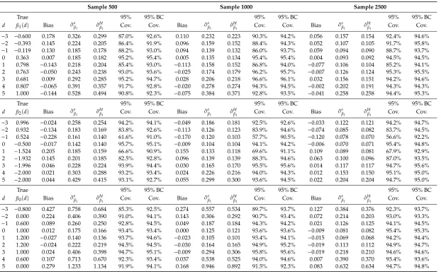
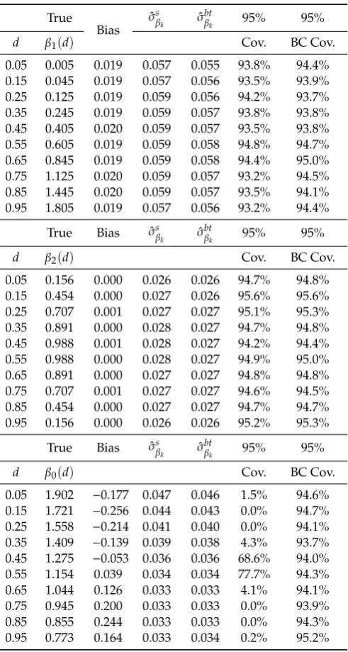
After each sample is simulated, the model is estimated with the procedure described in Section3, estimating the cross-validated bandwidths for each simulated sample, and estimating bootstrapped standard errors using 199 repetitions. Table1provides a summary of the results, showing the bias, standard errors from the simulations, average bootstrapped standard errors, and the 95% coverage and bias corrected coverage using normal based confidence intervals.
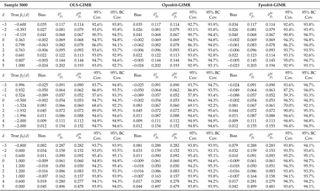
For the results in Table1, OLS-GIMR is used to correct for endogenous selection. Table2provides a similar exercise, using simulations with samples of size n=5000, but applying the GIMR from the ordered probit and fractional probit regression models. In all cases, Tables1and2reports the average estimates for the coefficients at selected points in the distribution ofd, with the top and bottom values (−3 and 5) representing the 2.5th and 97.5th percentiles of the distribution ofd.
The simulations suggest that the proposed estimator performs reasonably well in finite samples. Akin to other applications of semiparametric analysis, the estimator presents the largest bias at the boundaries of the distribution, but also around points where the second derivative of the coefficient with respect tod(∂2βk(d)/∂d2)is large. This bias disappears when larger samples and smaller bandwidths are used.
The bootstrap procedure used to correct the standard errors produces estimates that slightly understates the simulated standard errors. For the simulations with samples sizes n=500, the average bootstrapped standard errors understate the simulated standard errors by 5% in average. For the simulations with sample size of 5000, bootstrapped standard errors understate the simulated standard error in 2.5% in average. Looking at the raw coverage, except for areas with large bias, the estimator obtains coverages between 90% to 95%, even for the simulations with the smallest sample size.17 After correcting for the average bias, the coverage is above 94% for the majority of the cases. Finally, comparing the performance of the different estimators of the GIMR (Table2), all strategies perform similarly well, with only minor differences in coverage. Additional simulations presented in the appendix show that the choice of the GIMR estimations matters ifdhas a bounded distribution.18
17 Coverage estimates based on percentile confidence intervals show similar levels of coverage, and are not reported here. The simulation files are available upon request.
Table 1.Monte-Carlo Simulation summary. Based on OLS-Generalized Inverse Mills Ratios.
Sample 500 Sample 1000 Sample 2500
True 95% 95% BC 95% 95% BC 95% 95% BC
d β1(d) Bias σˆsβ1 σˆ bt
β1 Cov. Cov. Bias σˆ
s
β1 σˆ
bt
β1 Cov. Cov. Bias σˆ
s
β1 σˆ
bt
β1 Cov. Cov.
−3 −0.600 0.178 0.326 0.299 87.0% 92.6% 0.110 0.232 0.223 90.3% 94.2% 0.056 0.157 0.154 92.4% 94.6%
−2 −0.393 0.145 0.224 0.205 86.4% 91.9% 0.096 0.159 0.152 88.4% 94.3% 0.052 0.107 0.105 91.7% 95.8%
−1 −0.119 0.130 0.185 0.178 88.2% 93.0% 0.094 0.139 0.132 86.0% 93.7% 0.059 0.094 0.090 88.7% 93.7%
0 0.363 0.007 0.185 0.182 95.2% 95.4% 0.005 0.135 0.134 95.4% 95.4% 0.004 0.093 0.092 94.5% 94.5%
1 0.798 −0.143 0.218 0.204 85.4% 93.0% −0.113 0.158 0.152 86.8% 94.0% −0.077 0.106 0.104 85.2% 94.1%
2 0.763 −0.050 0.243 0.238 93.0% 93.6% −0.025 0.174 0.179 96.2% 95.7% −0.007 0.126 0.124 95.3% 95.5%
3 0.681 0.009 0.292 0.285 95.2% 94.7% 0.028 0.206 0.218 96.6% 96.1% 0.032 0.156 0.151 94.2% 94.6%
4 0.807 −0.065 0.391 0.357 91.7% 92.8% −0.020 0.278 0.274 94.3% 94.5% −0.002 0.202 0.191 94.3% 94.3%
5 1.000 −0.144 0.528 0.494 90.8% 92.3% −0.075 0.384 0.371 92.8% 93.5% −0.041 0.258 0.258 94.4% 95.3%
True 95% 95% BC 95% 95% BC 95% 95% BC
d β2(d) Bias σˆsβ1 σˆ bt
β1 Cov. Cov. Bias σˆ
s
β1 σˆ
bt
β1 Cov. Cov. Bias σˆ
s
β1 σˆ
bt
β1 Cov. Cov.
−3 0.996 −0.024 0.258 0.254 94.2% 94.1% −0.049 0.186 0.181 92.5% 92.6% −0.033 0.122 0.121 94.2% 94.7%
−2 0.932 −0.134 0.183 0.169 83.8% 92.6% −0.113 0.126 0.123 83.9% 94.6% −0.074 0.085 0.082 83.7% 94.5%
−1 0.524 −0.228 0.161 0.140 61.6% 91.0% −0.170 0.120 0.103 57.7% 90.5% −0.120 0.078 0.070 56.6% 92.2%
0 −0.500 −0.017 0.142 0.140 95.7% 95.1% −0.009 0.104 0.104 94.1% 94.2% −0.006 0.070 0.071 95.4% 94.8%
1 −1.524 0.205 0.185 0.159 66.6% 90.9% 0.155 0.133 0.118 69.6% 91.1% 0.109 0.089 0.081 67.9% 92.9%
2 −1.932 0.145 0.201 0.185 82.5% 92.8% 0.096 0.139 0.139 88.3% 94.6% 0.063 0.100 0.096 87.0% 93.5%
3 −1.996 0.046 0.228 0.224 93.9% 94.4% 0.030 0.165 0.170 95.5% 95.6% 0.014 0.117 0.117 94.7% 95.6%
4 −2.000 0.021 0.303 0.288 93.2% 93.4% 0.024 0.226 0.216 94.0% 94.3% 0.012 0.153 0.150 95.1% 95.0%
5 −2.000 0.044 0.429 0.415 93.1% 92.7% 0.055 0.299 0.300 93.6% 94.5% 0.022 0.204 0.204 94.7% 95.0%
True 95% 95% BC 95% 95% BC 95% 95% BC
d β0(d) Bias σˆsβ1 σˆ bt
β1 Cov. Cov. Bias σˆ
s
β1 σˆ
bt
β1 Cov. Cov. Bias σˆ
s
β1 σˆ
bt
β1 Cov. Cov.
−3 −0.800 0.427 0.758 0.684 85.3% 92.5% 0.274 0.557 0.534 89.7% 93.7% 0.127 0.384 0.376 92.3% 93.7%
−2 0.000 0.224 0.406 0.390 91.0% 94.1% 0.143 0.306 0.292 90.7% 93.4% 0.072 0.214 0.203 93.0% 93.3%
−1 0.600 0.089 0.260 0.250 92.8% 94.5% 0.049 0.187 0.184 94.3% 94.2% 0.021 0.126 0.125 94.1% 94.5%
0 1.000 0.012 0.175 0.166 93.4% 93.4% 0.000 0.125 0.121 93.6% 93.6% −0.009 0.081 0.082 95.4% 95.3%
1 1.200 −0.027 0.140 0.136 93.7% 94.6% −0.023 0.105 0.101 93.4% 94.1% −0.015 0.069 0.068 94.2% 94.4%
2 1.200 −0.024 0.222 0.219 94.5% 94.5% −0.030 0.164 0.165 94.9% 95.2% −0.019 0.113 0.112 94.9% 94.7%
3 1.000 0.024 0.406 0.398 94.7% 95.1% −0.009 0.294 0.306 95.8% 95.6% −0.019 0.218 0.210 94.6% 94.6%
4 0.600 0.107 0.713 0.670 92.3% 93.4% 0.037 0.538 0.525 94.0% 94.6% 0.007 0.390 0.370 93.4% 93.6%
5 0.000 0.279 1.233 1.134 91.9% 94.1% 0.168 0.946 0.892 91.5% 92.3% 0.083 0.632 0.634 94.7% 94.8%
Note: ˆσs
βkcorresponds to the simulated standard errors. ˆσ bt
βkcorresponds to the average bootstrapped standard errors. For each simulation, 199 repetitions are used to estimate bootstrapped
Table 2.Monte-Carlo Simulation summary: Alternative Generalized Inverse Mills Ratios estimates.
Sample 5000 OLS-GIMR Oprobit-GIMR Fprobit-GIMR
d Trueβ1(d) Bias σˆsβ1 σˆ bt
β1
95% Cov.
95% BC
Cov. Bias σˆ
s
β1 σˆ
bt
β1
95% Cov.
95% BC
Cov. Bias σˆ
s
β1 σˆ
bt β1 95% Cov. 95% BC Cov.
−3 −0.600 0.035 0.117 0.114 92.6% 93.8% 0.035 0.117 0.114 92.7% 93.9% 0.034 0.117 0.114 92.6% 93.8%
−2 −0.393 0.027 0.081 0.079 93.0% 93.8% 0.026 0.081 0.079 93.1% 93.8% 0.026 0.081 0.079 93.4% 93.9%
−1 −0.119 0.041 0.068 0.067 90.5% 94.5% 0.041 0.068 0.067 90.7% 94.4% 0.040 0.068 0.067 90.8% 94.5%
0 0.363 −0.002 0.069 0.068 94.5% 94.8% −0.002 0.069 0.069 94.5% 94.8% −0.002 0.069 0.069 94.3% 94.8%
1 0.798 −0.063 0.082 0.078 86.0% 94.1% −0.062 0.082 0.078 86.3% 94.0% −0.061 0.083 0.078 86.2% 94.0%
2 0.763 −0.006 0.095 0.092 93.6% 93.7% −0.006 0.096 0.093 93.6% 93.6% −0.006 0.096 0.093 93.7% 93.5%
3 0.681 0.022 0.122 0.113 93.0% 92.9% 0.022 0.122 0.113 93.0% 92.8% 0.022 0.123 0.114 93.1% 92.6%
4 0.807 −0.005 0.144 0.144 94.7% 94.6% −0.005 0.144 0.144 94.7% 94.7% −0.005 0.145 0.145 95.0% 94.7%
5 1.000 −0.024 0.202 0.193 93.0% 92.7% −0.024 0.202 0.193 92.9% 93.1% −0.023 0.203 0.194 92.9% 93.1%
d Trueβ2(d) Bias σˆsβ2 σˆ bt
β2
95% Cov.
95% BC
Cov. Bias σˆ
s
β2 σˆ
bt
β2
95% Cov.
95% BC
Cov. Bias σˆ
s
β2 σˆ
bt β2 95% Cov. 95% BC Cov.
−3 0.996 −0.025 0.091 0.090 93.7% 94.8% −0.025 0.091 0.090 93.7% 94.7% −0.024 0.091 0.090 93.6% 94.7%
−2 0.932 −0.050 0.064 0.062 86.8% 93.5% −0.050 0.064 0.062 86.8% 93.5% −0.049 0.064 0.063 87.2% 94.0%
−1 0.524 −0.089 0.057 0.052 57.6% 93.3% −0.089 0.057 0.052 57.8% 93.4% −0.088 0.057 0.052 59.3% 93.3%
0 −0.500 −0.002 0.054 0.053 94.7% 94.3% −0.002 0.054 0.053 94.6% 94.3% −0.002 0.054 0.053 94.5% 94.3%
1 −1.524 0.083 0.066 0.060 68.6% 92.2% 0.083 0.067 0.060 69.1% 92.2% 0.081 0.067 0.061 70.0% 92.1%
2 −1.932 0.045 0.072 0.072 89.0% 95.5% 0.045 0.072 0.072 89.2% 95.6% 0.044 0.072 0.072 90.0% 95.3%
3 −1.996 0.011 0.086 0.088 94.6% 94.6% 0.011 0.087 0.088 94.6% 94.6% 0.011 0.087 0.088 94.6% 94.8%
4 −2.000 0.009 0.111 0.112 94.9% 94.9% 0.009 0.111 0.112 94.9% 94.9% 0.009 0.111 0.113 94.8% 94.8%
5 −2.000 0.012 0.154 0.152 94.7% 94.6% 0.012 0.154 0.152 94.8% 94.6% 0.012 0.155 0.153 94.4% 94.5%
d Trueβ0(d) Bias σˆsβ0 σˆ bt
β0
95% Cov.
95% BC
Cov. Bias σˆ
s
β0 σˆ
bt
β0
95% Cov.
95% BC
Cov. Bias σˆ
s
β0 σˆ
bt β0 95% Cov. 95% BC Cov.
−3 −0.800 0.082 0.287 0.282 93.7% 93.9% 0.081 0.288 0.282 93.8% 93.9% 0.079 0.288 0.283 93.8% 94.1%
−2 0.000 0.034 0.158 0.152 93.0% 93.5% 0.033 0.159 0.152 93.1% 93.1% 0.032 0.159 0.153 93.5% 93.6%
−1 0.600 0.011 0.090 0.092 95.4% 95.1% 0.011 0.090 0.092 95.4% 95.1% 0.010 0.091 0.093 95.2% 95.1%
0 1.000 −0.009 0.061 0.060 94.8% 94.8% −0.009 0.061 0.060 94.9% 94.6% −0.009 0.061 0.061 94.8% 94.7%
1 1.200 −0.018 0.050 0.050 94.2% 95.4% −0.018 0.050 0.050 94.2% 95.3% −0.018 0.050 0.051 94.3% 95.5%
2 1.200 −0.016 0.086 0.083 93.3% 93.3% −0.016 0.086 0.083 93.3% 93.2% −0.016 0.086 0.083 93.4% 93.3%
3 1.000 −0.007 0.162 0.157 93.8% 93.9% −0.007 0.163 0.157 93.9% 93.8% −0.007 0.164 0.158 94.1% 93.7%
4 0.600 0.018 0.280 0.277 94.1% 94.3% 0.017 0.280 0.278 94.2% 94.2% 0.017 0.281 0.279 94.3% 94.2%
5 0.000 0.045 0.496 0.478 93.9% 94.0% 0.044 0.497 0.479 93.8% 93.9% 0.042 0.499 0.481 93.6% 94.1%
6. Application: Revising the Impact of Obesity on Wages
Several studies have found that that body weight is negatively correlated with wages, in particular for white women (Cawley 2004; Sabia and Rees 2012;Averett 2011;Fikkan and Rothblum 2012). The most common explanations for the negative correlation are: obesity lowers wages by reducing productivity and increasing discrimination; low wages may cause obesity due to unhealthy eating habits caused by lower income; or that unobserved factors simultaneously cause higher body weights and lower wages. On his review of the literature,Cawley(2004) criticizes the robustness of various strategies that have been followed in the literature to analyze the relationship between body weight and wages, and suggests the application of an instrumental variable approach to better capture the causal relationship between Body Mass Index (BMI) and wages.
Using data from the National Longitudinal Survey of the Youth (NLSY) for the years 1981 to 2000,Cawley(2004) provides estimations for the impact of BMI and weight on wages, using sibling’s BMI, sex and age as instruments for own BMI.19Correcting for reporting errors on weight and height, the evidence of his preferred model suggests that the negative effect of higher BMI on wages is only statistically significant for white women, with no statistically significant effect for other groups.
For the illustration of the proposed methodology, BMI will be considered the continuous group variable that is used to analyze the wage gaps in relation to body weight, using the same instrumental variables asCawley(2004). Due to the higher demands that the methodology imposes on the data, some changes on the data definitions and model specifications are introduced. These changes are described next.
6.1. Replication and Variable Definition Changes
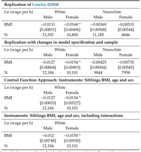
Cawley(2004) estimates instrumental variable models for six demographic groups based on gender and race, using measures for BMI that are corrected for self-reporting error20 as the main explanatory variable, and using siblings’ BMI, age and sex as instrumental variables. In his preferred model,Cawley(2004) reports that BMI has a negative impact on wages for all groups and races, but is only statistically significant for white woman. For this group, a one-point increase in BMI translates in 1.7% lower of wages.
Due to the higher demands that the semiparametric methodology imposes on the data, the original model specification required some adjustments.21 First, sampling weights are excluded from the analysis, so that clustered bootstrapped standard errors can be applied directly. Second, data with missing information in the general intelligence score, highest grade attained, job tenure and county employment rate are excluded from the sample. Father’s and mother’s highest degree of education are combined into a single variable (parent highest degree of education), and observations with missing data on both parents are also excluded from the sample. Finally, observations with a BMI below 14 and above 60 are also excluded from the sample. This reduces the total sample from 44,026 observations to 40,087 observations.
Re-estimating the results using the same specifications used inCawley(2004), incorporating the changes described above, show that the conclusions are robust to the model and sample specification changes, with small changes in the point estimates (see Table1). On the bottom two panels of Table3, the main model is re-estimated including the OLS-GIMR to account for endogeneity (Wooldridge 2015). OLS-GIMR is chosen because the full distribution of BMI is observed in the data. In addition to using the Siblings data as instruments, second order interactions are also included as instruments to account
19 The author implements a larger set of regression analysis using methodologies previously used in the literature. However, for the purpose of this paper, we will concentrate only on the instrumental variable approach. Further details on the data construction can be found inCawley(2004).
20 SeeCawley(2004, p. 454) for a complete description of the data and model specification.
for further nonlinear effects. The results using the OLS-GIMR are identical to the standard instrumental variable approach, showing only small changes when interactions are added as instruments. For the rest of the paper, linear and quadratic terms of the instrumental variables will be used to account for nonlinear effects for identification of the selection process.22
Table 3.Replication, Modified Specification, and Control Function estimations.
Replication ofCawley(2004)
Ln (wage per h) White Nonwhite
Male Female Male Female
BMI −0.0131 −0.0168 * −0.00369 −0.00515
[0.00831] [0.00496] [0.00508] [0.00544]
N 13,355 10,800 11,185 8686
Replication with changes in model specification and sample
Ln (wage per h) White Nonwhite
Male Female Male Female
BMI −0.0127 −0.0154 * −0.00425 −0.00735
[0.00804] [0.00493] [0.00504] [0.00545]
N 12,184 10,101 9844 7958
Control Function Approach: Instruments: Siblings BMI, age and sex
Ln (wage per h) White
Male Female
BMI −0.0127 −0.0154 *
[0.00833] [0.00527]
N 12,184 10,101
Instruments: Siblings BMI, age and sex, including interactions
Ln (wage per h) White
Male Female
BMI −0.012 −0.0150 *
[0.00748] [0.00530]
N 12,184 10,101
Note: Clustered standard errors at the individual level in parenthesis. Control function approach estimates use bootstrapped standard errors clustered at the individual level with 250 repetitions. *p<0.01.
6.2. Semiparametric Oaxaca Decomposition
6.2.1. Oaxaca Decomposition Approach and Implementation
To implement an OB decomposition in the present framework, it is necessary to define an appropriate reference group to analyze wage gaps across BMI, and the appropriate way to estimate the parameters for the reference group.23 For the analysis of BMI and wages, a common approach is to use individuals with a “healthy” BMI level as the baseline group, and compare the results against other groups (over and underweight). Following this premise, people with a BMI between 18.5 and 25 are used as the reference group, and the coefficients estimated with this sample will be considered as the average coefficients for people with healthy BMI. This group represents approximately 48% of
22 Control function approach using alternative measures for the GIMR were also estimated and are available upon request. While the results from the alternative specifications are similar to the ones presented here, they are somewhat larger and statistically significant for both white men and white women.
white men and 62% of white women. Using this reference group, the OB decomposition is obtained by estimating the following equations:
ln(wagei) =XiβH+δH∗λi+eii f BMIi ∈(18.5, 25) ln(wagei
BMIi =d) =Xiβ(d) +δ(d)∗λi+ei
(18)
The first equation is estimated using the sample of the reference group only (healthy BMI), whereas the second is estimated using kernel local linear regressions as described in Section4.1, over the whole distribution of BMI. Notice that both equations include the GIMR(λi)variable to adjust for sample selection, and that Equation (18) considers everyone, including those in the reference group.24
For the implementation of the OB decomposition, I use a threefold decomposition on the selectivity corrected wage gap, using the following formulas:
Composition effect : ∆X(d) =mˆx(d)−E(X
Healthy)βˆH
Wage Structure effect : ∆β =E(XHealthy)βˆ(d)−βˆH Interaction : ∆X(d)∆β= mˆx(d)−E(X
Healthy)βˆ(d)−βˆH
(19)
where ˆmx(d)is the local linear predicted mean ofXwith BMI atd, andE(X
Healthy)is the mean of X for people with healthy BMI, and ˆβHand ˆβ(d)are the estimated coefficients corresponding to the reference group and for people with BMI aroundd.
The bandwidth for the kernel regressions is selected separately for white men and white women using the cross-validation procedure described in Section4.2, using the OLS-GIMR as the selection correction term. To reduce impact of sparse areas in the distribution of BMI on the bandwidth selection, two approaches were taken. The first is to setω(Di) = 0 for observations at the top and bottom 1% of the distribution. The second is to use a strictly monotonic transformation of BMI, specifically the cumulative distribution G(BMI), as the grouping variable for the estimation of the local linear regressions.25 This transformation is similar to varying the bandwidth since more information will be used in areas that are more sparsely distributed than others, but it can also be compared to the use of k-nearest neighbors estimators. All models are estimated using Gaussian kernel functions. Table4provides the optimal bandwidths obtained from the cross-validation procedure for both men and women.26
Table 4.Cross-validated Optimal Bandwidths.
Variable of Reference Men CV Criterion Women CV Criterion
BMI 3.2900 −1.40814 4.8540 −1.56378
G(BMI) 0.1769 −1.40852 0.2241 −1.54543
Note: CV=Cross-validation Log of Mean Squared leave-one-out error.
6.2.2. Aggregate Decomposition Results
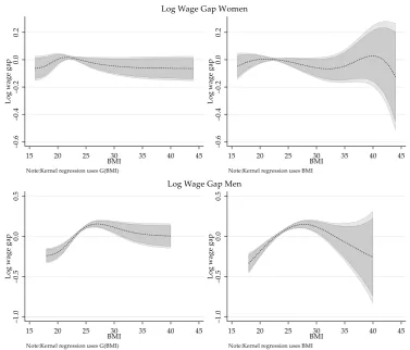
Figure1plots the selectivity corrected wage gap across the BMI for men and women, comparing people at all points of the BMI distribution with those in the reference group. The panels on the right provide the estimates that use the original BMI variable for the semiparametric regression, while the panels on the left show the estimates using the transformed variable G(BMI), but rescaled. The darker
24 This scenario assumes that BMI has no additional impact on wages within the health group. Alternatively, following the critique raised byCain(1986) in regards to using pooled data as the reference group, one could also include BMI as control in the pooled regression. For this illustration, such change has no substantial impact on the results.
25 In principle, this transformation should have no effect on the estimation of the semiparametric model. Ifz=g(x), andg()is a
strictly monotone transformation, thenE(y
X=x) =E(y
g(X) =g(x)) =E(y Z=z).
and lighter regions show the 90% and 95% confidence intervals constructed using a clustered paired bootstrap procedure with 399 repetitions. For men and women, the displayed gaps are provided for the relevant range of BMI which excludes the top and bottom 1% of the distribution.
According to the estimations, the selectivity corrected wage gap for men and women exhibit an inverse U shape with respect to their BMI. For women, I estimate a negative but non-statistically significant wage gap for all points of the BMI distribution. Based on the semiparametric estimation that relies on transformed BMI data, women at the top of the BMI distribution earn in average 6% less than the average women with healthy BMI, which is significant only at 10% level. The results based on kernel regressions with the original distribution of BMI provide qualitatively similar results but with lower precision at the extremes of the distribution.
In the case of men, the results suggest those with a BMI above 23 exhibit a positive and statistically significant wage gap compared to the reference group. The largest positive gap (16%) is observed for men with a BMI around 27, but this declines steadily for men with higher BMI, and turns statistically not significant for men with a BMI above 32. Men with a BMI below 22 show a negative wage gap, as large as 28% (based on the original variable distribution). Similar to the results for women, the estimates for men at the top of the BMI distribution are less precise when using the original BMI for the semiparametric regression. Because the results using the transformed variable are more precise than the alternative, the rest of the analysis will center on these estimations alone.27
Econometrics 2019, 7, x FOR PEER REVIEW 15 of 28
and lighter regions show the 90% and 95% confidence intervals constructed using a clustered paired bootstrap procedure with 399 repetitions. For men and women, the displayed gaps are provided for the relevant range of BMI which excludes the top and bottom 1% of the distribution.
According to the estimations, the selectivity corrected wage gap for men and women exhibit an inverse U shape with respect to their BMI. For women, I estimate a negative but non-statistically significant wage gap for all points of the BMI distribution. Based on the semiparametric estimation that relies on transformed BMI data, women at the top of the BMI distribution earn in average 6% less than the average women with healthy BMI, which is significant only at 10% level. The results based on kernel regressions with the original distribution of BMI provide qualitatively similar results but with lower precision at the extremes of the distribution.
In the case of men, the results suggest those with a BMI above 23 exhibit a positive and statistically significant wage gap compared to the reference group. The largest positive gap (16%) is observed for men with a BMI around 27, but this declines steadily for men with higher BMI, and turns statistically not significant for men with a BMI above 32. Men with a BMI below 22 show a negative wage gap, as large as 28% (based on the original variable distribution). Similar to the results for women, the estimates for men at the top of the BMI distribution are less precise when using the original BMI for the semiparametric regression. Because the results using the transformed variable are more precise than the alternative, the rest of the analysis will center on these estimations alone.27
27 Figures in Appendix B provide various robustness checks including: Sensitivity to alternative GIMRs,
results based on kernel regressions with original BMI distribution, and differences in the bandwidth estimation.
Figure 1.Selectivity corrected Wage gap over BMI by gender. Note: Darker and lighter areas correspond to the 90% and 95% confidence intervals. Confidence intervals constructed based on bootstrapped standard errors with 399 repetitions clustered at the individual level.
Econometrics2019,7, 28 16 of 29
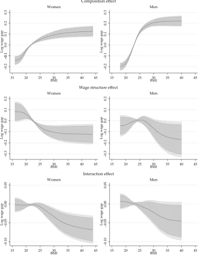
Similar to the standard OB analysis, the total wage gap reported in Figure1is not an adequate measure of the wage gap driven by differences in BMI because it is are driven by differences in characteristics (composition effect), coefficients (wage structure effect) or a combination of both. On Figure2, I provide the semiparametric estimations for these three components for men and women.
Figure 1. Selectivity corrected Wage gap over BMI by gender. Note: Darker and lighter areas correspond to the 90% and 95% confidence intervals. Confidence intervals constructed based on bootstrapped standard errors with 399 repetitions clustered at the individual level.
Similar to the standard OB analysis, the total wage gap reported in Figure 1 is not an adequate measure of the wage gap driven by differences in BMI because it is are driven by differences in characteristics (composition effect), coefficients (wage structure effect) or a combination of both. On Figure 2, I provide the semiparametric estimations for these three components for men and women.
Figure 2. Aggregated Semiparametric decomposition components. Note: Darker and lighter areas correspond to the 90% and 95% confidence intervals. Confidence intervals constructed based on bootstrapped standard errors with 399 repetitions clustered at the individual level.
distribution of BMI, differences in characteristics explain a wage gap that ranges between−20% to 21% for men, and−14% to 12% for women, when looking at people with BMI of 18 and 40, and compared to people with healthy BMI. This implies that white men and women with higher BMI have on average better endowments, which translates into higher wages.
Consistent with Cawley (2004) estimates, the wage structure effect for women shows a monotonically decreasing trend respect to BMI across the whole distribution, suggesting that BMI has a negative but non-linear impact on wages. The estimations show that there is a steady decline in the wage structure component among women, with a wage gap that goes from+8% for women with BMI of 18, to a wage gap of−11% for women with a BMI of 30.
For men, the effect of BMI on wages shows a different pattern. On the one hand, the results are less precise and the wage structure effect is not statistically significant across BMI. Setting aside the low precisions of the estimates, the wage structure effect for men shows an inverse u shape with respect to BMI. Compared to men with a BMI of 25, for whom a point estimate of+0.7% wage structure gap is estimated, the wage premium declines at lower and higher ends of BMI distribution. This may explain why the instrumental variable estimates for men’s (see Table3) is negative but not statistically significant.
The last component of the decomposition is the interaction effect, which accounts for the fact that average wages are different because both coefficients and characteristics differ across groups. For men and women, the interaction effect grows negative with higher BMI, but it is only statistically significant for women.
6.2.3. Revisiting the Impact of Obesity on Wages: Partial Effect of BMI
One of the conclusions inCawley(2004) is that a one standard deviation increase in body weight (roughly 32lbs), or equivalently a 5.5 BMI points increase, is associated with a drop in wages of 9%.28 This is a linear extrapolation of the estimates of their preferred model which suggest that a one-point increase in BMI is associated with a wage reduction of 1.7%.
While the results provided on Figure2cannot be directly compared to these findings, a modification of the wage structure effect in Equation (19) can be used to obtain partial effects that can be directly compared to Cawley’s results. Specifically, using characteristics fixed to the reference group, the marginal effect of BMI on the wage structure effect can be calculated as follows:
∂Wage Gap(∆β) ∂BMI
BMI=d
=E(XHealthy) ˆ
β(d+ε)−βˆ(d−ε)
ε
!
(20)
Figure3provides the estimations of the change of the wage structure effect as a function of BMI, and compares them to the marginal effect based on the replication of the IV linear estimates presented in Table3.29
28 Cawley(2004, p. 465) stated that a two standard-deviation change in weight is associated with a 9 percent change in wages, when in fact this estimate reflects the impact of a one standard-deviation change in weight.
Econometrics 2019, 7, x FOR PEER REVIEW 18 of 28
Figure 3. Partial effect of BMI on the Wage Structure effect. Note: Darker and lighter areas correspond to the 90% and 95% confidence intervals for the linear IV estimate and the semiparametric estimate. Confidence intervals are constructed using the delta method and are based on Bootstrapped standard errors with 399 repetitions clustered at the individual level. The vertical axis measures the marginal effect of BMI on the wage structure component of the wage gap.
The marginal effect of BMI on the wage structure for women with a BMI between 20 and 25 is larger than that based on the linear IV estimate. The largest estimated marginal effect indicates that one-point increase in BMI for a woman with a BMI score of 22.5 relates to a wage decline of 2.5%, an almost 65 percent greater effect than linear IV estimate (1.5%). The negative impact of increasing BMI is not statistically significant for women with BMI below 20 or above 29, and the impact is below 0.5% for women with a BMI below 18 or above 30. Men with a BMI below 25 seem to experience a small positive wage gain associated with increasing BMI, although it is not statistically significant. The wage penalty due to a higher BMI is statistically significant above 27, with the largest wage decline is measured at 2.3% (at a BMI of 29.5), almost twice as large as the linear IV estimates of 1.2%. While the partial effect on wages decrease as BMI increases, it remains statistically significant through the rest of the BMI distribution.
7. Conclusions
In this paper, I have presented a methodology for the implementation of Oaxaca–Blinder decomposition when the grouping variable is continuous, and there is presence of endogenous selection into groups. This methodology uses a semiparametric approach known as varying coefficient models (Hastie and Tibshirani 1993), which has the advantage to provide a more flexible specification on the parameterization of the coefficients, compare to the models proposed by Ñ opo (2008) and Ulrick (2012). Specifically, this paper describes the use of kernel local linear regressions for the estimation of such models.
The use of the generalized inverse mills ratios, also known as generalized residuals, allow for a feasible strategy to control for the endogenous selection based on the continuous grouping variable. This methodology is similar to the one proposed in Delgado et al. (2019), suggesting a similar control function approach to address endogeneity from the semiparametric component of the regression. While I do not discuss the theoretical properties of the estimator, the Monte-Carlo Simulation exercises suggests that the proposed strategy provides a simple but powerful approach to obtain consistent estimators of the outcome model parameters. This suggests that the proposed estimator can be used alongside to the methodologies proposed by Centorrino and Racine (2017) and Delgado et al. (2019). A more formal analysis of theoretical properties of the proposed estimator is left for future research.
This methodology may prove useful for the analysis of endogenous treatment effects with varying treatment intensity, when heterogeneous effects are present. In addition, it can also be used Figure 3.Partial effect of BMI on the Wage Structure effect. Note: Darker and lighter areas correspond to the 90% and 95% confidence intervals for the linear IV estimate and the semiparametric estimate. Confidence intervals are constructed using the delta method and are based on Bootstrapped standard errors with 399 repetitions clustered at the individual level. The vertical axis measures the marginal effect of BMI on the wage structure component of the wage gap.
The marginal effect of BMI on the wage structure for women with a BMI between 20 and 25 is larger than that based on the linear IV estimate. The largest estimated marginal effect indicates that one-point increase in BMI for a woman with a BMI score of 22.5 relates to a wage decline of 2.5%, an almost 65 percent greater effect than linear IV estimate (1.5%). The negative impact of increasing BMI is not statistically significant for women with BMI below 20 or above 29, and the impact is below 0.5% for women with a BMI below 18 or above 30. Men with a BMI below 25 seem to experience a small positive wage gain associated with increasing BMI, although it is not statistically significant. The wage penalty due to a higher BMI is statistically significant above 27, with the largest wage decline is measured at 2.3% (at a BMI of 29.5), almost twice as large as the linear IV estimates of 1.2%. While the partial effect on wages decrease as BMI increases, it remains statistically significant through the rest of the BMI distribution.
7. Conclusions
In this paper, I have presented a methodology for the implementation of Oaxaca–Blinder decomposition when the grouping variable is continuous, and there is presence of endogenous selection into groups. This methodology uses a semiparametric approach known as varying coefficient models (Hastie and Tibshirani 1993), which has the advantage to provide a more flexible specification on the parameterization of the coefficients, compare to the models proposed byÑopo(2008) and Ulrick(2012). Specifically, this paper describes the use of kernel local linear regressions for the estimation of such models.
The use of the generalized inverse mills ratios, also known as generalized residuals, allow for a feasible strategy to control for the endogenous selection based on the continuous grouping variable. This methodology is similar to the one proposed inDelgado et al.(2019), suggesting a similar control function approach to address endogeneity from the semiparametric component of the regression. While I do not discuss the theoretical properties of the estimator, the Monte-Carlo Simulation exercises suggests that the proposed strategy provides a simple but powerful approach to obtain consistent estimators of the outcome model parameters. This suggests that the proposed estimator can be used alongside to the methodologies proposed byCentorrino and Racine(2017) andDelgado et al.(2019). A more formal analysis of theoretical properties of the proposed estimator is left for future research.