www.ocean-sci.net/9/931/2013/ doi:10.5194/os-9-931-2013
© Author(s) 2013. CC Attribution 3.0 License.
Ocean Science
The circulation of Icelandic waters – a modelling study
K. Logemann1, J. Ólafsson1,2, Á. Snorrason3, H. Valdimarsson2, and G. Marteinsdóttir1
1School of Engineering and Natural Sciences – University of Iceland, Reykjavik, Iceland 2Marine Research Institute Iceland, Reykjavik, Iceland
3Icelandic Meteorological Office, Reykjavik, Iceland Correspondence to: K. Logemann ([email protected])
Received: 20 March 2013 – Published in Ocean Sci. Discuss.: 19 April 2013
Revised: 10 September 2013 – Accepted: 3 October 2013 – Published: 30 October 2013
Abstract. The three-dimensional flow, temperature and salinity fields of the North Atlantic, including the Arctic Ocean, covering the time period 1992 to 2006 are simu-lated with the numerical ocean model CODE. The simula-tion reveals several new insights and previously unknown structures which help us to clarify open questions on the re-gional oceanography of Icelandic waters. These relate to the structure and geographical distribution of the coastal current, the primary forcing of the North Icelandic Irminger Current (NIIC) and the path of the Atlantic Water south-east of Ice-land. The model’s adaptively refined computational mesh has a maximum resolution of 1 km horizontal and 2.5 m vertical in Icelandic waters. CTD profiles from this region and the river discharge of 46 Icelandic watersheds, computed by the hydrological model WaSiM, are assimilated into the simula-tion. The model realistically reproduces the established ele-ments of the circulation around Iceland. However, analysis of the simulated mean flow field also provides further insights. It suggests a distinct freshwater-induced coastal current that only exists along the south-west and west coasts, which is accompanied by a counter-directed undercurrent. The sim-ulated transport of Atlantic Water over the Icelandic shelf takes place in a symmetrical system of two currents, with the established NIIC over the north-western and northern shelf, and a hitherto unnamed current over the southern and south-eastern shelf, which is simulated to be an upstream precur-sor of the Faroe Current (FC). Both currents are driven by barotropic pressure gradients induced by a sea level slope across the Greenland–Scotland Ridge. The recently discov-ered North Icelandic Jet (NIJ) also features in the model pre-dictions and is found to be forced by the baroclinic pressure field of the Arctic Front, to originate east of the Kolbeinsey Ridge and to have a volume transport of around 1.5 Sv within
northern Denmark Strait. The simulated multi-annual mean Atlantic Water transport of the NIIC increased by 85 % dur-ing 1992 to 2006, whereas the corresponddur-ing NIJ transport decreased by 27 %. Based on our model results we propose a new and further differentiated circulation scheme of Ice-landic waters whose details may inspire future observational oceanography studies.
1 Introduction
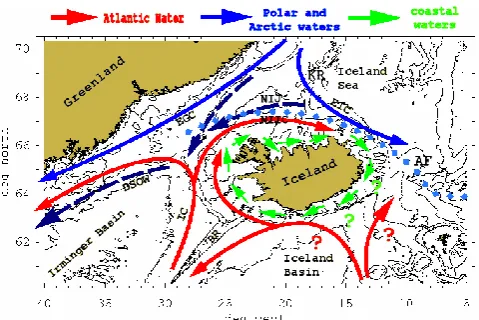
The waters surrounding Iceland, flowing over the shelf and along the adjacent continental slope, form one of the hydro-graphically most complicated regions of the North Atlantic. The primary drivers of this complexity are topography and the interaction of four water masses. Iceland is located at the junction of the Mid-Atlantic Ridge and the Greenland– Scotland Ridge, which segments the adjacent Atlantic into four basins bounded by the Reykjanes Ridge to the south, the Kolbeinsey Ridge to the north, the Greenland–Iceland Sill (Denmark Strait) to the west and the Iceland–Faroe Ridge to the east (Fig. 1).
932 K. Logemann et al.: The circulation of Icelandic waters
Fig. 1. Bathymetry around Iceland and the classical view of the ocean circulation. The isobaths are: 200, 500, 1000, 2000 and 3000 meters. The abbreviations are: AF – Arctic Front, DSOW – Den-mark Strait Overflow Water, EGC – East Greenland Current, EIC – East Icelandic Current, IC – Irminger Current, KR – Kolbein-sey Ridge, NIIC – North Icelandic Irminger Current, NIJ – North Icelandic Jet, RR – Reykjanes Ridge. The question marks indicate questionable structures like the coastal current. Modified after Lo-gemann and Harms (2006).
Subpolar Mode Water northwards. The IC volume flux was estimated at 19±3 Sv by Våge et al. (2011a). The associated northward heat flux plays a crucial role for the marine and terrestrial climate of Iceland. South of Denmark Strait, the IC mostly recirculates towards the west and further south-wards along the East Greenland continental slope. However, a small fraction (5–10 %) of the current branches off north-wards through Denmark Strait and further eastnorth-wards over the North Icelandic shelf (Kristmannsson, 1998). This branch, called the North Icelandic Irminger Current (NIIC), is re-sponsible for the mild climate north of Iceland and forms, to a certain extent, the lifeline of the local marine ecosystem (Vilhjálmsson, 1997).
In normal years, the Atlantic Water of the NIIC, with some admixture of Polar Water entrained in Denmark Strait, dom-inates most of the North Icelandic shelf area. However, on its eastward journey over the northern shelf the admixture of the second water mass, the Arctic Intermediate Water, becomes more and more important. This water mass, often also termed Arctic waters, is formed of Atlantic Water which moved into the Nordic seas, mainly over the Faroe–Iceland Ridge and through the Faroe–Shetland Channel (Orvik et al., 2001), several years prior and has been exposed to atmo-spheric cooling and freshwater addition in the interior Green-land and IceGreen-land seas since that time. It is therefore colder (T:
−1 to 4◦C) and slightly fresher (S34.6 to 34.9) than the At-lantic Water (Swift, 1986). The East Icelandic Current (EIC) carries Arctic Intermediate Water, with an admixture of Po-lar Water, from the central Iceland Sea southwards along the eastern flank of the Kolbeinsey Ridge onto the north-eastern
Icelandic shelf, causing the water here to be characteristi-cally more Arctic than Atlantic. Thereafter, the EIC, whose volume flux was measured to be 2.5 Sv between June 1997 and June 1998 (Jónsson, 2007), continues towards the north-ern flank of the Iceland–Faroe Ridge.
East of Iceland the Arctic waters of the EIC border on the Atlantic Water of the Faroe Current (FC) which flows east-wards along the northern flank of the Iceland–Faroe Ridge. The front between the cold Arctic waters to the north and the warm Atlantic Water of the NIIC and FC to the south is called Arctic Front and is characterised by sharp temper-ature gradients (Hansen and Meincke, 1979; Orvik et al., 2001). The resulting density gradient leads to differences in sea level height, with higher values to the warmer and less dense southern side of the front. The Arctic Front contin-ues south-eastwards along the Iceland–Faroe Ridge, to the region north of the Faroe Islands. Westwards it extends north of Iceland up to Denmark Strait where it opens out into the Polar Front (Fig. 1). Below the NIIC there exists a deep un-dercurrent which carries Arctic waters westwards along the north Icelandic continental slope from east of the Kolbeinsey Ridge up to Denmark Strait. This current, discovered only in 2004 (Jónsson and Valdimarsson, 2004), is called the North Icelandic Jet (NIJ) and seems to make a crucial contribution to the Denmark Strait Overflow, a key element of the Atlantic meridional overturning circulation (Våge et al., 2011b).
The third water mass is Polar Water that originates in the surface layer of the Arctic Ocean. Here, the freshwater dis-charge of the great Siberian and Canadian rivers forms very fresh (S <34.4) and, due to atmospheric cooling, very cold (T <0◦C) surface water. A part of this water mass leaves the Arctic Ocean with the East Greenland Current (EGC) which flows southwards over the East Greenland shelf, thereby forming the Polar Front at the interface to the adjacent Arc-tic and AtlanArc-tic water masses (Swift, 1986). Hence, the bulk of the Polar Water, which is mostly ice covered, passes Ice-land along the western side of the Denmark Strait whereas smaller parts mix into the NIIC to the east (Logemann and Harms, 2006; Jónsson and Valdimarsson, 2012). This seems to happen mainly in the form of cold and fresh eddies sepa-rating from the Polar Front (Våge et al., 2013). Furthermore, the variable wind field north of Denmark Strait may cause events of eastward drift of Polar Water onto the North Ice-landic shelf. The Polar Water was in fact observed to dom-inate the North Icelandic shelf during the period between 1965 and 1971 (Malmberg and Kristmannsson, 1992).
has prevailed since 1996, with a trend of increasing stability (Jónsson and Valdimarsson, 2012).
The fourth and final water mass is coastal water. The freshwater discharge along the Icelandic coast produces low-salinity near-shore water which is enriched by the river-borne silicate (Ólafsson et al., 2008). The classical view of the circulation pattern is that the coastal water flows clock-wise around the island (Fig. 1). A discrete coastal current, driven by the barotopic pressure field related to a freshwa-ter induced coastal density front, has been observed sev-eral times (Ólafsson, 1985; Ólafsson et al., 2008) and nu-merous satellite images (e.g., at the NASA MODIS project gallery, http://modis.gsfc.nasa.gov/) show the appearance of a distinct coastal water mass, visible through a combination of algal bloom and riverine suspended matter. However, the temporal variability and geographical distribution of this wa-ter mass and its accompanying ocean current, the Icelandic Coastal Current (ICC), is still unclear. Further, even the cept of the continuous circular clockwise flow seems to con-tradict drift observations at the south-east coast of Iceland (Valdimarsson and Malmberg, 1999).
The importance of the coastal water and its flow for the marine ecosystem is beyond dispute. The nutrients it con-tains, along with the stratifying effect of the freshwater on the water column, are thought to be important elements of the spring algal bloom in Icelandic waters (Þórðardóttir, 1986). Furthermore, the flow acts as a dispersal vector for fish eggs and larvae transported away from spawning grounds to their nursery areas, and hence plays a crucial role in the recruit-ment process of several fish species in Icelandic waters (Ólaf-sson, 1985; Marteinsdóttir and Astþór(Ólaf-sson, 2005).
The uncertainty over the structure of the ICC is a key mo-tivation for the present study. We also explore the general forcing of the NIIC, a current flowing northwards against the prevailing wind direction (Fig. 14) and a subject of intensive research for more than 50 yr due to its exceptional hydro-graphical and ecological importance for North Icelandic wa-ters (e.g., Stefánsson, 1962; Kristmannsson, 1998; Ólafsson 1999, Jónsson and Valdimarsson 2005, 2012, Halldórsdóttir, 2006; Logemann and Harms 2006). Furthermore, we exam-ine the structure of the relatively unexplored NIJ and the path of the Atlantic Water flow towards the south and south-east coast of Iceland, a controversial component of the regional hydrography (e.g., Valdimarsson and Malmberg, 1999; Orvik and Niiler, 2002; Hansen et al., 2003).
To address these objectives we need to explore and un-derstand the three-dimensional flow, temperature and salinity fields of the waters surrounding Iceland and beyond. We use the tool of numerical ocean modelling, which offers the pos-sibility to obtain the requested fields with high temporal and spatial resolution covering large areas and long time periods. The most established numerical model of Icelandic waters is a two-dimensional application of the POM ocean model (Blumberg and Mellor, 1978). It was set up for Icelandic wa-ters by Tómasson and Eliasson (1995) and further improved
by Tómasson and Káradóttir (2005). The model is run on an operational basis at the Icelandic Maritime Administration to predict tidal and atmospherically forced sea level elevations and currents.
The first three-dimensional model study on Icelandic wa-ters was performed by Mortensen (2004). By using an appli-cation of the MIKE3 (Rasmussen, 1991) ocean model with a resolution of 20 km horizontal and 50 m vertical his study mainly dealt with the circulation in Denmark Strait, with vol-ume, heat and salt fluxes of the EGC and the Denmark Strait Overflow.
In 2006 three further modelling studies on Icelandic wa-ters were published. Ólason (2006) set up the MOM4 ocean model (Griffies et al., 2004) for the region with a resolution of around 15 km horizontal and 10 m vertical near the sea surface. Driven by climatological wind fields the model suc-cessfully reproduced the basic elements of the circulation. Sensitivity experiments regarding the role of the local wind stress in forcing the near surface circulation were carried out. Halldórsdóttir (2006) applied the same model whereas her numerical experiments examined the dynamic impact of the coastal freshwater and the sensitivity of the NIIC to wind stress variations. Eventually, Logemann and Harms (2006) published their work on the high-resolution (1 km horizon-tal, 10 m vertical) simulation of the NIIC with the ocean model CODE. Time and space variability of the NIIC vol-ume and heat fluxes for the years 1997–2003 were analysed and the origin and composition of NIIC water masses were estimated.
For the following years the development work on the CODE model with focus on Icelandic waters was carried on (Logemann et al., 2010, 2012) which finally led to the ver-sion whose output is presented here. This resolves the entire coastal area with a grid spacing of 1 km horizontal and 2.5 m vertical. It uses coastal freshwater discharge values computed by a newly developed high-resolution application of the hy-drological model WaSiM (Schulla and Jasper, 2007; Einars-son and JónsEinars-son, 2010) and it assimilates hydrographic mea-surements like CTD (conductivity, temperature, depth) pro-files into the simulation.
Therefore, we propose that these model results could throw new light on the above-mentioned questions and even enable us to propose previously unobserved structures of the regional hydrography of Icelandic waters.
2 Model description
934 K. Logemann et al.: The circulation of Icelandic waters
The basis of the model is formed by the primitive equa-tions (Bjerknes, 1921), i.e. non-linear, incompressible, for-mulations of the Navier–Stokes equations, which are used to approximate the oceanic flow in Cartesian coordinates (x, y, z) in a hydrostatic pressure field. In order to simu-late tides the tidal potential, given by a first order approach (Apel, 1987), was added. Here, we set the solar and lunar co-declinations to time invariant constants which reduces the tidal spectrum mainly to the M2and S2constituents
(Loge-mann et al., 2012). The density of seawater as a function of salinityS, temperatureT and hydrostatic pressure is com-puted with the EOS-80 equations by Millero et al. (1980).
Temperature and salinity changes are computed with (e.g., Pedlosky, 1987)
∂T ∂t = −u
∂T ∂x −v
∂T ∂y −w
∂T ∂z +0
+ ∂
∂x KH, T ∂T ∂x + ∂ ∂y
KH, T ∂T∂y
+ ∂
∂z
KV, T (∂T∂z +0)
+QT,
(1)
∂S ∂t = −u
∂S ∂x−v
∂S ∂y −w
∂S ∂z +
∂ ∂x KH,S
∂S ∂x + ∂ ∂y KH,S ∂S∂y
+ ∂
∂z
KV,S ∂S∂z
+QS,
(2)
in which (u, v, w) is the three-dimensional flow vector and 0=0(T , S, p) is the adiabatic lapse rate, computed with the equation of Fofonoff and Millard (1983), whereas QT and
QS denote the sum of surface heat and freshwater fluxes,
re-spectively. These fluxes are derived by the atmospheric forc-ing (wind, air temperature, humidity, cloudiness) usforc-ing the bulk formulas after Gill (1982). The coefficients of horizon-tal turbulent exchange, KH, T and KH,S, are estimated
us-ing the approach of Smagorinsky (1963), the coefficients of vertical turbulent exchange,KV, T andKV, S, are computed
after Pohlmann (1996) based on the approach of Kocher-gin (1987).
The current CODE version uses a dynamic thermody-namic sea ice model based on the work of Hibler (1979). Whereas the thermodynamic part (ice growth and melting) is coupled to the oceanic surface heat flux QT in Eq. (1)
the dynamic part contains a viscous-plastic rheology in or-der to compute the ice drift and rafting forced by the wind, the ocean currents and the sea surface elevation gradient (Logemann et al., 2010).
2.1 Numerics
The model equations are numerically solved with the tech-nique of finite differences in Cartesian coordinates. A three-dimensional staggered Arakawa-C-grid (Mesinger and Arakawa, 1976) with a spatially variable resolution is con-structed. The equations’ numerical equivalents are formu-lated centred in space and mostly implicit in time. In order to avoid numerical diffusion of the advection terms a flux limiter function (van Leer, 1979) is used, which ensures the abidance of the total variation diminishing (TVD) condition.
2.1.1 Adaptive mesh refinement and model domain
CODE uses a technique of adaptive mesh refinement which is oriented at the “tree-algorithm” of Khokhlov (1998). This algorithm starts with a model domain being divided by a reg-ular three-dimensional computational mesh of basic cells. If there is an area which demands a higher resolution, each ba-sic cell of this area is split into eight “children” with halved side lengths. Some of these children may be split further, each of them into eight “grandchildren”, those perhaps into “great-grandchildren” and so on, until the area of interest is resolved with the desired resolution. The model equations are only solved for “childless” cells, but the “parent” cells are not removed from the computer memory. At each time step, they obtain the average properties of their children instead. These values may be used for numerical operations at coarser parts of the mesh.
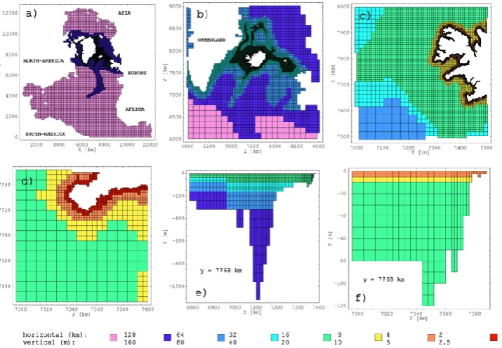
The actual form of adaptive mesh refinement is static, i.e., it does not vary in time, and just follows geographi-cal criteria. By using five different stereographic projections, with their projection points along the 40◦W meridian and weighted by a latitude dependent function, a Cartesian co-ordinates model domain containing the entire North Atlantic including the Arctic Ocean was constructed (Fig. 2). This do-main is resolved by a basic mesh with a spacing of 128 km horizontal and 160 m vertical. First the cell thickness is re-fined up to 2.5 m close to the sea surface then the horizon-tal and deeper vertical mesh structure is further refined in selected regions. The refinement begins in the Nordic Seas, the Irminger and Iceland Basin, the Canadian Archipelago and along the northern Mid-Atlantic Ridge, continues with further refinement along the Greenland–Iceland–Scotland Ridge and finally leads to a mesh with 1 km horizontal and 2.5 to 10 m vertical resolution along the Icelandic coast (Fig. 2).
2.1.2 Data assimilation
The simulated temperatures and salinities at a certain dis-tance from Iceland, i.e. the area south of 60◦N, north of 70◦N, west of 30◦W and east of 5◦W, are restored to the climatologic fields of the PHC 3.0 (Polar Science Center Hydrographic Climatology) data set (Steele et al., 2001). This data set, compiled in 2005, combines the “Word Ocean Atlas” (1998 edition), the “Arctic Ocean Atlas” and se-lected Canadian data provided form the Bedford Institute of Oceanography and therefore forms an appropriate resource for the simulation of the North Atlantic/Arctic Ocean (Li et al., 2011). The restoring consists of a 365-day Newtonian scheme towards the 12 monthly fields of the PHC.
Fig. 2. The computational mesh in Cartesian coordinates. Different colours are used to identify the different resolutions. (a) The entire model domain. (b–d) The horizontal refinement. (e–f) The vertical refinement along a section west of Iceland.
data set (ICES, 2000)) and extracted 16,802 CTD (conduc-tivity, temperature, depth) profiles from the period 1992 to 2006 recorded between 60◦N and 70◦N and between 30◦W and 5◦W. This meant that 93 profiles per simulated month were available on average with May and June being the best-surveyed months with on average 206 and 143 profiles, re-spectively whereas December and January show the lowest numbers, 30 and 23, respectively. With the help ofT /S and latitude/longitude diagrams the quality of the input data and its processing into the model was checked. No spikes or other great errors were detected which is not surprising consider-ing the fact that, before delivery to the data base, a standard high level quality control was performed by each data con-tributor and an additional data cleaning has been applied to the data sets afterwards (ICES, 2000; Nilsen et al., 2006).
In order to adjust the model towards these observa-tions we used the data assimilation technique of IAU (incremental analysis updating) processes (Bloom et al., 1996). Though more sophisticated methods like the “Prac-tical Global State Estimation” (Wunsch and Heimbach, 2007) may have led to better results we decided to start the related model development with the implementation of a rather simple, straightforward and computationally less intensive algorithm. The model performing a “free forecast” simulation was stopped when having reached the 15th of a month. The CTD data of this month, i.e. from the 1 to the 30, was bundled and compared with the simulated fields. Based on the assumption that the differences between the simulation and the calibrated high
quality CTD profiles are close to the true model error, the profiles of temperature and salinity difference were horizontally interpolated, in order to create estimates of the three-dimensional temperature and salinity error fields. The model was jumped one month back in time and the simulation re-started, but now with the correction terms 1u, 1v, 1w, 1 KH, T, 1 KH,S, 1 KV, T, 1 KV, S, 1QT, 1QS
determined for every grid cell at every time step in order to correct the flow field, mixing rates or surface fluxes. These terms essentially are functions of the horizontally interpolated error field and the simulated difference from the free forecast. A detailed description of their computation is given in Logemann et al. (2012).
This way, Eq. (1) becomes ∂T
∂t = −(u+1u) ∂T
∂x −(v+1v) ∂T
∂y −(w+1w)
∂T
∂z+0
+∂ ∂x
KH, T+1KH, T
∂T
∂x
+ ∂ ∂y
KH, T+1 KH, T
∂T
∂y
+∂ ∂z
(KV, T+1 KV, T)( ∂T
∂z+0)
+QT+1QT+1QNUMT ,
(3)
936 K. Logemann et al.: The circulation of Icelandic waters
Fig. 3. Winter (left panel) and summer (right panel) mean discharge of 46 Icelandic watersheds for the time period 1992 to 2006 simulated with WaSiM. Below the simulated mean seasonal signal of the island’s overall discharge for the same time period is shown.
and CTD data is reduced from initial−0.989 K (0.176) to
−0.233 K (0.038) after the third iteration. The correction term1QNUMdenotes additional corrections of the simulated temperature or salinity, being activated during the last two it-erations, having the function of “un-physically” correct nu-merical errors like nunu-merical diffusion or erroneous initial or boundary conditions.
3 Simulation of the period 1992–2006
3.1 Setup
The two oceanic boundaries of the model domain – slightly south of the equator between South America and West Africa and across Bering Strait in the Arctic – are treated as closed boundaries. Because of the far field restoring towards cli-matological values, the hydrodynamic implications of these boundary conditions are assumed to be negligible for Ice-landic waters. Initial model data, describing the summer 1991, were taken from a model run performed by a previous model version (Logemann et al., 2010).
The atmospheric forcing of the model consists of the 6-hourly NCEP/NCAR re-analysis fields (Kalnay et al., 1996). This state-of-the-art data set (Hodges at al., 2011; Mooney et al., 2011; Tilinia et al., 2013) was chosen because it stretches back to the year 1948 and therefore allows a greater flexi-bility in the setup of future hindcast simulations. The model reads in the following seven parameters: precipitation rate, specific humidity (2 m), sea level pressure, air temperature
(2 m), total cloud cover, zonal and meridional wind speed (10 m).
During the simulation, three-hourly means of the physical ocean state, including sea ice properties, were stored. The averaging period of three hours was chosen to resolve tidal dynamics.
Icelandic river runoff
In order to simulate the hydrodynamic impact of river runoff along the Icelandic coast, the output of the hydrological model WaSiM, operated by the Icelandic Meteorological Of-fice, was used (Schulla and Jasper, 2007; Einarsson and Jóns-son, 2010). The model’s meteorological input data, i.e., pre-cipitation, evaporation and air temperature fields, was pro-vided by the PSU/NCAR MM5 numerical weather model (Grell et al., 1994) driven by initial and boundary data from the European Centre for Medium-range Weather Forecasts (ECMWF). The simulated precipitation and the resulting river discharge values given by WaSiM compared favourably with hydrological records (Rögnvaldsson et al., 2007).
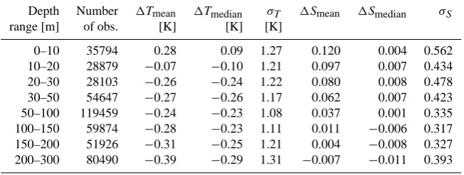
Table 1. Model temperature and salinity errors within Icelandic waters during the period 1992–2006 at the location and time of all available CTD profiles. Listed are the mean and the median model errors as well as the standard deviationσof the mean error.
Depth Number 1Tmean 1Tmedian σT 1Smean 1Smedian σS
range [m] of obs. [K] [K] [K]
0–10 35794 0.28 0.09 1.27 0.120 0.004 0.562 10–20 28879 −0.07 −0.10 1.21 0.097 0.007 0.434 20–30 28103 −0.26 −0.24 1.22 0.080 0.008 0.478 30–50 54647 −0.27 −0.26 1.17 0.062 0.007 0.423 50–100 119459 −0.24 −0.23 1.08 0.037 0.001 0.335 100–150 59874 −0.28 −0.23 1.11 0.011 −0.006 0.317 150–200 51926 −0.31 −0.25 1.21 0.004 −0.008 0.327 200–300 80490 −0.39 −0.29 1.31 −0.007 −0.011 0.393
data covered the period 1992–2006 and thus provided the temporal range of the ocean simulation.
Figure 3 shows the seasonal variation of the discharge and its spatial variation. Along the west coast, several water-sheds show higher mean winter values compared with sum-mer values due to higher precipitation in the winter months. However, most watersheds, and especially those being fed by glacier melt, e.g., at the south-east coast, show maximum values during late spring or summer.
3.2 Results and validation
In general, the model confirms the classic image of the circu-lation discussed above. The three-dimensional hydrography of Icelandic waters from 1992 to 2006 is well reproduced, including temporal anomalies, like the collapse of the NIIC during spring 1995 or its maximum in July 2003 (Jónsson and Valdimarsson, 2005). In order to monitor the model’s ability to simulate temporal variability we have compared the freely forecasted monthly temperature and salinity change in Icelandic waters with the monthly change computed includ-ing the data assimilation routine. Hence, the portion of freely forecast change should be close to 0 % if the model, just in-terpolating CTD profiles, were unable to reproduce any phys-ical process. However, the median portions are 91 % for tem-perature and 89 % for salinity.
In accordance with observations (Jónsson and Valdimarsson, 2004; Våge et al., 2011b) the model shows the NIJ as a deep undercurrent along the North Icelandic continental slope dominating the deep southward transport in northern Denmark Strait. The simulated NIIC volume flux is realistic, but it has been under-estimated by previous model versions, which led to several model experiments incorporating a manipulated wind field over Denmark Strait (Logemann et al., 2010). However, not wind stress changes but the assimilation of CTD profiles finally caused the decisive jump of the simulated NIIC volume flux. This was surprising considering our numerical experiments that investigated the role of local density gradients in Denmark
Strait in forcing the NIIC did not show clear results (see Sect. 4).
The simulated temperature and salinity fields of Icelandic waters are close to observations (Fig. 4), which is not sur-prising considering the assimilation of CTD data. However, there are still deviations between the measured and the mod-elled data which are primarily caused by the sparse temporal resolution of the data assimilation routine, which was called only once per simulated month, i.e., the simulated fields de-scribing the 15th of each month were corrected towards esti-mations based on all measurements made during this month. The model errors at the time and location of the CTD profiles are given in Table 1.
The simulated ocean currents are also in general agree-ment with observations. We compared the modelled flow field at the depth of 15 m with observations from a series of surface drifter experiments performed by Valdimarsson and Malmberg (1999). These include 19 GPS tracks of drift at the depth of around 15 m in Icelandic waters between May 1998 and December 1999. By using a low-pass filter to remove tidal and shorter periods, i.e., by computing the mean drift over time intervals of 60 h, 607 drift vectors were derived. These vectors were compared with their modelled counter-parts (Fig. 5).
This comparison of the flow velocity resulted in a me-dian (mean) model error of −0.64 cm s−1 (−1.22 cm s−1)
with a standard deviation of 6.54 cm s−1, whereas the
me-dian (mean) error of the modelled flow direction was 4◦(6◦) to the right with a standard deviation of 67◦. A former model version without CTD assimilation showed a median velocity error of−2.8 cm s−1(Logemann et al., 2010) which points to the improvement of the flow field simulation caused by the assimilation of CTD profiles.
938 K. Logemann et al.: The circulation of Icelandic waters
Fig. 4. Observed (left panels) and simulated (right panels) temperature (upper row) and salinity (lower row) in May 2003 at the depth of 50 m. Observational based charts are drawn after charts published by the Marine Research Institute, Iceland (www.hafro.is/Sjora/). The black dots show the location of CTD stations.
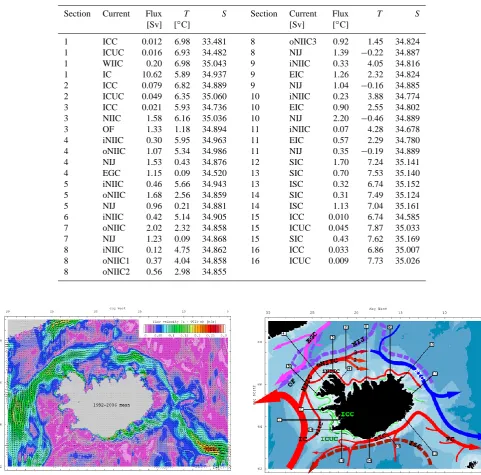
salinity in the core of the FC to be 8.08◦C and 35.24 during that period. Our simulated equivalents are 7.52◦C and 35.16. Figure 6 shows the simulated mean flow field around Ice-land at a depth of 15 m, averaged over the period 1992 to 2006. The striking features are the general eastward flow north and south-east of the island and the contrasting area of sluggish north-westerly flow in the south-west. Fig-ure 7 gives a schematic overview of the simulated three-dimensional circulation pattern, denotes different currents and defines 16 analysis sections. The current’s mean prop-erties across these sections – volume flux, temperature and salinity – are listed in Table 2.
The definitions of the currents revealed in this study (Fig. 7) are based upon the 1992–2006 mean flow field, i.e., we refer to the long-term mean dynamic structures and do not consider the water mass composition of the flow. These def-initions, comprised of positions and directions, were applied to the 12×15 monthly mean flow, temperature and salin-ity fields in order to obtain the values listed in Table 2. Oc-casionally, for reasons of clarity, hitherto unnamed currents are named, strictly following the existing naming system and without any pretence of final validity. In this way, we identi-fied the following currents in Icelandic waters.
Table 2. Simulated 1992–2006 mean volume flux, temperature and salinity of the currents in Icelandic waters across the 16 analysis sections. See Figure 7 for the locations of the sections and for the abbreviations of ocean current names.
Section Current Flux T S Section Current Flux T S
[Sv] [◦C] [Sv] [◦C]
1 ICC 0.012 6.98 33.481 8 oNIIC3 0.92 1.45 34.824 1 ICUC 0.016 6.93 34.482 8 NIJ 1.39 −0.22 34.887
1 WIIC 0.20 6.98 35.043 9 iNIIC 0.33 4.05 34.816
1 IC 10.62 5.89 34.937 9 EIC 1.26 2.32 34.824
2 ICC 0.079 6.82 34.889 9 NIJ 1.04 −0.16 34.885
2 ICUC 0.049 6.35 35.060 10 iNIIC 0.23 3.88 34.774
3 ICC 0.021 5.93 34.736 10 EIC 0.90 2.55 34.802
3 NIIC 1.58 6.16 35.036 10 NIJ 2.20 −0.46 34.889
3 OF 1.33 1.18 34.894 11 iNIIC 0.07 4.28 34.678
4 iNIIC 0.30 5.95 34.963 11 EIC 0.57 2.29 34.780
4 oNIIC 1.07 5.34 34.986 11 NIJ 0.35 −0.19 34.889
4 NIJ 1.53 0.43 34.876 12 SIC 1.70 7.24 35.141
4 EGC 1.15 0.09 34.520 13 SIC 0.70 7.53 35.140
5 iNIIC 0.46 5.66 34.943 13 ISC 0.32 6.74 35.152
5 oNIIC 1.68 2.56 34.859 14 SIC 0.31 7.49 35.124
5 NIJ 0.96 0.21 34.881 14 ISC 1.13 7.04 35.161
6 iNIIC 0.42 5.14 34.905 15 ICC 0.010 6.74 34.585 7 oNIIC 2.02 2.32 34.858 15 ICUC 0.045 7.87 35.033
7 NIJ 1.23 0.09 34.868 15 SIC 0.43 7.62 35.169
8 iNIIC 0.12 4.75 34.862 16 ICC 0.033 6.86 35.007 8 oNIIC1 0.37 4.04 34.858 16 ICUC 0.009 7.73 35.026 8 oNIIC2 0.56 2.98 34.855
Fig. 6. Simulated mean flow field around Iceland at 15 m depth, av-eraged over the period 1992 to 2006 and bottom topography (1500, 1000, 500 and 200 m isobaths).
3.2.1 Icelandic Coastal Current (ICC) and Icelandic Coastal Undercurrent (ICUC)
We define the ICC as a near-shore ocean current being driven by the barotropic pressure gradients due to a runoff in-duced coastal density reduction, therefore directed clockwise around the island. In order to analyse the spread of the coastal freshwater over the Icelandic waters, we computed the
sea-Fig. 7. Proposed three-dimensional circulation scheme of Icelandic waters with the locations of the 16 analysis sections. Dashed arrows denote deep currents. The abbreviations are: EGC – East Green-land Current, EIC – East IceGreen-landic Current, FC – Faroe Current, IC – Irminger Current, ICC – Icelandic Coastal Current, ICUC – Ice-landic Coastal Undercurrent, iNIIC – inner NIIC, ISC – IceIce-landic Slope Current, NIJ – North Icelandic Jet, NIIC – North Icelandic Irminger Current, OF – Overflow, oNIIC – outer NIIC, SIC – South Icelandic Current, WIIC – West Icelandic Irminger Current.
940 K. Logemann et al.: The circulation of Icelandic waters
Fig. 8. Mean simulated winter (left) and summer (right) freshwater thickness of Icelandic waters for the time period 1992 to 2006.
freshwater would form if it was separated from the seawater with which it is mixed. By constraining to the upper 300 m of the water column we used
hFW= z=0 m
Z
z=−300 m
SREF−S(z)
SREF
dz (4)
with the reference salinitySREF=35.2, which is assumed to
be the salinity of pure Atlantic Water. Figure 8 shows the re-sulting simulated mean winter and summer freshwater thick-ness fields around Iceland.
Given the seasonality of the discharge (Fig. 3) we find only little seasonal variation of the coastal freshwater thick-ness. Furthermore, only along the south-west and west coast a clear riverine, near-shore freshwater signal can be detected, whose northern parts are stronger in winter than in summer. Along the south-east coast, despite the great glacial discharge there, hardly any freshwater is found, not even during sum-mer, and along the north coast we see anhFW minimum in
contrast to the high values of the Arctic waters of the Iceland Sea north of it.
Therefore, within the 1992–2006 mean flow and salinity fields, we detected a clear ICC structure apart from several small-scale occurrences in bays and fjords only along the south-west and west coasts.
Originating north-east of the Westman Islands near the mouth of the Markarfljót River, the ICC is amplified between 50 and 100 km downstream by the discharge of the rivers Hólsá, Þjórsá and Ölfusá (see the row of four blue rectangles along the south-west coast in Fig. 3). With a volume flux usu-ally between 0.01 and 0.03 Sv the current follows the coast-line in a generally north-westerly direction towards Denmark Strait where it finally mixes into the NIIC (Fig. 7). Around the Snæfellsnes peninsula (eastern end of section 2) the ICC
Fig. 9. Simulated 1992–2006 mean of flow (positive (red) values denote northward flow), temperature and salinity across section 1 (eastern end). See Figure 6 for section location.
is exceptionally strong (0.08 Sv), broad and deep, pumping large amounts of freshened Faxaflói Bay water over the very steep topography to the north.
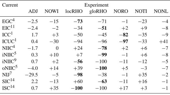
Table 3. Percentage change of the August to December 2003 mean volume flux of different currents (superscript number denotes the section) in the sensitivity experiments. Most notable changes are marked with bold numbers. The acronym ADJ denotes the model version with activated CTD data assimilation used for the long run. NIIC4denotes the sum of iNIIC4and oNIIC4. In case of experiment NORO only the December 2003 mean fluxes were considered.
Current Experiment
ADJ NOWI locRHO gloRHO NORO NOTI NONL
EGC4 −2.5 −15 −73 −71 −1 −23 −4
EIC11 −2.4 −2 −34 −51 +2 +9 −8
ICC1 1.7 +3 −50 −45 −82 −35 −9
ICUC1 0.4 −30 −94 −96 −97 −33 +41
NIIC4 −1.7 0 +24 −78 +2 +6 −7
iNIIC5 0.3 +10 +7 −99 −1 +6 −8
iNIIC9 0.7 +2 −56 −100 −11 −12 −5 oNIIC5 −4.0 +14 +39 −100 +5 −3 −7
NIJ7 −29.5 −5 −98 −38 −1 +35 −2
SIC14 2.2 −13 +60 −63 −11 +16 −1
ISC14 0.7 +35 −100 −100 +17 +3 −1
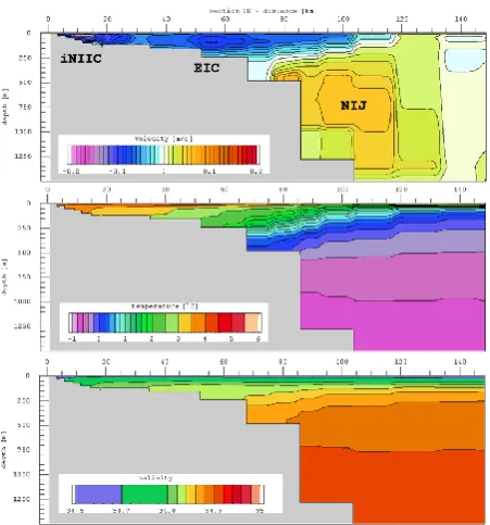
Fig. 10. Simulated 1992–2006 mean of flow (positive (red) values denote westward flow), temperature and salinity across section 5. See Fig. 6 for section location.
The simulated along-shore variability can be clearly seen by comparing the near-shore flow and salinity fields at sec-tion 1 (Fig. 9) and secsec-tion 5 (Fig. 10). Across secsec-tion 1 we see the ICC, associated with a sharp salinity increase from below 33 close to the coast to values above 34 20 km further offshore. However, at section 5 is coastal salinity gradient is smaller by one order of magnitude (from 34.8 at the coast to 34.9 20 km offshore) and the near-shore, wind-driven current is even directed westward, i.e., to the opposite direction of a potential freshwater driven coastal current.
With the exception of section 1 where the coastal pressure field is probably already dominated by the NIIC, we find the ICC being accompanied with a counter-directed undercurrent which we call the Icelandic Coastal Undercurrent (ICUC) (Figs. 7 and 9). This current has a volume flux comparable to that of the ICC but has a distinctly higher salinity. Its depth range is between 10 and 50 m and the width is around 10 km.
3.2.2 Irminger Current (IC) and West Icelandic Irminger Current (WIIC)
The IC is simulated to be the significantly strongest ocean current in Icelandic waters, flowing along the continental slope west of Iceland (Figs. 6 and 7). Originating along the western flank of the Reykjanes Ridge, the current transports 10.6 Sv of Atlantic and Subpolar Mode Water which is in good accordance with the Sarafanov et al. (2012) summer transport estimation of 12.0±3.0 Sv and below the value of 19±3 Sv given by Våge et al. (2011a). Between the con-tinental slope and the Icelandic coast, over the West Ice-landic shelf, we find an IC branch which is rather sluggish and broad and herein called the West Icelandic Irminger Cur-rent (WIIC) (Fig. 7). Note that in Fig. 7 the schematic source path of the WIIC contains a substantial cross-isobath com-ponent. Hence, the corresponding flow should not be under-stood as continuous and straight but, according to Valdimars-son (1998), rather as sluggish and eddy-induced. Figure 9 shows this current flowing across section 1 with its core close to the surface between 420 and 445 km. The WIIC originates over the continental slope north of the Reykjanes Ridge and flows northward over the western shelf until it finally joins the NIIC in Denmark Strait. The mean volume flux is 0.2 Sv, the temperature varies seasonally between 6 and 9◦C and the salinity is slightly above 35.
3.2.3 North Icelandic Irminger Current (NIIC), North Icelandic Jet (NIJ) and East Icelandic Current (EIC)
942 K. Logemann et al.: The circulation of Icelandic waters
Fig. 11. Simulated 1992–2006 mean of flow (positive (red) values denote north-westward flow), temperature and salinity across sec-tion 10. See Fig. 6 for secsec-tion locasec-tion.
off in Denmark Strait and flows northward along the Ice-landic shelf edge, which again is in agreement with obser-vations (Kristmannsson, 1998; Jónsson and Valdimarsson, 2005). This current absorbs the WIIC (≈0.2 Sv) in southern Denmark Strait. Shortly after crossing the Denmark Strait Sill, having lost around 0.2 Sv to the southwards flowing EGC, the NIIC splits into an inner (iNIIC≈0.3 Sv) and an outer branch (oNIIC≈1.1 Sv).
Whereas the iNIIC flows eastward along the North Ice-landic coast, the oNIIC takes an outer eastward route along the North Icelandic continental slope. The iNIIC can be traced downstream to the east coast of Iceland which is occa-sionally also reached by parts of the oNIIC. However, within the simulated long term mean, the oNIIC, after leaving Den-mark Strait where some mixing with the Polar Water of the EGC occurs, broadens and increases its volume flux by en-trainment of Arctic waters (1.1 Sv at section 4, 1.7 Sv at sec-tion 5, 2.0 Sv at secsec-tion 7). Before reaching the Kolbeinsey Ridge the oNIIC divides into three branches where the north-ernmost branch (≈0.9 Sv) with a mean temperature below 1◦C and a salinity close to 34.8 already shows more Arctic than Atlantic Water characteristics which may cast into doubt its denotation as an NIIC branch.
East of the Kolbeinsey Ridge the three oNIIC branches partly join the Arctic and Polar waters of the EIC which flows southward along the eastern flank of the ridge. Another in-terpretation of our model results would be to describe the EIC as a continuation of the oNIIC with some intrusion of Arctic and Polar waters flowing southwards along the
east-Fig. 12. Simulated 1992–2006 mean of flow (positive (red) values denote north-eastward flow), temperature and salinity across section 13. See Fig. 6 for section location.
ern flank of the ridge (Figs. 6 and 7). With a volume flux of around 1 Sv the EIC follows the continental slope to the east and continues along the northern flank of the Iceland–Faroe Ridge.
Below the EIC we find a counter-directed, cold (−0.5 to 0.4◦C) and salty (34.876 to 34.889) undercurrent; the NIJ (Figs. 7 and 11). Flowing westward along the continental slope at a depth between 200 and 1000 m, the current reaches a volume transport above 2 Sv east of the Kolbeinsey Ridge (section 10). After crossing the ridge the volume transport is reduced to 1.4 Sv (section 8) and continues to decrease as the flow is approaching northern Denmark Strait. However, through section 5 we still see an NIJ of 0.96 Sv with a temper-ature of 0.2◦C and a salinity of 34.881. Further downstream, across section 4, the NIJ is simulated to swell up to 1.53 Sv. Then, the NIJ opens out into the Denmark Strait Overflow (OF) a bottom-intensified and density-driven flow down the southern flank of the Greenland-Iceland sill forming a major part of the Meridional Overturning Circulation’s lower limb. The mean OF volume flux was simulated to be 1.33 Sv. 3.2.4 South Icelandic Current (SIC) and Icelandic Slope
Current (ISC)
Fig. 13. Time series (13-months moving average) of simulated and observed volume fluxes around Iceland and of the southward wind component (10 m height) north of Denmark Strait (black curve). Green: simulated North Icelandic Jet (NIJ) across section 5; red: simulated Atlantic Water (T >4.5◦C) transport of the North Ice-landic Irminger Current (NIIC) across section 5; light red dashed: Atlantic Water transport of the NIIC close to section 5 derived from current meter data (after Jónsson and Valdimarsson, 2012); blue: simulated South Icelandic Current (SIC) across section 13.
shelf at the southernmost tip of Iceland at around 19◦W: more than 20 cm s−1 averaged over the 1992–2006 period
(see Fig. 6). Here, the near surface core of the current is found less than 5 km south of the coastline. Like the WIIC the SIC is fed by the eddy-induced and sluggish northward flow of Atlantic Water south of Iceland which contains cross-isobath components shown schematically in Fig. 7. Further downstream the current flows further offshore and broad-ens as the shelf broadbroad-ens. Thereby additional Atlantic Wa-ter is entrained leading to an increasing SIC volume trans-port towards the east: 0.3 Sv at section 14, 0.7 Sv at section 13 and 1.7 Sv at section 12. The current is nearly unaffected by horizontal density gradients and therefore shows a homo-geneous velocity profile from the surface down to the sea floor (Fig. 12). Figure 12 also indicates that the SIC consists of an inner and an outer branch. Finally, having reached the Iceland–Faroe Ridge, the SIC turns to a south-easterly direc-tion, follows the ridge and opens out into the Faroe Current (FC). The FC volume flux north of the Faroe Islands was simulated to be 2.1 Sv. Hence, we conclude that 15, 33 and 81 % of its water stem from the SIC crossing section 14, 13 and 12, respectively.
Along the south-eastern continental slope of Iceland, at the depth between 500 and 1100 m, with the core at around 800 m, our model shows a topographically steered deep counter-current, herein called the Icelandic Slope Current (ISC) (Fig. 7). The ISC consists of re-circulating deeper At-lantic Water which explains the increase of its volume flux between section 13 (0.32 Sv) and section 14 (1.13 Sv).
3.2.5 Inter-annual variability of the NIIC, NIJ and SIC
Our results show that in 2003 the NIIC volume flux, in terms of the 13-months moving average, reached its absolute max-imum of the period from 1992 to 2006 (Fig. 13). We obtain the same result when expanding the period’s end from 2006 to 2010 by taking into account of the observational records of Jónsson and Valdimarsson (2012). A comparison of the modelled and observed NIIC is given in Fig. 13. Here, re-garding the time interval July 1995 to June 2006, the sim-ulated mean NIIC volume flux is 0.84 Sv whereas the ob-servational based equivalent is 0.85±0.13 Sv (Jónsson and Valdimarsson, 2012). Pearson’s correlation between the two time series is 0.77. Note that in Fig. 13, only the Atlantic Wa-ter content of the NIIC is considered which was computed with aT >4.5◦C criterion applied to the sum of the iNIIC and oNIIC crossing section 5. Our simulation shows an 85 % increase of the multi-annual mean NIIC; the simulated flux of Atlantic Water across section 5 was 0.54 Sv during the pe-riod 1992 to 1999 and rose to 1.00 Sv during 2001 to 2006.
The NIJ volume flux across section 5 shows a period of rather high transport, 1.03 Sv during 1992 to 1999, which is followed by a phase of weaker transport, 0.75 Sv during 2001 to 2006; a decrease of 27 %. Figure 13 also shows the devel-opment of the southward wind component north of Denmark Strait (at the position 67◦400N, 22◦320W where Logemann and Harms (2006) found a correlation of 0.857 between the meridional wind stress and the NIIC). We see a period of strong southward wind, strong NIJ and weak NIIC during 1997 to 2000. Afterwards these conditions are reversed.
The SIC across section 13 shows the same “remarkably stable” behaviour, at least between 1995 to 2002, as that of the FC analysed by Hansen et al. (2003). The SIC transport through section 13, which solely consists of Atlantic Water, was simulated to be 0.69 Sv during the period 1992 to 1999, clearly above the simulated NIIC Atlantic Water transport at that time.
4 Sensitivity experiments
In order to examine the forcing mechanism behind the dif-ferent simulated currents, a series of sensitivity experiments was carried out. First, the data assimilation routine was deac-tivated, the model was restarted at 12 July 2003 and a simu-lation until the end of 2003 was performed. This output, not disturbed by the corrections towards observations but fully consistent with the physical model equations, was used as the reference. A comparison of this solution with the orig-inal, including data assimilation, showed only minor devia-tions (experiment ADJ in Table 3) which ensures that the ref-erence run is still realistic with just the NIJ being intensified by 29.5 %.
944 K. Logemann et al.: The circulation of Icelandic waters
Fig. 14. Bathymetry and mean surface wind stress averaged over the period 1992 to 2006. In the frame of the various sensitivity ex-periments different forcing terms were switched off within the red encircled area.
sensitivity experiments. We decided on a circular area hav-ing its centre at 64◦360N, 20◦560W, a radius of 512 km and a transition ring with the width of 64 km at its boundary where the abnormal inner conditions were linearly led back to nor-mality (see Fig. 14).
The following six model runs, simulating the same time period as the reference run, were carried out:
1. NOWI – no wind stress in the local area
2. locRHO – no horizontal density gradients in the local area
3. gloRHO – no horizontal density gradients in the entire model domain
4. NORO – no Icelandic river runoff
5. NOTI – no tidal forcing in the entire model domain 6. NONL – no momentum advection in the entire model
domain
For each model run the August to December 2003 mean flow field and the corresponding difference of volume flux at each section relating to the reference run was computed. In the case of experiment NORO, because of the retention time of the freshwater within the coastal area, in order to obtain a maximum signal, we compared only the mean December flow fields.
The following interpretation of the six sensitivity exper-iments is based on the assumption that a significant reduc-tion of a current’s flow rate, caused by the deactivareduc-tion of a specific term, points towards an important role of the re-lated physical process in forcing the current. We have listed a selection of relative volume flux changes of the different currents within the different experiments in Table 3 where the most significant results are marked with bold numbers. These indicate that:
– None of the currents are primarily driven by the lo-cal wind stress. Figure 15d shows the wind stress im-pact on the flow field in the depth of 15 m. The main structure is a rather weak westward, near-shore flow north and south of Iceland, a westward flow in the Ice-land Sea and a south-westward EGC enforcing com-ponent along the East Greenland coast. Note that these results refer to the specific time period August to De-cember 2003. The wind field has a strong influence on the formation of the coastal freshwater induced salin-ity front which may explain the sensitive reaction of the ICUC, the reduction by 30 % at section 1, in exper-iment NOWI.
– The ICC and ICUC were reduced by 82 and 97 %, respectively in experiment NORO and hence are pri-marily driven by pressure gradients due to coastal den-sity reduction caused by river runoff. However, tide-induced residual currents and the wind stress are also important. Figure 16a and c show the dynamic effects of river runoff and tides, respectively. Whereas the tide-induced residual currents become relevant close to some headlands and along the south coast, counter-acting the SIC, the runoff-induced effects are very small along the southeast and northwest coast. How-ever, along the southwest and north coast a clear fresh-water signature is visible driving the ICC/ICUC and enforcing the iNIIC, respectively. Experiment locRHO (Fig. 16b) indicates that also the WIIC is related to coastal but further offshore density gradients.
– The EGC in Denmark Strait is mainly driven by barotropic pressure gradients related to the Polar Front. Deleting the local horizontal density gradients in experiment locRHO led to an EGC volume flux re-duction of 73 %. Figure 16b shows the dynamic im-pact of the local density field. Almost the entire EGC signal can be seen. Further forcing results from the tidal residual currents (23 %) and the local wind stress (15 %).
Fig. 15. Results of the sensitivity experiments gloRHO and NOWI. August 2003 to December 2003 mean flow fields at the depth of 15 m simulated by (a) the reference run and (b) the experiment gloRHO. (c) Shows the difference of both fields (gloRHO subtracted from the reference run). (d) Shows the results of experiment NOWI subtracted from the reference run.
the NIIC in Denmark Strait and of the SIC increased in experiment locRHO by 24 and 60 %, respectively, indicating that the local density field is not a critical factor of the basic NIIC/SIC structure.
– Not more than 10 % of the NIIC in Denmark Strait can be explained by the inertia of the IC along its curved path south of the strait. The NIIC reduction in experi-ment NONL varies between 5 and 8 % (Fig. 16d). – The NIIC and SIC are predominantly driven by the
barotropic pressure field related to the Arctic Front. This last conclusion was drawn when observing the im-mediate shutdown of the currents when horizontal density gradients were removed from the entire model domain (ex-periment gloRHO), whereas both currents increased when only the local density gradients were removed (experiment locRHO). Hence, our sensitivity experiments pointed to-wards the basin-scale pressure field, i.e., the difference of the sea surface height between the colder and denser waters to
the north and the warmer waters to the south of Iceland, be-ing the main forcbe-ing factor of the currents. In order to further illuminate this point an additional model experiment was car-ried out.
4.1 NIIC/SIC forcing experiment
In order to understand the nature of the NIIC and SIC forcing, we set up a very simple hydrodynamic scenario:
– a rectangular ocean basin at the reference latitude of 65◦N with closed boundaries and side lengths of 1600×1600 km;
– an undisturbed ocean depth of 3000 m and a circular island of the radius of 210 km in the centre of the basin described by
D(r)=500 m
1−tan h
1.0472×10⁻⁵m−1r−π
, (5)
946 K. Logemann et al.: The circulation of Icelandic waters
Fig. 16. Results of the sensitivity experiments NORO, locRHO, NOTI and NONL. Simulated mean flow fields at the depth of 15 m subtracted from those of the reference run. Difference vector fields relating to (a) December 2003 mean of experiment NORO, (b), (c) and (d) August 2003 to December 2003 means of experiments locRHO, NOTI and NONL, respectively. Note that the results of experiment locRHO are only relevant within the local area (Fig. 14).
– a zonal, stationary density front separating denser wa-ter with 1028.4 kg m−3 in the north from less dense water with 1027.9 kg m−3 in the south, roughly de-scribing the conditions around Iceland. The meridional density profile is given by
ρ(y)=1027.9 kg m−3+0.25 kg m−3
1+tanh
y−800 km 30 km
, (6)
withybeing the meridional distance from the southern boundary (see Fig. 17a).
The solution of this problem was determined with a sim-plified version of the CODE model, using a homogenous horizontal grid with a spacing of 10 km and 37 z levels with a vertical spacing from 10 m near the sea surface to 160 m close to the sea floor. Using a time step of 30 s the model was spun up by linearly raising the density gradi-ents from zero to the prescribed values during the first sim-ulated week. The density gradients caused hydrostatic pres-sure gradients. These caused a southward flow which raised the sea level south of the front until the related near-surface northward flow balanced the southward. Quasi-stationary, mainly geostrophic conditions were achieved shortly after-wards (Fig. 17b–d).
Figure 17b shows the difference of sea surface height be-tween the northern (lower level) and southern (higher level) part of the basin due to the density difference. Like the density the sea surface height forms a front which is, dis-tant from the island, on top of and parallel to the density front. The resulting pressure gradient force leads to an upper layer geostrophic eastward flow along the front (Fig. 17c). A counter-current is found in deeper layers (Fig. 17d).
However, close to the island, this structure is distorted. When hitting the island, the upper eastward flow causes a zone of high pressure at the island’s western (windward) coast and a low pressure zone at the eastern (lee side) coast. These pressure anomalies spread along the coast in the Kelvin wave propagation direction. The consequences are two geostrophic northward currents along the west and the east coast, extending to the north and south coast, respec-tively. These two currents have a clear similarity to the NIIC and SIC.
Fig. 17. Setup and results of the NIIC/SIC forcing experiment. (a) Topography and prescribed stationary density field, (b) stationary sea surface elevation after the spin-up, (c) stationary flow field at the depth of 45 m, (d) stationary flow field at the depth of 2500 m.
in the first case and its amplification in the second, show that a shelf, i.e. a sufficiently broad coastal area with sig-nificantly reduced water depth, is a prerequisite of the NIIC/SIC structure.
5 Discussion and conclusions
In this paper we have analysed a hydrodynamic simulation of Icelandic waters covering the time period 1992 to 2006. Thereby, we have concentrated particularly on the tempo-ral mean state derived from the model output. However, we also presented the simulated temporal variability of the in-volved ocean currents which partly contains considerable inter-annual fluctuations. Furthermore, we know that the re-gional marine climate occasionally has undergone dramatic changes (Malmberg and Kristmannsson, 1992). Hence, this paper should not be understood as an attempt to specify
ever-fitting structures of a stationary system, but rather as a pro-posed description of the current state.
948 K. Logemann et al.: The circulation of Icelandic waters
Fig. 18. Results of the NIIC/SIC forcing experiment performed with two different topographies. Stationary solutions after the spin-up are shown. (a) The topography without a shelf, (b) the resulting sea surface elevation, (c) the resulting flow field at the depth of 45 m, (d) the topography with a wide shelf, (e) the resulting sea surface elevation, and (f) the 45 m flow field for this case.
north-eastward boundary current of Atlantic Water not only erodes the coastal freshwater signature but also counteracts the development of a south-westward flow.
Hence, our model results offer a solution to the ICC quandary, which is defined by two opposing schemes of the coastal circulation around Iceland: (a) the classical view of a freshwater-induced current flowing clockwise around the island (e.g., Stefánsson and Ólafsson, 1991; Halldórsdóttir, 2006); and (b) the assumption that freshwater-induced near-shore dynamics do not form a separate current, with the coastal circulation instead thought to derive from the off-shoots of the larger ocean currents further off-shore (e.g., Astþórsson et al., 2007). Our findings point to the possi-bility that both views are correct when applied to different coastal sections. They illustrate the transport of freshwater along the south-west coast in accordance with the measure-ments of Stefánsson and Guðmundsson (1978) and Ólaf-sson et al. (1985, 2008), but also explain the sparse oc-currence of polar driftwood at south-eastern beaches which is in sharp contrast to the large deposits often found at north-eastern beaches (Eggertsson, 1994) – an observation that indicates the absence of a steady southward current connecting these areas.
Another result of this study is the possible existence of an undercurrent below the ICC, which we have called the
Ice-landic Coastal Under-Current (ICUC). Unfortunately there are no long-term current measurements from the depth range within the shallow near-shore waters along the south-west coast where we predict the ICUC to occur. We are there-fore unable to confirm or refute our model predictions; how-ever, the simulated structure is compatible with the theoret-ical predictions of ocean physics. These predict a counter-directed undercurrent if an along-shore density front exists which reaches down to the bottom-boundary layer (Chapman and Lentz, 1994; Pickart, 2000).
Fig. 19. Different interpretations of the Atlantic Water flow (red or black arrows) between Iceland and the Faroe Islands: (a) from Ste-fánsson and Ólafsson (1991), (b) from Valdimarsson and Malmberg (1999) based on drifter data, (c) the classical view of Atlantic Water pathways (unbroken arrows) and “alternative suggestions” (broken arrows) from Hansen et al. (2003), (d) the Atlantic Water pathways suggested by Orvik and Niiler (2002) based on drifter data. Modi-fied after Stefánsson and Ólafsson (1991), Valdimarsson and Malm-berg (1999), Orvik and Niiler (2002), and Hansen et al. (2003).
meaningful (below the ICC) and not along the entire resolu-tion boundary.
The theory of secondary circulation related to Ekman-layer dynamics (e.g. Holton, 1979; MacCready and Rhines, 1993) says that a system consisting of an along-shore density front, a coastal current in the Kelvin wave propagation direc-tion and a counter-directed undercurrent implies upwelling within the density front. Such an upwelling could play an important role for the Icelandic ecosystem by carrying nu-trients from the bottom layer up to the euphotic zone where the primary production is intensive (Ólafsson et al., 2008). This could be, in addition to the river-borne silicate, an-other cause of the higher phytoplankton productivity over the south-western shelf compared to that of the adjacent open sea as observed by Guðmundsson (1998).
Along with the ICC and ICUC, our focus was on the ma-jor currents in Icelandic waters, which mostly flow further offshore over the shelf or along the continental slope, their long-term mean spatial structures and the underlying forcing mechanisms. In order to analyse the forcing of the different currents, a set of numerical sensitivity experiments was car-ried out, whereby each experiment dealt with one specific physical forcing process.
The basis for these experiments was the assumption that the volume flux of a simulated current would collapse in a short period of time in the case that its relevant forcing process would have been deactivated within the model equa-tions. Whereas this chain of thought is self-evident in the ma-jority of the experiments, the situation becomes more
com-plex in the case of experiment locRHO and gloRHO. Here, we are faced with the problem that, e.g. a wind-driven current in a stratified ocean will lead to horizontal density gradients which could be misinterpreted as forcing the current. How-ever, deleting the horizontal density gradients from the model equations, like we did in experiments locRHO and gloRHO, would change the simulated vertical shear of the wind-driven current but it would not lead to a collapse of its volume trans-port. This collapse would happen only after the wind stress terms were deleted. When analysing the six sensitivity ex-periments we focussed on the vertically integrated flow, i.e. the volume transport, and thereby circumvent this problem of misinterpretation. It should be also noted that we ask for the immediate regional forcing, e.g. the pressure field result-ing from sea level height gradients across the Arctic Front if the according geostrophic flow substantially corresponds to the analysed current and if a removal of this pressure field leads to a collapse of the current. However, we would like to stress here that the Arctic Front in turn is formed by struc-tures like the basin-scale wind field, the meridional gradient of the ocean–atmosphere heat flux and the topography of the Greenland–Iceland–Scotland Ridge separating the different water masses.
One important result regarding the near-surface major cur-rents is the general dominance of an eastward flow around Iceland caused by the different sea level height between the Atlantic Water to the south and the Arctic waters to the north. Two almost symmetric branches, the NIIC to the north and a current of similar strength herein called the South Icelandic
Current (SIC) to the south carrying Atlantic Water along the
north-western and south-eastern side of the island, respec-tively. Both currents are found to be forced by barotropic pressure gradients which form as a result of the Arctic Front’s pressure field interacting with the topography of the Icelandic shelf (see Figs. 17b and 20). Though the local wind and the local baroclinic pressure gradient cause temporal variability of these currents, they are not their primary forcing. This in-dependence of the coastal circulation on wind forcing is sup-ported by the results of the numerical sensitivity experiments performed by Ólason (2006). Furthermore, our findings are in agreement with recent works on the forcing of the Faroe Current (FC) (Hansen et al., 2010; Richter et al., 2012; Sandø et al., 2012). Herein, the meridional gradient of sea surface height across the Arctic Front, caused by the density gradi-ent or even by the removal of dense water by the overflow (Hansen et al., 2010), is identified as the basic forcing of the FC. Therefore, the assumption of an analogous forcing of the SIC and NIIC appears to hold true.
950 K. Logemann et al.: The circulation of Icelandic waters
Fig. 20. Left: the simulated 1992–2006 mean sea surface elevation around Iceland. Right: the mean dynamic topography model of Huneg-naw et al. (2009) calculated from marine, airborne and satellite gravimetry, combined with satellite altimetry. Modified after HunegHuneg-naw et al. (2009).
finally mixes into the Arctic waters of the East Icelandic Cur-rent (EIC) which flows southward along the eastern flank of the ridge. Note that, beside its temporal variability, the simu-lated shape of the oNIIC branching may also strongly depend on the vertical topography resolution which is, far away from the coast, only 160 m.
The NIIC is the result of the signal of high dynamic sea level height south of Iceland which is led downstream along the west and north-west coasts. An analogous structure is found along the east and south-east coasts where the signal of low dynamic sea level height from north of Iceland is led southwards and upstream (Fig. 20). But how are these signals led? Is it possible that the Arctic Front density gradient off the east (west) coast forces a barotropic current up to 300 km further up-(down)-stream off the south (north) coast?
This problem was first examined by Csanady (1978) who discussed solutions of the stationary, linearised and depth-averaged equations of motion along an idealised coastal slope adjoining a deep sea area. His theory treats a coastal pressure and according flow signal which extends, from the region where an along slope sea surface gradient is imposed at the shelf break by a deep water dynamics, longshore in the direction of topographic wave propagation. Csanady de-noted the structure as an “arrested topographic wave”. Huth-nance (1987) has analysed the corresponding flow adjust-ment on the shelf. He describes the evolution of a barotropic alongshore flow (even for baroclinic forcing). The distance and the direction over which this evolution takes place shows a close correspondence to the decay distance and direction of the lowest mode continental shelf wave which is in the order of 1000 km. Huthnance points towards the clear decoupling of the coastal and the oceanic sea level in the case of an ar-rested topographic wave.
Over the south-eastern shelf the result of this effect is the SIC, simulated to flow with high intensity over the south-ern and south-eastsouth-ern shelf to the east and north-east, respec-tively. Our simulation showed months with the SIC being stronger than the NIIC or EIC, and indicated that the SIC is a substantial source of the FC, and could even be interpreted as the FC preform.
We successfully reproduced the NIIC/SIC structure and showed its dependency on the topography and the density field with an idealised model setup: a circular island be-ing placed on a zonal density front. This experiment resem-bles those of Hsieh and Gill (1984) addressing the Rossby adjustment problem (Rossby, 1937, 1938). Considering a meridional channel with a zonal density front Hsieh and Gill pointed to the existence of a northward western boundary current south of the density front and a northward eastern boundary current north of it, both being accompanied by deep counter-currents. They also discussed the application of their results to the hydrography of the Iceland–Faroe Ridge and, regarding their deep counter-currents, may have already shown the basic NIJ forcing mechanism.
However, are our model predictions of the SIC realistic? After all, a description of a specific eastward current over the southern and south-eastern Icelandic shelf, independent and separated from the North Atlantic Drift, does not exist within the classical view of Icelandic hydrography.