www.atmos-meas-tech.net/9/793/2016/ doi:10.5194/amt-9-793-2016
© Author(s) 2016. CC Attribution 3.0 License.
Global cloud top height retrieval using SCIAMACHY limb spectra:
model studies and first results
Kai-Uwe Eichmann1, Luca Lelli1, Christian von Savigny2, Harjinder Sembhi3, and John P. Burrows1 1Institute of Environmental Physics, University of Bremen, Bremen, Germany
2Institute of Physics, Ernst Moritz Arndt University of Greifswald, Greifswald, Germany 3Earth Observation Science, University of Leicester, Leicester, UK
Correspondence to: Kai-Uwe Eichmann ([email protected])
Received: 5 May 2015 – Published in Atmos. Meas. Tech. Discuss.: 10 August 2015 Revised: 8 January 2016 – Accepted: 8 February 2016 – Published: 2 March 2016
Abstract. Cloud top heights (CTHs) are retrieved for the pe-riod 1 January 2003 to 7 April 2012 using height-resolved limb spectra measured with the SCanning Imaging Absorp-tion SpectroMeter for Atmospheric CHartographY (SCIA-MACHY) on board ENVISAT (ENVIronmental SATellite). In this study, we present the retrieval code SCODA (SCIA-MACHY cloud detection algorithm) based on a colour index method and test the accuracy of the retrieved CTHs in com-parison to other methods.
Sensitivity studies using the radiative transfer model SCIATRAN show that the method is capable of detecting cloud tops down to about 5 km and very thin cirrus clouds up to the tropopause. Volcanic particles can be detected that oc-casionally reach the lower stratosphere. Upper tropospheric ice clouds are observable for a nadir cloud optical thickness (COT)≥0.01, which is in the subvisual range. This detection sensitivity decreases towards the lowermost troposphere. The COT detection limit for a water cloud top height of 5 km is roughly 0.1. This value is much lower than thresholds re-ported for passive cloud detection methods in nadir-viewing direction. Low clouds at 2 to 3 km can only be retrieved un-der very clean atmospheric conditions, as light scattering of aerosol particles interferes with the cloud particle scattering. We compare co-located SCIAMACHY limb and nadir cloud parameters that are retrieved with the Semi-Analytical CloUd Retrieval Algorithm (SACURA). Only opaque clouds (τN,c>5) are detected with the nadir passive retrieval tech-nique in the UV–visible and infrared wavelength ranges. Thus, due to the frequent occurrence of thin clouds and sub-visual cirrus clouds in the tropics, larger CTH deviations are detected between both viewing geometries. Zonal mean CTH
differences can be as high as 4 km in the tropics. The agree-ment in global cloud fields is sufficiently good. However, the land–sea contrast, as seen in nadir cloud occurrence fre-quency distributions, is not observed in limb geometry. Co-located cloud top height measurements of the limb-viewing Michelson Interferometer for Passive Atmospheric Sound-ing (MIPAS) on ENVISAT are compared for the period from January 2008 to March 2012. The global CTH agreement of about 1 km is observed, which is smaller than the vertical field of view of both instruments.
1 Introduction
Clouds are extremely variable in form and size in the Earth’s atmosphere. Thus the physical cloud parameters, for exam-ple the optical thickness, albedo, and the bottom/top heights from near the ground up to the tropopause, are highly vari-able. Clouds cover about 66 % of the Earth. The value de-pends on the used optical thickness threshold (Stubenrauch et al., 2013). Clouds are composed of liquid particles (T >
0◦C), ice (T ≈<−38◦C), or a mixed phase for intermediate temperatures (Boucher et al., 2013).
Clouds also impact the Earth’s radiative balance and play a major, yet still relatively uncertain, role in the changing en-ergy budget (IPCC, 2013). The overall cloud radiative effect depends on cloud type and top height, which is a combina-tion of greenhouse warming (longwave) and reflective cool-ing (shortwave). The knowledge of global cloud characteris-tics is essential in different fields of numerical analyses, for instance, weather prediction, circulation, or climate change models.
Optically thick clouds scatter a high percentage of the in-coming visible light back to space due to their high albedo. A cloud radiative effect of about−50 Wm−2is expected due to the enhancement of the annual global albedo. Additionally, clouds absorb and emit infrared (terrestrial) radiation, which strongly depends on cloud temperature. The longwave effect is annually and globally averaged on the order of 30 Wm−2 (Boucher et al., 2013). Cloud properties and their develop-ment in a changing climate will determine the net effect.
The light scattering ability of cloud droplets in the visi-ble and near infrared is only weakly wavelength dependent in comparison to light scattered by molecules. Furthermore, light inside a cloud will encounter enhanced path lengths as it is scattered multiple times at the water or ice particles inside the cloud, and light absorption by trace gases in the clouds will be enhanced.
Tropical clouds can reach heights of roughly 17 km. Either deep convective clouds or the more common cirrus clouds are observed in the tropical tropopause layer (TTL) above 14 km (Fueglistaler et al., 2009). Cirrus clouds are mainly formed in the upper troposphere (above 8 km) by condensation nuclei such as mineral dust and metallic particles via heterogeneous freezing. Larger biological particles are removed by deposi-tion before reaching these altitudes. Cirrus clouds are either produced by the uplift of humid air or by a convective blow-off from deep convection. They are made of small ice crys-tals due to the low temperatures at these heights (<−30◦C)
(Cziczo et al., 2013).
In 84 % of the measurements of Cloud–Aerosol Lidar and Infrared Pathfinder Satellite Observations (CALIPSO), cirrus layers have a vertical extension of less than 1.5 km at heights between 13 and 16 km (Massie et al., 2007). Only 1.5 % of the cirrus are more than 3 km thick. Cirrus layers near the tropopause can be as thin as 0.5 km and have a horizontal extent up to a few thousand kilometres as detected by
Li-dar measurements made on the space shuttle (Winker et al., 1998).
Cirrus clouds are categorized as (a) subvisual, i.e. optically very thin with cloud optical depths (COD) τN<0.03, (b) thin (0.03< τN<0.3), or (c) opaque (τN>0.3) (Sassen and Cho, 1992). Subvisual clouds are mainly found in the tropics with higher occurrence frequencies over oceans and during the night. Thin cirrus clouds are more frequent at night and are found mainly over equatorial land masses and the west-ern Pacific. Moreover, opaque cirrus clouds are mainly found during the day over oceans (Sassen et al., 2009). Cirrus cloud occurrence frequencies (COFs) are also coupled to the dy-namic circulation patterns. Davis et al. (2013) reported that TTL thin cirrus COFs are partly driven by the quasi-biennial oscillation (QBO) and the upwelling in the tropical branch of the Brewer–Dobson circulation (BDC). For example, a re-duced BDC upwelling and a warm QBO westerly phase in-crease the TTL temperature and reduce the relative humidity, which in turn leads to a COF reduction.
High-altitude, optically thin clouds are nearly transparent for the incoming shortwave solar radiation, but they partially absorb Earth’s outgoing longwave radiation. As the cloud particles are much colder than the surface, they re-emit com-paratively less radiation towards space. The net effect is a warming of the atmosphere below the cloud (“cloud green-house forcing”). Low clouds (zct<3 km), however, are the main contributors to an enhancement of the global albedo. Leahy et al. (2012) found that nearly half of all clouds over non-polar oceans have low top heights ofzct<3 km. These clouds have an horizontal extent on the order of 2 km. Approximatively 40 % of all clouds are low-level (above 680 hPa, below 3.2 km), 15 % are mid-level, and 45 % high-level (below 440 hPa, above 6.5 km) clouds (IPCC, 2013).
A number of satellite missions are specially designed for the detection of cloud properties. For example, CALIOP uses the laser wavelengths of 532 and 1064 nm to measure phys-ical cloud tops with high accuracy of about 60 m in the tro-posphere (Winker et al., 2009). Thin clouds with an optical thickness of about 0.01 are still detectable with this tech-nique. Stubenrauch et al. (2013) reported an average global cloud amount of about 68 % for clouds with optical depths higher than 0.1. This increases to 73 % when also taking the subvisible cirrus clouds into account (Winker et al., 2009; Chepfer et al., 2010).
Optically thin clouds can also be observed by passive sensors in limb or occultation geometry. For instance, the Stratospheric Aerosol Gas Experiment II (SAGE) instrument aboard the NASA Earth Radiation Budget Satellite (Wang et al., 1996) was able to detect very thin clouds with COD
τN>0.03. SAGE detected a high global cloud amount of 95 % (Stubenrauch et al., 2012). A long light path of about 200 km around the tangent point increases the number of pos-sible cloud measurements. The Optical Spectrograph and In-frared Imaging System (OSIRIS) on-board Odin is a limb-viewing instrument that can accurately measure thin cirrus top heights and COF above 12 km using the 1530 nm IR channel (Bourassa et al., 2005) and the optical thickness of subvisual cirrus clouds at 750 nm (Normand et al., 2013). The High Resolution Dynamics Limb Sounder (HIRDLS) on-board the AURA spacecraft detects cirrus clouds, deep convective clouds, and polar stratospheric clouds (PSCs) using infrared radiances at 12.1 µm (Massie et al., 2007). Michelson Interferometer for Passive Atmospheric Sound-ing (MIPAS) on ENVISAT detected similar cloud parame-ters using bands in the mid-wavelength infrared and thermal infrared regions (Spang et al., 2012; Sembhi et al., 2012).
Clouds in the instruments’ field of view influence the retrieval accuracy of atmospheric trace gas concentrations from limb measurements. The cloud-contaminated part of the measurement profile should be omitted in the retrieval algorithm to minimize trace gas retrieval errors (Sonkaew et al., 2009). As a consequence, we have developed the SCIA-MACHY cloud detection algorithm (SCODA). This retrieval scheme uses a colour ratio method to detect cloud top heights in limb-viewing geometry. It was implemented in the SCIA-MACHY level 2 operational processor (version 5.04) (ESA, 2013) to improve the limb trace gas retrievals towards the tro-posphere. It is also used for scientific profile retrievals of up-per tropospheric/lower stratospheric water vapour and trace gases like nitrogen dioxide, bromine oxide, and tropospheric ozone (Rozanov et al., 2011; Weigel et al., 2016; Ebojie et al., 2014).
In this study limb observations from the SCIAMACHY spectrometer are used to retrieve cloud top heights using the SCODA colour index ratio approach. We investigate the sen-sitivity of the method to detect clouds in limb view for dif-ferent tropospheric cloud types using the radiative transfer model SCIATRAN. We study the latitudinal and seasonal
variations of cloud heights. Optically thin clouds throughout the free troposphere were detected and even very thin vol-canic aerosol layers in the upper troposphere/lower strato-sphere (UT/LS) region. Height-resolved cloud occurrence frequencies are derived from the cloud top height data set to study global cloud field distributions. The method is verified by comparing to other satellite data and literature.
The paper is structured as follows. Section 2 provides information on the data used for this study. The retrieval method to compute cloud top heights from the limb-scattered profiles is described in Sect. 3. The influence of the limb path and the instrument’s vertical field of view on the results is analysed in Sect. 3.1. Section 4 presents model simulations performed with the radiative transfer model SCIATRAN to investigate the robustness of the method. SCIAMACHY re-trieval results are discussed in Sect. 5. The rere-trieval method is validated with SCIAMACHY nadir data and MIPAS limb data in Sect. 6. Section 7 explains the influence of volcanic aerosols on retrieval results and conclusions are given in Sect. 8.
2 Data
2.1 SCIAMACHY
The atmospheric science instrument SCIAMACHY on board of ESA’s ENVISAT is a high-resolution eight channel grat-ing spectrograph (Burrows et al., 1995; Bovensmann et al., 1999). ENVISAT was launched on 1 March 2002 into a po-lar, sun-synchronous orbit with a mean local Equator cross-ing time of 10:00 at the descendcross-ing node. Contact to the satellite was lost on 8 April 2012. The SCIAMACHY instru-ment covered a spectral range from the UV-C (214 nm) to the near-infrared IR-B (2386 nm), with a channel-dependent spectral resolution between 0.22 and 1.48 nm. Scattered, re-flected, transmitted, and emitted electromagnetic radiation was observed in solar/lunar occultation, nadir-, and limb-viewing geometry. More details can be found in Gottwald and Bovensmann (2011).
2.1.1 Limb data
The focus of the SCIAMACHY limb observations are the re-trieval of stratospheric O3, NO3, and BrO profiles using day-time measurements of scattered solar radiation (see Gottwald and Bovensmann (2011) and references therein). Further-more, polar stratospheric cloud top heights and stratospheric aerosol extinction profiles are detectable and mesospheric temperatures are retrieved using night-time limb measure-ments.
Figure 1. The Earth’s limb as seen from the International Space
Station on 16 June 2010. The ISS nadir point is in the Aegean Sea at 36.8◦N latitude and 27.1◦E longitude. Image courtesy of the Im-age Science & Analysis Laboratory, NASA Johnson Space Center, Mission-Roll-Frame ISS024-E-6137 (http://eol.jsc.nasa.gov).
ground and a change of colour near the surface from dark blue to light blue/white, where we expect the influence of clouds.
SCIAMACHY’s instantaneous field of view was at the tangent point 2.6 km (vertical field of view, VFOV) in ver-tical and 110 km in horizontal direction (across-track) for the nominal limb-scatter mode. The scanning time of each tan-gent height was 1.5 s. Typically four distinct measurements were made in across-track direction from west to east. Each measurement had a horizontal resolution of 240 km due to the scanning speed and integration time (Bovensmann et al., 1999) and a total swath of 960 km. The horizon was scanned in vertical direction from below the ground to about 92 km tangent height in more than 30 steps that are 3.3 km apart (Gottwald and Bovensmann, 2011). This measurement cycle is called a limb state. A profile was not fully vertical due to the movement of the satellite and the scanning scheme. The maximum horizontal displacement between all tangent height points within one profile was about 60 km in the tro-posphere. The atmosphere was undersampled with a ver-tical gap of roughly 0.7 km between two adjacent tangent heights. The along-track horizontal resolution was approx-imately 410 km for one VFOV shell. The limb horizontal resolution is analysed in Appendix A. Full coverage of the Earth required 6 days at the Equator with faster coverage to-wards the polar regions. Figure 2 shows a schematic view of the limb geometry. The red solid line depicts the instruments line of sight (LOS) and the field of view (FOV) as red dot-ted lines. The blue circles depict the tangent heights for each LOS, which are numbered from the bottom to the tropopause. We used the SCIAMACHY version 7.04W level 1b spec-tra. The level 1b data were calibrated without the polar-ization correction due to known problems in limb geome-try (Liebing, 2013). The radiometric calibration was
omit-Figure 2. Schematic view of the limb measurement geometry. The
shells are numbered from the surface to the tropopause (here 1 to 6). The field of view (FOV), the tangent height step width1zth, and the cloud top heightzct are superimposed. Examples of shell path lengthsxas blue lines and areasa(grey shaded) are shown. The limb path is a combination of the paths through each shell. The sub-pathsx(3,3)andx(3,4)(blue line) are depicted belonging to shell 3. The first index stands for the original tangent height and the second index for the current shell of the path segment.
ted as the colour index ratio is a division of two neighbour-ing tangent height measurements and thus no absolute cal-ibration was needed. Height-resolved limb-scattered spectra were taken from the instrument channels 4 (750 nm) and 6a (1090 nm). These wavelengths were chosen to avoid molec-ular absorption bands, e.g. for ozone, oxygen, and water vapour. The retrieval would be disturbed because of the addi-tional absorption features with different height distributions. Radiation at wavelengths below 400 nm is not suitable be-cause the atmosphere gets optically thick in the upper tropo-sphere due to Rayleigh scattering and ozone absorption in-creases towards the Hartley–Huggins bands (von Savigny et al., 2005b).
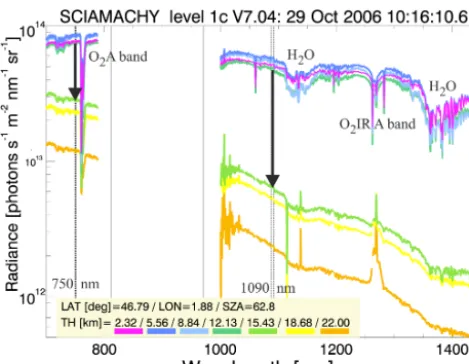
Figure 3 displays the limb radiances I (pho-tons s−1m−2nm−1sr−1) of channels 4 and 6 as a function of wavelengthλ (nm) for tangent heights ranging from 2.3 to 22 km. Radiances from channel 5 are not plotted. High intensities are detected for the four lowest tangent heights, where the slope between the retrieval wavelength bands is low. At the tangent height of 15.4 km, the intensities drop significantly compared to 12.1 km and a steeper gradient between both bands is measured (see black arrows). We conclude that a cloud layer is in the field of view at the lower tangent height. A larger quantity of radiance is scattered into the line of sight. Furthermore, the intensity decreases less with increasing wavelength due to the particle scattering. 2.1.2 Tangent height knowledge
Figure 3. SCIAMACHY limb radiances from channels 4 (700–
789 nm) and 6 (1000–1300 nm) for tangent heights (TH) from 2.3 (violet) to 22.0 km (orange). A measurement sequence of the EN-VISAT orbit 24382 (AZM 1) from 29 October 2006 (measurement start time 10:16:10.62 UTC) at 46.8◦latitude, 1.9◦longitude, and 62.8◦sun zenith angle from operational level 1c data version 7.04W (calibration parameters 0–5) has been used. The cloud retrieval wavelength bands around 750 and 1090 nm are shown as vertical dashed-dotted black lines and the channel borders as grey lines. The largest intensity decrease in both bands is marked by the black ar-rows.
real tangent height have reached several kilometres (Kaiser et al., 2004; von Savigny et al., 2005a). The main reasons for the tangent height differences are satellite attitude knowledge errors and a misalignment between the SCIAMACHY opti-cal axes and the satellite reference frame, which were later identified and corrected (Gottwald et al., 2007). The geomet-ric tangent height knowledge of the operational level 1 ver-sion 7 limb data is now accurate within 170 m (Gottwald et al., 2010; Bramstedt et al., 2012).
Mean SCIAMACHY limb tangent heights from azimuth index 3 (eastern profile) and the corresponding 2σ standard deviations (blue dashed) are calculated from the first mea-surements of each orbit per day at the beginning of each month (Fig. 4). Superimposed is the difference between two adjacent tangent heights (red line), which is ≈3.3 km. At the beginning of the mission in 2003 we detect the largest intra-annual variations when tangent heights varied between 6.8 km in spring and 4.7 km at the end of the year. The limb measurement cycle was optimized at this time. The intra-annual amplitude was about 150 m until the end of the year 2010 with lowest tangent heights at the beginning of each year. In October 2010, the orbital height of the EN-VISAT satellite has been lowered by about 17.4 km to ex-tend the mission lifetime. As a consequence, each limb state was truncated by one tangent height step to maintain the limb/nadir matching (Gottwald and Bovensmann, 2011; Ebo-jie et al., 2014). The limb tangent height pattern was
modi-Figure 4. Time series of one limb tangent height (in km) covering
the SCIAMACHY mission lifetime; e.g. TH(3) is the tangent height with index number 3. Daily means were plotted, taken from the first state of 10 orbits of 1 day per month (usually the first day). The dashed blue lines depict the corresponding 2σ standard deviation. The red line shows the tangent height step width, which is here the difference TH(4)–TH(3) between two adjacent tangent heights.
fied again in January 2011 (see also Fig. 4) when tangent heights were lowered by roughly 100 m and the step width was slightly reduced.
2.1.3 Nadir data
SACURA (Rozanov et al., 2004; Kokhanovsky et al., 2005) retrieves the effective radius of cloud droplets, the liquid water path, and other parameters like the optical thickness for optically thick clouds (τN≥5). The cloud top height is determined from spectral measurements in the oxygen A band (755–770 nm). The total cloud top height error is about ±400 m for most of the cases (Lelli et al., 2012) (Fig. 1). However, it increases with cloud height and can be up to 1400 m for high clouds with a low optical thick-ness. SACURA takes multiple scattering of light inside and below the clouds into account (Lelli, 2013). Therefore, the SACURA model is more accurate than retrieval schemes treating clouds as Lambertian reflectors. Stubenrauch et al. (2012) showed that passive remote sensing techniques tend to detect a “radiometric cloud top height”, which can be up to a few kilometres lower than the physical cloud top height. We used SACURA cloud top heights retrieved with SCIA-MACHY level 1 version 7.04W data.
2.2 MIPAS
spec-tral resolution (Fischer et al., 2008). While SCIAMACHY scanned the limb in forward flying direction of the ENVISAT satellite, MIPAS faced backwards. MIPAS had a similar res-olution as SCIAMACHY in limb mode along the LOS and in vertical direction (3 km). However, the resolution perpen-dicular to the LOS of 30 km was considerably higher than SCIAMACHY (240 km). Due to the specific spectral mea-surement range, MIPAS was able to measure day and night and as a pure limb sounder recorded more limb scans per orbit than SCIAMACHY.
The MIPAS scan measurement time in nominal mode was 56.7 s with 27 floating altitude grid points from 7 to 72 km after 2005. After severe in-flight anomalies in 2004, the duty cycle of 100 % was reached again in December 2007. The vertical sampling step size in the UT/LS region was 1.5 km, which led to an oversampling of the atmosphere by a factor of 2. SCIAMACHY instead undersampled the atmosphere. The lowest tangent height was not constant along the orbit. It varied from 5 km at the poles to 12 km at the Equator as a function of latitudeφwithzth(φ)=12−7∗cos(90−abs(φ)) (Raspollini and Ceccherini, 2011). Thus only cloud top heights above 8.5 km were retrieved in the tropics and ex-tratropics (30◦N/S).
Different methods to detect clouds have been adopted for MIPAS (Spang et al., 2012). Using a cloud index (CI) method (Spang et al., 2002), a fast detection scheme for the op-erational level 2 processing was developed to omit cloud-contaminated measurements. This method was also used to derive cloud field characteristics like global cloud top dis-tributions and occurrence frequencies (Spang et al., 2005; Sembhi et al., 2012). The standard operational CI approach used two micro windows from 788.2 to 796.2 cm−1and from 832.0 to 834.4 cm−1in the MIPAS CI-A band with a fixed threshold (see Spang et al. (2012) and reference therein).
Sembhi et al. (2012) presented an optimized cloud and aerosol detection method for MIPAS in which new seasonal-, latitude-, and altitude-dependent cloud detection thresholds were calculated to maximize the sensitivity to cloud/aerosol particles in the MIPAS field of view. Based on these thresh-olds, a MIPAS CTH data set was calculated for the entire MIPAS mission. We use this data set from 2008 to 2012 for the study.
3 Determination of colour index ratios and retrieval of cloud top heights
SCIAMACHY provides measurements of the limb-scattered light integrated along the line of sight. Choosing only wave-lengths where trace gas absorptions and emissions can be neglected, for instance around 750 and 1090 nm, the de-tected radiation is dominated by the scattering processes of molecules, aerosols, and cloud particles (von Savigny et al., 2005b). Rayleigh theory describes scattering on air molecules, which is strongly wavelength dependent.
Scatter-ing on aerosols and cloud particles, however, is only weakly wavelength dependent and can be approximated by Mie the-ory. Water and ice clouds show similar scattering character-istics for the chosen wavelengths. Only above 1400 nm, the water and ice absorption have different and non-negligible spectral dependencies (Kokhanovsky et al., 2006), which can be used to discriminate phases or to distinguish between cloud and aerosol particle.
Dividing the spectrally averaged radiances of two wave-length bands (750–751, 1088–1092 nm) by each other, we can differentiate between measurements where particles are situated in the FOV and those not affected by particles. This is called the colour index approach. Colour is defined here as the ratio between radiances from two different wavelength bands of the same viewing LOS or tangent height. The tech-nique was previously applied to SCIAMACHY limb mea-surements for the detection of polar stratospheric clouds (von Savigny et al., 2005b) and the determination of the cloud top height of a hurricane cell (Kokhanovsky et al., 2005). This work is a generalization of these previous studies with respect to global particle (cloud) detection and the use of SCIAMACHY tangent heights from the Earth’s surface up to 30 km.
The cloud top heightzct (km) is determined using radi-ance profiles in different wavelength regions. The height-dependent colour index CI(zth)is first calculated for all tan-gent heightszth [km] from the ratio of two limb-scattered radiance intensitiesI at different wavelengthsλ:
CI(zth)=
Ih(zth, λh) Il(zth, λl)
, (1)
where h denotes the high and l the low wavelength band. The radiances are spectrally averaged for the two bands 750 to 751 nm (l) and 1088 to 1092 nm (h). The signal-to-noise ra-tios of SCIAMACHY are roughly 2000 at 15 km tangent height (Bovensmann et al., 1999) for both the low and the high band, so that noisy spectra have a negligible effect on the retrievals in general. The colour index ratio (CIR)2[−] can then be defined as
2(zth)=
CI(zth) CI(zth+1zth)
, (2)
where1zthis the step width between two adjacent tangent heightszth,i andzth,i+1. The tangent height grid of SCIA-MACHY limb observations, for example the spacing be-tween two adjacent altitude levels, is about 3.3 km wide. This also determines the retrieval accuracy. The step width (Fig. 4, red line) is rather constant throughout the mission lifetime.
The function2(zth)peaks at the tangent height where the cloud top zct is within the field of view along the line of sight. SCIAMACHY has undersampled the atmosphere in limb view. Cloud tops up to 0.6 km above the FOV are thus not detectable at the next higher tangent height.
Figure 5. Normalized colour index (a) and colour index ratio (b) of
a SCIAMACHY limb state (see Fig. 3) for tangent heights from the ground to 30 km. All four limb profiles (AZM 0–3) are measured simultaneously during a limb state. Superimposed is a cloud-free limb profile (red line) from the same orbit (start time 10:38:59 UTC, AZM 3). The green dashed line depicts the cloud detection thresh-old.
chosen to reduce false detections due to aerosols in the lower troposphere (see Sect. 4). von Savigny et al. (2005b) used 1.3 for the detection of lower stratospheric PSCs. A radiance calibration is not necessary due to the use of ratios, where all multiplicative and height-independent errors cancel out. However, additive errors such as stray light can still influence the retrieval results (Langowski et al., 2015).
Figure 5 shows the retrieved profiles of (a) the cloud colour index and (b) the colour index ratio for a SCIAMACHY limb state (29 October 2006, 10:16:10.63 UTC) over Europe with four independent profiles in across-track direction of the flight path. For visualization purposes the colour index is nor-malized by the highest tangent height. A sharp CI decrease at 12 km is visible for all four measurements. Superimposed is a cloud-free profile (red line) from the same orbit, which ex-hibits a low surface CI value and a slow decrease with height. Clouds are detected when the CIR2peak exceeds the thresh-old of 1.4 (dashed green line). Depending on the atmospheric conditions,2(zth)is an unknown function of the cloud op-tical thickness (COT), scattering geometry, albedo, aerosol loading, and signal-to-noise ratio of the measurements. The sensitivity of2to the scattering geometry and optical char-acteristics will be discussed in Sect. 4.
2(zth)can peak more than once in a vertical profile, but only the highest cloud top detected is stored with a corrected quality flag. The double peaks occur in roughly 10 % of all retrievals, suggesting that two or more distinct cloud layers are detected. This happens when, for example, a high thin cloud lies above a low thick cloud. It is not possible to sepa-rate the cloud layers when the highest cloud is optically thick. The limb-viewing geometry is not well suited to deal with
layered clouds as the position of a cloud along the light path is not known (see also Appendix A).
3.1 Limb optical thickness
The main difference between nadir and limb cloud detection is the much larger limb path length and the much coarser hor-izontal resolution. Long pathways greatly enhance the sensi-tivity of the limb measurements. However, looking sideways into a cloud field leads to a loss of information on the cloud amount at the tangent point. Thus retrieved cloud occurrence frequencies will in general be much higher than what is de-tected in nadir geometry. This will be further analysed in Sect. 5.
The cloud optical thicknessτLin limb-viewing geometry is larger than the vertical optical thicknessτNdue to the long horizontal light path. The path length depends on the instru-ment’s VFOV and the tangent height. For example, an en-hancement factor of 226 for the limb optical depth is calcu-lated for a cloud field covering the full VFOV of 1 km and a top at 15 km tangent height. Due to the curvature of the at-mosphere, a cloud layer drops below the VFOV at a specific point along the line of sight. Taking the area defined by the lines of the VFOV that intersect a shell into account, we cal-culate an area weighted enhancement factor (AWF) of 151.
This is the highest possible enhancement, because a cloud is not a horizontal layer and will not cover the VFOV com-pletely. The AWF for the SCIAMACHY VFOV of 2.6 km is 243. This factor is generally too high. For example, thin cirrus clouds will only fill a part of the VFOV. We simulate this effect by reducing the VFOV to 0.1 km and then get an AWF≈47. This is a more realistic value for the increase of the vertical optical depth in limb geometry.
As a result, a subvisual cloud layer with an optical thick-ness τN=0.01 lying within the field of view of SCIA-MACHY has a limb τL of about 2.4 (AWF=243) and roughly 0.5 for vertically thin clouds (AWF=47). In limb view, clouds are detected against the surrounding atmosphere and the background space. The contrast between a cloudy and non-cloudy part of the profile is high compared to a nadir scene. The air pressure above a cloud is lower, less scatter-ing occurs, and the air mass appears darker. The decrease of brightness towards outer space is also visible in Fig. 1. The nadir cloud detection is partly dependent on the contrast at the ground. For instance, ice and snow lead to larger errors in the cloud optical thickness determination (Lelli et al., 2012; Lelli, 2013).
4 Model simulations
Table 1. Pairs of corresponding latitude, longitude, sun zenith angle
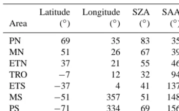
(SZA), and relative sun azimuth angle (SAA) of one tangent point in SCIAMACHY limb measurement geometry (PN: polar north, MN: midlatitude north, ETN: extra-tropical north, TRO: tropics, MS: midlatitude south, PS: polar south, ETS: extra-tropical south). A measurement from ENVISAT orbit 24381 from 29 October 2006 for the (western) azimuth index 0 is taken for this example.
Latitude Longitude SZA SAA Area (◦) (◦) (◦) (◦) PN 69 35 83 35 MN 51 26 67 39 ETN 37 21 55 46 TRO −7 12 32 94 ETS −37 4 41 137 MS −51 357 51 148 PS −71 334 69 156
physical properties (optical thickness, effective radius of par-ticles, phase function, cloud phase). This is of course a strong simplification of the complex 3-D structure of a cloud, which cannot be resolved with these kind of models.
The software package SCIATRAN version 3.1.28 (Rozanov et al., 2014) is used to study the strengths and lim-itations of the fast and simple CIR retrieval method. The CIR sensitivity is tested for typical atmospheric cloud scenarios like low optically thick or high subvisible clouds. Therefore the influence of cloud parameters (for example, optical thickness τ, top height, layer thickness) and geolocation (sun zenith angle, sun azimuth angle) on the colour index ratio is investigated. The forward model includes a cloud model and has been described and validated by Rozanov et al. (2014). The radiance accuracy is generally better than 1 % compared to other radiative transfer models.
ENVISAT moved from the north to south along the orbit on the day side, with varying sun zenith angle (SZA) and relative sun azimuth angle (SAA) combinations at the limb tangent point. Because of the sun-synchronous orbit with a descending node crossing time of 10:00, only certain com-binations of these parameters were possible. The largest sun zenith angles were found near the poles and minima in the tropics (about 26◦). The relative azimuth angle was gener-ally lower towards the northern high latitudes (SAA about 22◦) and largest at southern high latitudes (SAA about 157◦). Light scattering on aerosols and cloud particles is largest in the north due to stronger forward scattering at low az-imuth angles. Minimum scattering occurs in tropical regions for SAAs around 90◦. Table 1 shows typical combinations of the SCIAMACHY limb measurement geometry for different latitudes of orbit 24381 from 29 October 2006.
The following parameters are chosen for the tests of CIR sensitivity in a cloudy atmosphere for different cloud top/bottom heights, optical thickness, and geometry. A spher-ical atmosphere with refraction is modelled with the
radia-tive transfer model SCIATRAN (Rozanov et al., 2014). The scalar discrete ordinate technique is used to solve the radia-tive transfer equation, where absorption of the trace gases O3, NO2, and SO2is taken into account. The surface is modelled as a Lambertian reflector with a constant albedo as=0.1, which is roughly twice as high as the albedo of water sur-faces. The tangent heights are placed from 0 to 30 km with a step width of 3 km. Radiances are modelled for the wave-lengths 750.0 to 751.0 nm with 0.2 nm step width and 1088.0 to 1092.0 nm with 0.8 nm step width, corresponding to the SCIAMACHY channels 4 and 6. The SZA varies between 20 and 82◦and the SAA between 20 and 160◦to cover the range of values of the SCIAMACHY limb measurements (see Ta-ble 1).
We simulated limb radiances for four typical cloud scenar-ios to find the limitations of the cloud retrieval method with respect to cloud height and optical thickness. The maximum colour index ratios for one retrieval height are shown as func-tion of sun azimuth and sun zenith angles in Fig. 6. Two wa-ter cloud layers with (a) the vertical extents of 2–3 km (low-est cloud case) and (b) 5–6 km (general water cloud case) are modelled. The spectrally dependent optical thicknesses are τN,wc=10.0 and 0.1 at 500 nm respectively. Two cir-rus cloud layers made of hexagonal ice crystals with 100 µm height and 50 µm side length (Rozanov et al., 2014) are sim-ulated. We assume (c) an optical thicknessτN,ic=1.0 for the layer 8–10 km (general ice cloud case) and (d) 0.01 for 14– 15 km (subvisual ice cloud case).
The value of CIR is mainly driven by geometry, retrieval height, and cloud and aerosol optical thickness. Thus, we choose combinations of rather low COTs and high aerosol optical thicknesses (AOTs) for all cases except (a). The ef-fective radius of the water droplets is 10 µm (Rozanov et al., 2014), which is in the range of values from literature (Rossow and Schiffer, 1999). The particle size has a negli-gible effect on the CIR of less than 1 % when varying, for instance, the water droplet size between 10 and 50 µm. In general, ice crystals can vary substantially in size from about 10 to 2000 µm and exhibit a variety of different shapes (Liou, 2005). However, the CIR is not sensitive to the size of the ice crystals. The CIR varies by less than 1 % when the crystal size is doubled.
calcu-Figure 6. Simulated colour index ratios as a function of sun zenith angle and sun azimuth angle for different cloud layer heights. The
radiances are calculated using the SCIATRAN forward model. The CIR are retrieved on a 3 km height grid. The black and white dots depict zenith and azimuth angle pairs for a typical SCIAMACHY orbit. Small azimuth angles correspond to the Northern Hemisphere and large values to the Southern Hemisphere. Please note the different colour scales for water and ice clouds.
lated using the single parameter Henyey–Greenstein analyti-cal formula with an asymmetry factor of 0.772 (0.0–4.0 km), 0.669 (4.0–10.0 km), and 0.657 (above 10.0 km) (Rozanov et al., 2014). The AOT defined at 790 nm corresponds to a larger AOT at 550 nm. For example,τN,a=0.25 at 790 nm is roughly equal to 0.4 at 550 nm.
The step size for the calculations is 5◦ in SZA and 10◦ in SAA direction. The black dots depict tangent point SAA/SZA combinations along a typical SCIAMACHY orbit for the west and east profiles with azimuth angle index 0 and 3. Cloud tops are in general detectable for all SZA/SAA pairs for a CIR threshold of 1.4. When the retrieved cloud height differs from the simulated one, the CIR is not plotted (white areas).
In panel (a) we simulate a low, thick water cloud (2–3 km,
τN,wc=10.0) in a clean area (τN,a=0.07), which is found mostly over the oceans (Remer et al., 2008). Cloud tops are detected at 3 km tangent height for most of the geometry combinations except for high SZA. If the modelled aerosol loading is set to the global oceanic mean of 0.14, CTHs at 3 km would not be detectable anymore. Because most of the aerosol particles are in the lower layer with an optical depth of roughly 0.125 between the ground and 5 km, the CIR is reduced and the retrieved CTH shifted to the next retrieval tangent height of 6 km.
Low CIR values near the threshold are calculated in side-ways (tropics) and backward direction (southern high lati-tudes) of the scattered light beam (panel b). The cloud is be-tween 4 and 5 km with low COTτN,ic=0.1 and an oceanic global meanτN,a=0.14. High CIR values are found where the water droplet phase function has a peak in forward di-rection. The CIR of a simulated cloud increases when the cloud is shifted upwards in the model. Thus the threshold is mainly chosen to sort out wrong cloud top heights due to high aerosol loadings in the lower altitudes. Cloud tops are cor-rectly retrieved above 5 km for moderate AOTτN,a≤0.14. Clouds at the lowest possible SCIAMACHY tangent height between 2 and 3 km are only retrievable for very low aerosol loading (τN,a≤0.07). The lowest AOTs are found in clean areas over oceans, especially in the Southern Hemisphere.
The water phase function has a relatively broad minimum around 100◦. This explains the CIR difference for water (a,
b) and ice (c, d) particles between 60 and 120◦, where CIR is
more sensitive to ice particles. High CIRs are found for large SAA/SZA values, making the method also very sensitive to polar stratospheric clouds as already shown by von Savigny et al. (2005b).
The strong CIR dependence on tangent height is already observable in Fig. 6 (Fig. S1 in the Supplement). For in-stance, the retrieved CIR nearly doubles from about 1.6 (TH=5 km) to 3.1 (TH=18 km) when moving a water cloud (τN,wc=1.0) with a vertical thickness of 1 km through the troposphere. The retrieval sensitivity is high enough at lower tangent heights. Under normal aerosol conditions (AOT<0.14) clouds are detectable for COTs τN,wc≥0.1 at 6 km retrieval height and τN,wc≥0.005 in the upper troposphere at 15 km. Sub-visible ice clouds in the upper troposphere are already detectable for cloud optical thick-nesses τN,ic≥0.003 (SZA=25◦, SAA=83◦, cloud layer 15–16 km). The influence of background aerosols and refrac-tive tangent height changes are negligible at these heights. However, the cloud retrieval can occasionally be obstructed by enhanced levels of aerosols from volcanic activity in the upper troposphere when optical thicknesses of clouds and aerosols have the same order of magnitude. The COT lim-its have been calculated for a spherical shell cloud layer and have to be interpreted as theoretical lower limits. In reality, we expect lower CIR values for very thin cirrus cloud fields that have limited vertical and horizontal extents.
The SCIAMACHY level 1C tangent heights are geomet-ric ones where refraction is not taken into account. The real tangent height is lowered due to atmospheric refraction. The effect is negligible above 22 km, where differences between geometric and refracted tangent heights are less than 100 m. However, the light path at zth=6 km has a refracted tan-gent height of about 4.9 km. Furthermore, the vertical field of view increases. For the geometric VFOV, we calculate the lower edge at 4.7 km and the upper edge at 7.3 km. The corre-sponding refracted VFOV edges are 3.4 and 6.4 km respec-tively. The refractive VFOV is thus about 3 km wide. The lower VFOV edge at the geometric tangent height 2.3 km above the ground already is below the surface. Thus it is pos-sible to detect clouds down to the Earth’s sea surface. How-ever, the colour index ratio at the lowest heights is already near the threshold and the CIR is very sensitive to aerosol contaminations, which increase towards the surface.
5 Retrieval results
SCIATRAN was already used for cloud sensitivity studies on the limb ozone retrieval. Sonkaew et al. (2009) concluded that only tangent heights above the cloud top should be used for ozone profile retrievals in order to reduce ozone retrieval errors. The same limb measurement mode was used here to
derive cloud top heights in order to minimize differences in time and geolocation with respect to trace gas profile re-trievals. The cloud top height retrieval model SCODA was developed and then implemented in October 2010 into the SCIAMACHY level 2 version 5 operational processor (ESA, 2013) to support the retrieval of trace gas profiles in limb view.
SCODA retrieval results are presented in this chapter. We calculated annual means of cloud top heights and height-dependent occurrence frequencies for the troposphere. The limb COF is defined as the number of measurements flagged as cloudy within one grid cell and atmospheric layer divided by the number of all measurements for that grid cell. 5.1 Annually averaged cloud top heights and
occurrence frequencies
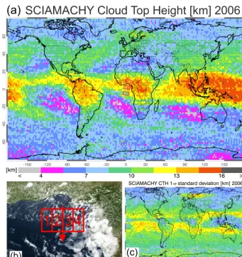
Figure 7a shows the annual mean cloud top height (km) for 2006. It is calculated by binning the cloudy measure-ments (roughly 445 000) on a 2◦×2◦map. Superimposed is the size and horizontal distance of about 780 km for three SCIAMACHY limb scan cycles or states (red rectangles). Each state is composed of four simultaneous measurements in across-track direction. The approximate footprint size of a limb state is superimposed in panel (b) to a cloud image from SEVIRI (Spinning Enhanced Visible and Infrared Im-ager) on-board the geostationary Meteosat Second Genera-tion (Schmetz et al., 2002). The lower left corner of the image is at the Equator over the Gulf of Guinea. The fine horizon-tal structure of a nadir cloud field is not detectable in limb view, because a large air volume is scanned in limb and only the highest cloud tops contribute to the measurement of that volume. Panel (c) shows the corresponding 1σ CTH stan-dard deviation. The largest scatter was found in tropical re-gions where the high cloud systems have a seasonal variation changing in north/south direction.
The highest cloud tops with heights of about 13 to 16 km are observed in the tropics. These are typically deep convec-tive and cirrus clouds. The lowest clouds are found in the Southern Hemisphere west of the continents (about 4 km). Also a stream of relatively high clouds is detected ranging from the Caribbean Sea over the northern Atlantic Ocean to-wards northern Europe, which can be related to extra-tropical storm tracks. Similar features are observed east of Japan and in the southern Pacific Ocean towards the west coast of South America. An interhemispheric CTH difference towards the poles is observed that will be further elucidated in Sect. 5.2.
Figure 7. Global map of (a) the annual mean cloud top height (in km) for 2006. The data are binned in boxes of 2◦latitude and 2◦longitude. The superimposed red rectangles show the approximate size of three consecutive SCIAMACHY limb scans. The SEVIRI image in (b) shows a part of the African continent near the Equator to illustrate the coverage of a cloud field in limb. It was provided by M. Reuter (Reuter and Pfeifer, 2011). The superimposed red rectangles give the sizes of the four limb measurements of one SCIAMACHY limb scan (limb state) at the tangent point. The arrow indicates the viewing direction. The annual mean CTH standard deviation (in kilometres) for 2006 is shown in (c).
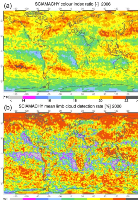
changes from 30◦(NH) to 150◦(SH) at latitudes where CIR differences are also found in our model studies (see Fig. 6a). Low CIR regions are furthermore detected in the low cloud top height areas, which is in line with our expectations from model studies. Panel (b) of Fig. 8 shows the SCIAMACHY limb cloud detection rate. A measurement flagged as cloudy is counted when the cloud top height is between 0 and 20 km. Very high values are detected in comparison to cloud occurrence frequencies retrieved in nadir geometry. More than 93 % of the 391 700 measurements made in 2006 are marked as cloudy. Cloud-free areas are only rarely detected in SCIAMACHY limb measurements because of the long tropospheric geometric path length of 1200 km. Spang et al. (2012) called it the “limb-smearing effect”, which makes comparisons to nadir measurements complicated. Compara-tively low cloud detection rates of about 70 % are found only
in low cloud top regions, west of the continental coasts in the Southern Hemisphere. The difference between both polar re-gions already seen in other CTH/CIR maps is also detected here.
Figure 8. Global annual mean of (a) the maximum colour index
ratio and (b) the limb cloud detection rate for 2006. The CIR is multiplied by a factor of 10.
5.2 Height-resolved cloud occurrence frequencies Figure 9 shows annual mean limb COF (%) for the year 2006. The COFs are calculated for six altitude layers. Each layer represents a SCIAMACHY tangent height, which was nearly constant over time and orbital position. The COF is calcu-lated by comparing the number of cloud detections in one layer and grid box with the number of all measurements of that grid box.
In layer 1.0–3.75 km (panel a) the largest amount of clouds are detected over oceanic regions in the Southern Hemi-sphere westwards of the continents. Slightly more clouds are observed between 1.0 and 6.5 km in the southern polar regions than in the northern counterpart. It seems that the method is rather insensitive to low clouds for small scatter-ing angles and large sun zenith angles, which are typical for high northern latitudes. Stray light might also be a factor that has to be further analysed. Furthermore, the limb-smearing effect can lead to higher retrieved CTHs.
The enhanced COFs over North Africa can be attributed to aerosols uplifted by dust storms over the Sahara, as this
region is nearly cloud free. Higher COFs were also de-tected over the African continent and west of it at the height range 3.75–6.5 km (b). CALIOP measured dust plumes from Africa up to 8 km altitude over the Atlantic (Generoso et al., 2008; Liu et al., 2008).
High COF between the midlatitudes and the polar re-gions were also detected by CALIOP (Chepfer et al., 2010) (see Fig. 3g–h). High COFs at low altitudes (CTH<3 km,
>680 hPa) were mainly found over the oceans, especially near the west coasts of the continents, which is in line with our observations from Fig. 9a. However, CALIOP observed no enhanced COFs over North Africa, supporting the argu-ment that SCIAMACHY detected an aerosol layer in this re-gion.
The largest interhemispheric COF differences are discov-ered in the layer 6.5–10.0 km shown in panel (c). The north-ern hemispheric COF at latitudes north of 60◦N is above
50 % and in the corresponding Southern Hemisphere on the order of 40 %. The combination of COF patterns of layers (a) and (c) explain the interhemispheric CTH differences as seen in Fig. 7. Langowski et al. (2015) observed that the first measurements of the sunlit part in the Northern Hemisphere are influenced by stray light and have to be excluded. For this reason only limb states of the descending orbit phase are used and also the first five states after the descend are omitted.
Cloud tops between 10 and 13.5 km are mainly detected in areas of frequent storm activities in the extra-tropical zone for latitudes higher than 30◦N/S (see Atlas of Extrat-ropical Storm Tracks http://data.giss.nasa.gov/stormtracks/). CALIOP also observed high level clouds above 7.2 km in these regions (Chepfer et al., 2010) (Fig. 3c–d).
The occurrence of clouds above 13.5 km is limited to the tropical zone as seen in panels (e) and (f). Largest COFs of about 70 % are detected over the western part of the Pacific from Indonesia to the east between 90 and 180◦ longitude. High clouds are also observed over Central Africa and Mid-dle America (above 40 %). Another feature is the slightly enhanced COF over Antarctica, which can be attributed to PSCs in the southern hemispheric winter/spring period from mid-June to early November.
5.3 Temporal evolution of CIR and CTH
Figure 9. SCIAMACHY annual mean cloud occurrence frequencies for 2006 and for tangent heights between (a) 1.0 and 3.75 km, (b) 3.75
and 6.5 km, (c) 6.5 and 10.0 km, (d) 10.0 and 13.5 km, (e) 13.5 and 16.5 km, and (f) 16.5 and 19.9 km.
Two other wavelength pairs are also tested for their temporal behaviour. Similar features are found for the 1551/1090 nm CIR, which is used in the limb water vapour retrievals as an additional constraint (Weigel et al., 2016). The CIR is also reduced dur-ing the longer instrument decontamination phases in August/December 2003, June/December 2004, and De-cember 2008. The 1685/1551 nm CIR is currently under study, which can possibly discriminate between clouds and aerosols. This ratio is rather stable for the whole period, indicating that it is insensitive to aerosols. If the CIR decrease is due to instrumental degradation, it could reduce the detection sensitivity for very thin cirrus and low-altitude clouds because of the constant detection threshold. Never-theless, the mean CIR is still well above 1.8 at the end of the instruments lifetime in 2012.
Time series of the SCIAMACHY CTH zonal monthly mean for latitudes between±75◦show an annual cycle and an interhemispheric CTH difference (Fig. 11a). High CTHs
Figure 10. Global monthly averages of the SCIAMACHY colour
index ratio CIR for the 1090/750 nm wavelength pair and its 1σ standard deviation. Also plotted are two different CIRs using the ratios of 1551/1090 nm (blue dashed line) and 1685/1551 nm (red dashed line).
Tavurvur (4◦S, 152◦E), which erupted between August 2006 and January 2007 with a Volcanic Explosivity Index of 4. Sulfur dioxide and ash clouds reached the tropopause in October 2006 and spread afterwards northwest and south-east (Global Volcanism Program, 2006). However, the largest CTHs and a large longitudinal scatter are observed at the end of 2011 in the latitude band 0 to 10◦N. Mean CTHs up to 21.3±8.2 km are detected in December 2011, while normal values are on the order of 13±4 km at this location and time of the year. So far the reason for this phenomenon is unclear and has to be further analysed. It might be attributed to rising aerosol particles after the Nabro eruption.
6 Validation with SCIAMACHY nadir and MIPAS limb cloud top heights
The comparison of limb measurements with nadir retrieved cloud parameters is no simple task due to long light paths as discussed in Sect. 4 and also addressed by Spang et al. (2012). We first compare cloud top heights retrieved from the two viewing geometries nadir/limb of SCIAMACHY and interpret the differences. We then validate our results with collocated limb CTH from MIPAS in the second subsection. 6.1 Comparison with SCIAMACHY nadir cloud
measurements
A perfect agreement between limb and nadir cloud top mea-surements cannot be expected. The two main limiting fac-tors are the low limb horizontal resolution and the high op-tical thickness threshold necessary for nadir retrievals using passive instruments like SCIAMACHY. We used SACURA data where the following quality checks were applied to
Figure 11. Time series of SCIAMACHY monthly zonal means
CTHs (a) and (b) 1σ standard deviations (in kilometres) for the period from January 2003 to April 2012 between 75◦S and 75◦N. The red dots depict the start dates and latitudes of 4 major volcanic eruptions: Kasatochi in August 2008, Sarychev Peak in June 2009, and both Nabro and Puyehue–Cordón Caulle in June 2011.
constrain the nadir data (see Lelli et al. (2012), Table 4): top height convergence (flag 2), top/bottom height conver-gence (5), high geometrical thickness (3), and a cloud optical thickness larger than 30.
0 20 40 60 80 (a) 1.0-3.75 km
0 20 40 60 80
(b) 3.75-6.50 km
0 20 40 60 80
(c) 6.50-10.0 km
0 20 40 60 80
(d) 10.0-13.5 km
0 20 40 60 80
(e) 13.5-16.5 km
0 20 40 60 80
(e) 13.5-16.5 km
0 20 40 60 80
(f) 16.5-19.9 km
[%] SACURA nadir cloud occurrence frequency year 2006
Figure 12. SCIAMACHY SACURA nadir cloud occurrence for the
year 2006, projected on a grid of 2◦-sided cells. From (a) to (f) val-ues are sorted in altitude layers as in Fig. 9. Due to the inherent conceptual difference between limb and nadir observation geom-etry, the occurrence is calculated averaging the actual nadir cloud fraction over time, resorting to the ergodic assumption by which space and time averages are equivalent.
CALIOP detected very thin clouds. For instance, 56 % of the total cirrus clouds are observed at subtropical latitudes of±30◦(Sassen et al., 2009).
The COFs for very low clouds over the oceans are en-hanced (>50 %) in both viewing geometries (a). The limb COF asymmetry between the polar Northern and the South-ern hemispheres especially in the lower layer (a) is not observed in nadir view. High nadir COFs are detected in the Northern Hemisphere over land (panel a–b) and over ocean (c). Contrarily, limb COFs are highest between 6.5 and 10 km north of 60◦N/S. These high clouds restrain the de-tection of low clouds in limb view. The enhanced limb COFs over North Africa due to aerosols are not observed in nadir data.
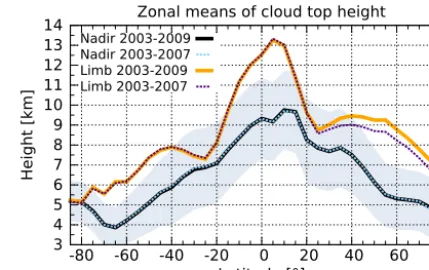
Figure 13 summarizes the latitudinal differences between limb and nadir CTH, where SCIAMACHY zonal mean cloud top heights averaged over 7 years (2003 to 2009) are shown. The black line with the light grey area depicts the SACURA nadir mean CTH and the 1σscatter. Average CTHs are gen-erally below 10 km in the tropics and at about 4 km towards the polar regions. The difference to the SCODA limb av-erages (orange line) is generally high. Limb CTHs are up to 4.5 km higher in the tropics near 10◦N. Smaller differ-ences of about 2 km are observed towards the southern polar region. When the scatter is added to find the highest nadir clouds, we still measure differences of roughly 2 km in the tropics and of up to 2 km at latitudes north of 40◦N. The interhemispheric asymmetry is more pronounced in the limb
Height [km
]
Latitude [°]
Zonal means of cloud top height Nadir 2003-2009
Nadir 2003-2007 Limb 2003-2009 Limb 2003-2007
3 4 5 6 7 8 9 10 11 12 13 14
-80 -60 -40 -20 0 20 40 60 80
Figure 13. SCODA zonal mean CTH averaged over 5 (2003–2007,
violet dashed line) and 7 (2003–2009, orange line) years. The gap in the Northern Hemisphere between both curves shows the influence of the volcanic eruptions in 2008 and 2009 on the retrieval results. The corresponding SACURA nadir zonal means (blue dashed and black line) and the 1σintervals (grey area) are superimposed.
measurements. When the years of high volcanic activity 2008 and 2009 are excluded from the limb average (violet dashed line), the cloud heights in the Northern Hemisphere are only slightly reduced by roughly 0.5 km in the latitude band from 20 to 82◦N. Mean nadir CTH and standard deviation maps
for 2006 are given in Fig. S2.
6.2 Validation with MIPAS limb cloud top heights Better agreement can be achieved with other limb-viewing instruments that have a similar field of view and sensitivity to thin cirrus clouds and aerosol particles (see e.g. Spang et al., 2012; Sembhi et al., 2012). Co-located SCIAMACHY and MIPAS limb measurements of cloud/aerosol top heights are used in this study. The limb tangent point displacement between both sensors is about 170 km and the temporal dis-placement is 800 s. The time difference is nearly constant as both instruments looked into opposite directions of the satel-lite flight path. Both instruments had similar horizontal sam-pling lengths (Appendix A) due to their VFOVs. A MIPAS validation data set with measurements from January 2008 to March 2012 is used. Because of instrumental problems the resolution of MIPAS was changed in 2005. The full data rate was reached again in December 2007. Hence we have used 2008 as the start year for the comparisons.
Figure 14. Scatter diagrams of co-located cloud top heights from
SCIAMACHY and MIPAS measurements for April 2010. The colour-coded measurement pairs are divided into six latitude bands that are 30◦wide: north/south polar, two midlatitude, and two trop-ical bands.
contrast to SCIAMACHY, which has a rather fixed tangent height grid.
In general, MIPAS detects cloud tops slightly higher than SCIAMACHY. The monthly mean difference1SM=zct,S− zct,M for 3121 co-locations is−0.9 km. For SCIAMACHY CTHs around 9 km, we found a high percentage of MIPAS CTHs that are outside the instruments’ vertical field of view. The largest CTH deviations are observed in the tropics (light blue and green dots) where the lowest MIPAS tangent heights are at about 10 km. The main reason seems to be differ-ences in detection sensitivity. MIPAS has a smaller horizon-tal across-track field of view, which limits the smearing effect to some extent and might lead to a higher sensitivity for very thin clouds. The MIPAS CTH are also expected to be higher by up to 1.0 km than reality (Sembhi et al., 2012). Further-more, MIPAS colour indices are affected by water vapour in the troposphere up to 12 km as reported by Greenhough et al. (2005). These effects can explain why MIPAS has measured consistently higher cloud tops, especially in tropical regions. Figure 15 summarizes the global CTH differences1SM of SCIAMACHY and MIPAS. Results are zonally and monthly averaged with vertical differences around1SM= −1.1 km. This is in the range of the instrumental field of views that is the limiting factor of the vertical resolution. The differences can partly be attributed to the different tangent height step sizes of 3.3 km (SCIAMACHY) and 1.5 km (MIPAS). The largest differences and 1σ standard deviations between both data sets are observed at times of volcanic particle intrusions into the UT/LS region (see Fig. S3). Sembhi et al. (2012) compared MIPAS top heights with HIRDLS and CALIOP measurements. They observed that MIPAS CTHs are up to
Figure 15. Zonal monthly means of co-located cloud top height
dif-ferences (in %) between MIPAS and SCIAMACHY (black line with diamonds) and the corresponding 1σ standard deviation (dashed black line) for the time period between 2008 and the end of mis-sion in April 2012. The differences for four SCIAMACHY tangent heights (TH) between 8.5 and 18.5 km are also shown as coloured lines.
1 km higher for altitudes between 12 and 20 km, which is in line with our comparisons.
Taking a closer look at the height-resolved CTH differ-ences, we find the largest discrepancies at the lowest tan-gent height of about 8.7 km that is used for the compari-son. Here the vertical displacement1SM for April 2010 is
−1.9±1.3 km (415 collocations),−0.7±1.7 km (1302) at 12 km,−1.1±1.2 km (1071) at 15.3 km, and+0.8±0.7 km (128) at 18.5 km. SCIAMACHY cloud top heights are usu-ally higher at the tangent height 18.5 km. This can partiusu-ally be explained by the coarser tangent height step size and the undersampling of SCIAMACHY, as 18.5 km is above the tropopause. The largest differences at this height are observed during periods of volcanic aerosol intrusions; for example, the difference is 1.9±1.2 km for October 2008 (168 collocations) and 1.7±1.5 km for July 2009 (245 col-locations). MIPAS is also sensitive to volcanic aerosol par-ticles at heights above 19.5 km, where both instruments de-tect particles in 2009. However, in this case, the difference of 4.0±3 km is much larger than the combined vertical FOVs. This suggests that the instruments have different sensitivities to the small sulfuric acid droplets in the lower stratosphere. The number of co-located measurements in September 2009 at the 18 km height (514) is more than 10 times higher than in 2010 (64).
top heights around 18 km nicely agree (0.6±0.8 km) for September 2011, the disagreement at the lowest tangent height is very large (−5.3±2.6 km). MIPAS seems to be more sensitive to the Nabro aerosol layer, as the differences between both instruments in the latitude band of 30–60◦N start to increase after this eruption. The CTH differences increased from 0.7 km in June 2011 to 5.0 km in Novem-ber 2011, which can be attributed to the differences at the lower tangent heights. It has to be noted that the very high CTHs at the end of 2011 as seen in Fig. 11 are only observed in SCIAMACHY data. The high values are restricted to a small latitude band in the tropics. A reason for this event is not found yet.
We also compared zonal mean CTH for heights between 6 and 28 km with results from Spang et al. (2012) (Fig. 12) (see Fig. S4). The three monthly averages for March–April– May and September–October–November 2003 are in rela-tively good agreement with maximum differences of about 1.5 km.
7 Particle detection after volcanic eruptions
The influence of aerosols on the colour index ratio 2 has already been studied by von Savigny et al. (2005b). High aerosol loading in the upper troposphere/lower stratosphere can lead to false polar stratospheric cloud detection. This is also true for the retrieval of cloud top heights throughout the troposphere.
The lower the cloud, the more an aerosol layer can dis-turb the retrieval, as the CIR 2 is strongly height depen-dent and aerosols tend to reduce the CIR. Aerosols do not exhibit a sharp top height. Because of lower CIR values to-wards the surface, the extra scattering due to aerosols have a relatively high impact on the CIR. Nevertheless, we de-tect CTHs at tangent heights below 5 km mainly in oceanic areas and with a high percentage towards the southern po-lar regions (see Fig. 9a). As shown in the height-dependent COF distributions, aerosols also influence the detection over desert regions. Furthermore, the intrusion of aerosol particles into the stratosphere is detectable even for very low aerosol optical thicknesses in the UT/LS region, because the thresh-oldτNfor subvisual cirrus applies to aerosols as well.
There were three main events during the life cycle of SCIAMACHY, where volcanoes in the Northern Hemi-sphere ejected a moderate amount of material into the lower stratosphere. The particles are falsely detected as clouds in the lower stratosphere over several months on a semi-global scale. The following eruptions have been ob-served: Kasatochi (52.1◦N, 175.3◦W) starting on 7 Au-gust 2008, Sarychev Peak (Matua Island: 48.1◦N, 153.2◦E) on 12 June 2009, and Nabro (Eritrea: 13.4◦N, 41.7◦E) on 13 June 2011. Mainly for these three events, MIPAS has observed elevated levels of sulfur in the lower stratosphere (Höpfner et al., 2013).
The emitted volcanic sulfur dioxide was transported into the UT/LS region. Over time it was oxidized with water to sulfuric acid and then condensed into larger droplets. The mechanism is slow and takes weeks for the transformation. The sulfuric acid droplets were advected around the globe. Due to the increasing particle diameter, they are detectable in the UT/LS region with the CIR method when the optical depth is high enough.
The EARLINET lidar site found aerosol optical depths at 532 nm between 0.004 and 0.025 in 2008 for heights above 5 km (Mattis et al., 2010) and up to 0.07 in 2009 (Kravitz et al., 2011). Mateshvili et al. (2013) measured optical depths up to 0.008 in July 2011 at a wavelength of 780 nm and aerosol layer top heights of 19 km. OSIRIS measured similar values. Also the aerosol layer was still detectable in the mid-dle of September 2011 (Bourassa et al., 2012). At the same time in June 2011, the Puyehue–Cordón Caulle (PCC) vol-cano (40.6◦S, 72.1◦W) emitted large amounts of mainly ash
up to heights of 13 km (see e.g. the global volcanism program website).
The main components ejected in the Kasatochi and Sarychev event are sulfate (more than 50 %) and carbona-ceous material (less than 43 %) (Andersson et al., 2013). The percentages changed over time in the UT/LS region and Andersson et al. (2013) estimated a residence time of 45±22 days for both volcanoes using measurements from the CARIBIC (Civil Aircraft for Regular Investigation of the atmosphere Based on an Instrument Container) platform. Residence times in the UT/LS region are the longest for aerosols with particle diameters around 1 µm. A large spread of residence times from 9 to 62 days was reported in other studies (Andersson et al., 2013).
The influence of stratospheric particles on the limb CTH detection is already observable in Fig. 11, where the red dots depict the latitude and estimated start of the breakout from the three volcanoes described above. We now take a closer look at the impact of the three big eruptions and their tem-poral evolution on the CTH retrieval results. The measure-ments are sometimes dominated by aerosol particles in the lower stratosphere. Figure 16 shows the impact of volcanic aerosols can be transported into the lower stratosphere at lat-itudes between 30 and 70◦N. The lowest tangent height layer between 12.5 and 15.5 km (red line) is situated in the UT/LS region for this latitude band. While the layer is at the upper edge of the troposphere for latitudes near 30◦N, it is already in the stratosphere towards 70◦N. Under normal conditions,
Figure 16. SCIAMACHY monthly zonal mean occurrence
frequen-cies (in %) of cloud/aerosol scattering layers for the latitude band from 30 to 70◦N for the years 2008–2011. Three different cloud top height layers of 12.5–15.5 km (red line), 15.5–18.8 km (green), and 18.8–22.2 km (blue) are depicted. The vertical dashed line show the start months of the three major volcano outbreaks from Kasatochi, Sarychev peak, and Nabro.
Most of the volcanic particles are detected in the layer between 12.5 and 15.5 km. Up to 30 % of the area is ered with aerosols in October 2008. The maximum cov-erage is about 48 % in September 2009 and 17 % in Au-gust/September 2011. The second peak in September 2009 might be due to sedimentation of particles from the layer 15.5 to 18.8 km, where a peak occurrence rate 29 % is seen in August. However, still a considerable amount of aerosols are observed in the intermediate layer with maxima of 19 % in September 2008, 29 % in August 2009, and 23 % in Au-gust 2011. A significant occurrence frequency maximum for the layer 18.8–22.2 km is only observed for September 2009 (10 %) with lower values in the months before and after September. Overall, about 45 % of all cloud measurements are located in the lower stratosphere in October 2008, 82 % in August 2009, and 40 % in July 2011.
Elevated aerosol levels are observed for about 4 months in 2008, 7 months in 2009, and 5 months in 2011. The time spans for aerosol layer detection in 2008/2009 are in line with measurements from the Infrared Atmospheric Sounding Interferometer of H2SO4(Clarisse et al., 2013) and OSIRIS for both volcano eruptions in 2008/2009 (Bourassa et al., 2010; Haywood et al., 2010). Atmospheric Chemistry Ex-periment Fourier transform spectrometer (ACE-FTS) mea-surements of SO2 and sulfate aerosols showed a Sarychev particle lifetime of about 7 months (Doeringer et al., 2012). ACE-FTS detected the plume between 8.5 and 17.5 km with a maximum around 12 km at higher latitudes (55–70◦N).
While the volcanoes of Kasatochi and Sarychev Peak are at similar latitudes in the Northern Hemisphere, the Nabro
volcano is in the tropics and the particles had to be advected into the northern region over time. This might explain why we detect higher amounts (23 %) of particles in the layer 15.5 to 18.8 km (August 2011) than in the layer below, as parti-cles are already vertically transported into the lower tropical stratosphere, then move northwards, and descend again.
The PCC eruption starting in June 2011 is only barely vis-ible in the time series of Fig. 11 with only a slight increase in mean CTH. However, a similar CIR reduction in the South-ern Hemisphere is observed after the eruption as for the other volcanoes. The thin aerosol layers in the UT/LS region lead to lower CIRs compared to clouds and can thus be identified (see Fig. S5).
8 Conclusions
In this study, we refined the colour ratio method that was first used for the detection of PSCs in limb-viewing geometry. SCIAMACHY limb measurements were used to investigate the global cloud top height and occurrence distributions for the lifetime of the instrument. The use of only one threshold for all atmospheric situations is simplistic in nature but suffi-cient for the majority of cases, except for the lowest clouds.
For tangent heights between 2 and 5 km, the influence of aerosols and viewing geometry is not negligible. The re-trieved cloud top height can be wrong, because a shift to the next tangent height is possible for moderate aerosol loadings in the troposphere. Nonetheless, we are able to detect low clouds within this altitude range in clean areas, mainly over southern oceans. This is also supported by comparisons with SACURA nadir COF measurements.
SCIATRAN model studies have shown that the method is very sensitive for a wide range of cloud optical properties and cloud top heights. The vertical accuracy of the CTH retrieval is limited to the tangent height step size of about 3.3 km. Also, the spatial resolution is rather coarse. The horizontal field of view can be up to 800 km along-track and 240 km across-track, which promotes smearing effects with respect to the location of the cloud field.
Still we found good agreement, comparing our results with co-located MIPAS data. MIPAS has a narrow 30 km across-track FOV and a tangent height step size of 1.5 km. SCIA-MACHY CTHs are usually lower by about 1 km. This can be attributed to differences in the tangent height step size and that MIPAS tends to overestimate the CTH (Sembhi et al., 2012). MIPAS also has an 1 km offset compared to other satellite measurements (Spang et al., 2012). Further-more, sensitivity differences of the methods for thin clouds and small aerosol particles lead to larger discrepancies up to 5 km, as seen in the Nabro case in November 2011.
aerosol-contaminated areas for long periods of several months mainly in the Northern Hemisphere in 2008 and 2009. After the Sarychev volcano eruption in 2009, the northern strato-sphere was filled with particles from the poles down to the extra tropics for nearly 7 months. Particles are observed up to heights of about 22 km.
We analysed monthly-sampled cloud top altitudes mea-sured by SCIAMACHY for the two different observational geometries limb/nadir. The CTH differences can partly be attributed to the different sensitivities of the viewing geome-tries. To this end, a limb/nadir matching technique proves to be advantageous in filling the representation gaps for specific cloud types/regimes, which are only observable in one of both viewing geometries. SCIAMACHY was the only instru-ment that could simultaneously make use of the two viewing geometries.