How much cryosphere model complexity is just right? Exploration using the conceptual cryosphere hydrology framework

www.the-cryosphere.net/10/2147/2016/ doi:10.5194/tc-10-2147-2016

© Author(s) 2016. CC Attribution 3.0 License.

How much cryosphere model complexity is just right? Exploration

using the conceptual cryosphere hydrology framework

Thomas M. Mosier1,2, David F. Hill1,3, and Kendra V. Sharp1,2

1_{Water Resources Graduate Program, Oregon State University, Corvallis, Oregon, 97331, USA}

2_{Mechanical, Industrial, and Manufacturing Engineering, Oregon State University, Corvallis, Oregon, 97331, USA} 3_{Civil and Construction Engineering, Oregon State University, Corvallis, Oregon, 97331, USA}

Correspondence to:Thomas M. Mosier ([email protected])

Received: 20 January 2016 – Published in The Cryosphere Discuss.: 24 February 2016 Revised: 25 August 2016 – Accepted: 30 August 2016 – Published: 20 September 2016

Abstract. Making meaningful projections of the impacts that possible future climates would have on water resources in mountain regions requires understanding how cryosphere hydrology model performance changes under altered cli-mate conditions and when the model is applied to ungaged catchments. Further, if we are to develop better models, we must understand which specific process representations limit model performance. This article presents a modeling tool, named the Conceptual Cryosphere Hydrology Frame-work (CCHF), that enables implementing and evaluating a wide range of cryosphere modeling hypotheses. The CCHF represents cryosphere hydrology systems using a set of cou-pled process modules that allows easily interchanging in-dividual module representations and includes analysis tools to evaluate model outputs. CCHF version 1 (Mosier, 2016) implements model formulations that require only precipita-tion and temperature as climate inputs – for example varia-tions on simple degree-index (SDI) or enhanced temperature index (ETI) formulations – because these model structures are often applied in data-sparse mountain regions, and per-form relatively well over short periods, but their calibration is known to change based on climate and geography. Using CCHF, we implement seven existing and novel models, in-cluding one existing SDI model, two existing ETI models, and four novel models that utilize a combination of existing and novel module representations. The novel module repre-sentations include a heat transfer formulation with net long-wave radiation and a snowpack internal energy formulation that uses an approximation of the cold content. We assess the models for the Gulkana and Wolverine glaciated watersheds in Alaska, which have markedly different climates and

con-tain long-term US Geological Survey benchmark glaciers. Overall we find that the best performing models are those that are more physically consistent and representative, but no single model performs best for all of our model evaluation criteria.

1 Introduction

robust than existing conceptual models? Our present work attempts to address these topics.

Our basic definition of the difference between conceptual and energy balance models is that energy balance models represent each heat flux independently and base calculation of heat fluxes on a much larger set of physically relevant pa-rameters, while conceptual models lump multiple heat fluxes together and use parameterizations to reduce the number of required input variables. Specifically, the only climatic vari-ables typically used in conceptual models are air temperature and precipitation. In contrast, energy balance models often require additional variables such as wind speed, relative hu-midity, and air pressure.

In reality, conceptual and energy balance models exist on a spectrum rather than as entirely distinct model categories because every model is an abstraction of reality and even energy balance models make significant assumptions about the relevant processes. Simultaneously, it is probable that im-provements to conceptual model formulations will stem from rooting the conceptual formulation more firmly in the energy balance. The reason that energy balance models are theoret-ically more robust than conceptual models is that the rela-tive balance of heat fluxes changes over time and between locations (Kustas et al., 1994; Sicart et al., 2008; Huss et al., 2009). Several of the energy balance inputs are even more sparsely measured in mountain environments than precipita-tion and temperature and often vary significantly over short spatial and temporal scales (see discussion on the surface en-ergy balance in Sturm, 2015). As an example, wind speed linearly scales each convective heat flux (i.e., sensible and latent) and is therefore necessary for energy balance models. The spatial distribution of wind speed is, however, difficult to characterize even if there are measurements of wind speed at points within the region (Marks et al., 1992; Marks and Win-stral, 2001). Therefore, it warrants consideration of whether including variables such as wind speed improves or reduces model performance in a given application.

One advantage that conceptual models may have, there-fore, over energy balance models in mountain environments is that they require fewer inputs and these inputs may have lower uncertainties (despite the uncertainties still being higher for mountain regions than for adjacent lowlands; Hi-jmans et al., 2005). Conceptual models perform well under many circumstances (Ohmura, 2001), with enhanced tem-perature index (ETI) models, which base melt magnitude on shortwave radiation and temperature, typically performing better than simple degree-index (SDI) models, which base melt magnitude only on temperature (Hock, 1999; Pellic-ciotti et al., 2005). The reasons for relatively good perfor-mance of SDI and ETI models are that many heat fluxes are functions of temperature (e.g., sensible convection and long-wave radiation), seasonality of air temperature and short-wave radiation are often correlated for a given location, and shortwave radiation fluxes tend to be significantly larger than convective heat fluxes during melt conditions (Marks et al.,

1992; Cline, 1997). While previous studies have compared ETI to energy balance models (e.g., Hock, 2005), the present study seeks to assess whether adding more physical basis to conceptual cryosphere structures (while holding the required inputs constant) enhances model accuracy and precision.

For model performance to be robust, the means by which a model calculates output must be representative of the entire range of physical conditions being modeled (both climatic regimes and geographies). Encapsulated in the above concept is equifinality, which is specifically defined as the existence of multiple distinct parameter sets for a given model that per-form equally well during model calibration (Beven, 2006). The existence of multiple parameter sets that equally explain the observations used in evaluation is problematic because each parameter set corresponds to a different set of assump-tions about the physical system and may behave differently under perturbations to the physical system (i.e., applications for different geographies and climates). Including fitting pa-rameters in a model is not inherently problematic though, be-cause fitting parameters represent modeled approximations to the physical system and may allow both better calibration and validation performance, provided that the calibration cri-teria are sufficient to minimize equifinality and adequately represent the dominant processes being modeled (Konz et al., 2010; Finger et al., 2015; Her and Chaubey, 2015).

Selecting suitable evaluation criteria is therefore impor-tant, particularly when a model is to be calibrated for a rela-tively small area and then applied over a much larger region (Arsenault and Brissette, 2014). In general, longer model evaluation periods reduce equifinality because longer periods increase the likelihood that a diverse set of physical events will be included in the evaluation (Razavi and Tolson, 2013; Her and Chaubey, 2015); however, using multi-objective evaluation criteria can also be important for reducing equi-finality (Finger et al., 2011, 2015; Silvestro et al., 2015). In the case of cryosphere hydrology models, a common set of evaluation criteria are streamflow, snow-covered area (SCA), and glacier stakes (Ragettli and Pellicciotti, 2012; Finger et al., 2015). Some multi-objective evaluation schemes cal-ibrate model parameters in a single stage (e.g., Finger et al., 2015) and others utilize multiple stages (e.g., Ragettli and Pellicciotti (2012) use three stages). In multi-stage calibra-tion, it is important to consider the hierarchy of processes, i.e., how modeled processes depend on one another, and con-struct the calibration to reflect these relationships.

com-mon modeling structure for implementing lumped variants of several hydrologic models for two basins in the USA but do not model snowpack accumulation or melt. The Struc-ture for Unifying Multiple Modeling Alternatives (SUMMA) is a much more generalizable intercomparison framework by Clark et al. (2015a). In SUMMA, the relevant mass and energy conservation relationships are implemented, and the structure is designed to allow alternative spatial representa-tions of each process relevant to the system. Thus, in the-ory SUMMA can be developed to implement any physically based representation of a distributed hydrologic system. In practice, SUMMA development has not focused on the pro-cesses and conditions typical of data-sparse mountain re-gions (Clark et al., 2015a, b).

The overall goal of our present work is to assess and im-prove conceptual representations of snow and glacier pro-cesses. To achieve this, we have developed the Concep-tual Cryosphere Hydrology Framework (CCHF). The CCHF modularizes alpine and glacier surface processes and in-cludes routines to optimize model parameters and ana-lyze outputs. The specific objectives of this study are to (1) demonstrate that CCHF is a useful tool for developing novel conceptual cryosphere hydrology models and (2) ex-plore differences in accuracy and precision of existing and novel conceptual cryosphere hydrology models for two well-monitored glaciated model domains. We assess four heat flux representations (including three existing and one novel for-mulation) and two mass flux representations (one existing and one novel). We focus on these processes because their representations may depend significantly on climate regime. We conduct our assessment for Gulkana and Wolverine wa-tersheds in Alaska (Fig. 1), for the period July 2000 through June 2010, and evaluate model performance using stream gage, glacier stake, and SCA observations. We assess each model through applying it to the opposite watershed for the same period, which enables us to evaluate the models for a long period using all three types of observation data and serves as a test of how well the models perform under al-tered geographies and climates. In addition to our present assessment, a valuable attribute of CCHF is that it is open-source (distributed on GitHub under “thomasmosier/CCHF”) and can easily be implemented for other regions, different climate forcing datasets, or novel process representations. 1.1 Existing conceptual cryosphere heat and melt

representations

A basic, yet still widely used, conceptual cryosphere heat and melt formulation is the SDI structure (two well-known implementations are the Hydrologiska Byråns Vattenbal-ansavdelning, presented in Lindström et al., 1997, and the Snowmelt-Runoff Model, presented in Martinec, 1975). In SDI models, melt, M ([M] =m, which represents depth of water equivalent melt per unit area; throughout, square brackets denote a variable’s units), occurs when the surface

Figure 1.Gulkana and Wolverine model domains are depicted us-ing insets in the upper right and upper left, respectively. While the model is implemented for the entire rectilinear region, the red bor-der highlights the grid cells contributing to streamflow at the US Ge-ological Survey (USGS) stream gages in each domain. The digital elevation model is produced by WorldClim (Hijmans, 2011) and glacier coverage is from the Randolph Glacier Inventory version 5 (Pfeffer et al., 2014).

air temperature at a grid cell,Ta([Ta]=◦C), is above a

tem-perature threshold,T0([T0]=◦C) (Singh et al., 2000; Wang

et al., 2004). Otherwise, no melt occurs and incident precip-itation during that time step adds to the snowpack. This is represented mathematically as

M=

(

fm(Ta−T0) 1t ifTa> T0

0 otherwise, (1)

wherefmis the degree-index factor ([fm]=m◦C−1s−1) and 1t is the model time step ([1t]=s). In some SDI models the value offmis taken to be the same for snow and ice melt

(e.g., Wang et al., 2004) and other model implementations use different values offmfor snow and ice melt (e.g., Singh

et al., 2000).

ETI formulations expand on SDI structures by includ-ing shortwave radiation,I ([I]=W m−2). Two ETI formu-lations, respectively, by Hock (1999) and Pellicciotti et al. (2005), are

M=

(

(as/iI+fm) (Ta−T0) 1t ifTa> T0

M=

(

ap(1−α)I+fm(Ta−T0)

1t ifTa> T0

0 otherwise, (3)

where as/i is a fitting parameter that takes different values

for snow melt versus ice melt ([as/i]=m3J−1◦C−1),apis a

fitting parameter that scales melt from shortwave radiation ([ap]=m3J−1), andαis the surface albedo (unitless). Note

that the coefficient symbols and units have been changed from those used in the citations in order to simplify the model representations and ensure consistent notation throughout this article.

These existing conceptual melt formulations (Eqs. 1–3) use a step function to calculate when melt conditions occur. Both SDI and ETI models typically ignore internal energy of the snow or ice. The primary implication of this simplifica-tion is that these conceptual models may not accurately cap-ture the timing of melt or freezing onset. Many conceptual cryosphere model implementations avoid this potential issue by focusing only on the melt season (e.g., Kustas et al., 1994; Hock, 1999; Pellicciotti et al., 2005; Sicart et al., 2008). 1.2 Cryosphere energy balance representations

The existing conceptual cryosphere models described in Eqs. (1)–(3) combine the snow and ice heat flux, internal en-ergy, and mass flux into a single simplified formulation. The premise of these conceptual representations is that tempera-ture is a major determinant of the energy balance (tempera-ture affects convective heat transfer, longwave radiation, and conduction) and that surface melt typically occurs when the air temperature is at some threshold above freezing. In real-ity, the net heat flux modifies the sensible and latent energy of the snowpack or ice, which can diverge from the temperature threshold assumption in Eqs. (1)–(3). While there are differ-ent methods for formulating the surface energy balance, the representation used in Hock (2005) is

QN+QH+QL+QR+QG+QM=0, (4)

whereQN is the net radiation,QHis the sensible heat flux, QLis the latent heat flux (QHandQLare sometimes referred

to as the turbulent heat fluxes),QRis sensible heat supplied

by rain,QGis conduction, andQM is energy that goes into

phase change (i.e., melt or refreezing). Equation (4) holds for a variety of units, provided they are the same for each term; often Watts per meter squared are used, though. If the units ofQMin Eq. (4) are Watts per meter squared,QMis related

toMin Eqs. (1)–(3) through the relationship M=QM1t

ρwLf

, (5)

whereρwis the density of water ([ρw]=kg m−3) andLfis

the latent heat of fusion ([Lf]=J kg−1). In practice, energy

balance cryosphere models often solve for melt energy,QM,

as the residual in Eq. (4) (Liston and Elder, 2006a).

Cold content, CC ([CC]=m), is an alternative means of representing the internal energy state of a snowpack, which is more physically representative than the step functions used in Eqs. (1)–(3) but simpler than the full energy balance in Eq. (4). CC is defined as

CC= ciρs Lfρw

ds Tm−Ts,i, (6)

whereci is the specific heat of ice ([ci]=J kg−1K−1),ρsis

the density of the snow mass ([ρs]=kg m−3),dsis the depth

of snow ([ds]=m),Tmis the temperature at which melt

oc-curs (i.e., 0◦C; [Tm]=◦C), andTs,iis the internal

tempera-ture of the snow mass (assuming the snow is isothermal or thatTs,i is the mass-averaged temperature; [Ts,i]=◦C). CC

is simply a statement of the magnitude of sensible energy deficit of the snow mass in terms of the latent energy required to melt the same mass of water. Thus, positive CC values correspond to conditions where more sensible heat transfer is needed before melt can occur, and CC equal to zero means that all additional energy inputs will go into latent heat trans-fer (i.e., will cause melt to occur).

CC is a natural conceptual formulation of the snowpack internal energy state to combine with an SDI or ETI heat flux representation (e.g., Eqs. 1–3) because both are formulated in terms of depth of water equivalent. Hock (2005) states that the concepts of energy deficit (referring to Van de Wal and Russell, 1994) and CC, or “negative melt” (referring to Braun and Aellen, 1990), have been incorporated into previous con-ceptual cryosphere models; however, the above-mentioned articles that Hock (2005) cites do not mention their treatment of internal energy. Therefore, we are not aware of any previ-ous distributed cryosphere computational models that incor-porate internal energy or “negative melt” into their formula-tion using CC.

Table 1. Select geographic properties of Gulkana and Wolverine study domains and watersheds (Fig. 1). “Total” refers to properties aggregated over the study domain, “drainage” refers to properties aggregated over the area contributing to the USGS stream gage, and all elevations are with respect to the study domain.

Geographic property Gulkana Wolverine Total area, model (km2) 52.5 74.6 Drainage area – model (km2) 32.0 24.2 Drainage area – USGS (km2) 31.3 24.4 Total glaciation (%) 45.0 52.6 Drainage glaciation (%) 62.3 92.9 Mean elevation (m) 1661 956 Min elevation (m) 1132 113 Max elevation (m) 2261 1601

1.3 Climates of Gulkana and Wolverine study domains Gulkana and Wolverine glaciers are both US Geological Sur-vey (USGS) long-term benchmark glaciers located in Alaska. Wolverine glacier is on the Kenai Peninsula in relatively close proximity to the Gulf of Alaska while Gulkana is in the Alaska Range and much further from a large body of wa-ter (Fig. 1). The model domain we use for Wolverine is larger than that for Gulkana, although the catchment area upstream of the Gulkana stream gage is larger (Table 1). Of note, the elevation ranges within the Wolverine and Gulkana model domains are 1488 and 1129 m, respectively, with the mean elevation of Gulkana being significantly higher than that for Wolverine. Additionally, the glacier coverage within the catchment is 62.3 % for Gulkana and is 92.9 % for Wolver-ine.

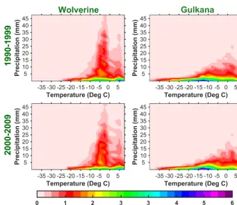
As expected from their respective geographies, the cli-mates of Gulkana and Wolverine watersheds are markedly different (Figs. 2 and A1). The hottest air temperatures (i.e., summer temperatures) are similar between Gulkana and Wolverine but Gulkana is significantly colder at the low end of the distribution (i.e., corresponding to colder winter tem-peratures at Gulkana). At all percentiles in the distribution, Wolverine’s precipitation is greater than Gulkana’s. Based on Gulkana being relatively drier and colder and Wolverine be-ing wetter and warmer, the watersheds can be classified, re-spectively, as continental and maritime (Armstrong and Arm-strong, 1987; O’Neel et al., 2014). These climate classifica-tions are consistent with findings for the Alaska region pre-sented in Bieniek et al. (2012) (using cluster analysis of sta-tion records) and Simpson et al. (2002) (based on Parameter-elevation Regressions on Independent Slopes Model interpo-lated climate surfaces; Daly et al., 2002).

Snowpacks in continental climates tend to be much more polythermal and less dense than snowpacks in maritime climates (Armstrong and Armstrong, 1987; DeWalle and Rango, 2008; Barry, 2008). Higher densities in maritime snowpacks are partially caused by atmospheric conditions

Figure 2.Cumulative probability distributions of daily precipita-tion and mean surface air temperature for the Gulkana and Wolver-ine watersheds (Fig. 1) from 1980 to 2009. The lWolver-ines correspond to the spatially averaged precipitation and temperature values and the shaded region indicates 1 standard deviation in the spatial distribu-tion of precipitadistribu-tion and temperature within the watershed. Climate representation is derived from the daily downscaled Climate Sys-tem Forecast Reanalysis (Saha et al., 2010) product discussed in Sect. 3.1.

during snowfall and also by repeat freezing and melting cy-cles, which are more common to under maritime conditions. These climatic differences in turn affect the thermal proper-ties of snow and ice because the thermal conductivity of snow is primarily a function of density and water content, and the snowpack properties impact the surface heat flux of glaciers when and where they are snow covered (Sturm et al., 1997; DeWalle and Rango, 2008).

glaciers’ respective classifications as maritime and continen-tal.

2 The Conceptual Cryosphere Hydrology Framework (CCHF)

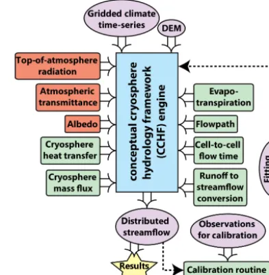
CCHF version 1 models alpine and glacier systems using nine process modules (see Fig. 3, Mosier, 2016). While it is common for conceptual cryosphere models to combine heat and snow/ice melt into a single formulation (e.g., Eqs. 1–3), CCHF represents these processes using two distinct modules, namely “cryosphere heat transfer” (referred to as the heat module for brevity; described in Sect. 2.1) and “cryosphere mass flux” (referred to as the mass flux module; described in Sect. 2.2). While we have programmed multiple representa-tions for each process module in CCHF, we only vary the heat module and mass flux module in this work. We choose this focus because the processes represented in these modules are the most sensitive to climatic differences (resulting from ei-ther interregional variability or long-term climatic changes). Section 2 describes the capabilities of CCHF and Sect. 3 out-lines the specific methods used to implement CCHF for the present model evaluation.

CCHF is designed to be easy to apply and extend. Presently CCHF can be applied to hourly, daily, or monthly time steps and any spatial grid expressed in uniformly spaced geographic coordinates. We have built in capability for CCHF to read precipitation, mean temperature, minimum temperature, and maximum temperature climate inputs. It would be straightforward, though, to expand CCHF for use with additional climate inputs. CCHF does not include meth-ods for correcting any of the climate inputs – any corrections must be undertaken during pre-processing of the climate in-puts. All heat flux terms, either conceptual (e.g., degree day factors) or physical (e.g., shortwave radiation), are parame-terized within CCHF.

The process representations for the seven fixed modules, provided in Table 2, are used because preliminary analysis indicated these representations work well for the conditions under which the CCHF is currently implemented. Section 2.4 discusses the modules involved in translating snow and ice melt and rain into streamflow, which are represented by the four modules on the right-hand side of the engine in Fig. 3. In addition to the nine process modules, CCHF also includes a built-in calibration routine (Fig. 3), which we discuss in Sect. 2.5.

We model the ratio of precipitation that falls as snow, rp

(also referred to as precipitation partitioning), using a linear ramp formulation

rp=   

 

1 ifTa≤Tp,s

Tp,r−Ta

Tp,r−Tp,s ifTp,s≤Ta≤Tp,r

0 ifTp,r≤Ta

, (7)

Figure 3.Categories of process modules included in version 1 of the Conceptual Cryosphere Hydrology Framework (CCHF). Rounded blocks refer to process modules and ovals refer to data inputs and outputs. Blocks tinted green denote modules used for all models and blocks tinted orange denote modules only used for models that include shortwave radiation.

whereTp,sis the threshold air temperature at which all

pre-cipitation falls as snow ([Tp,s]=◦C) andTp,r is the

thresh-old air temperature at which all precipitation falls as rain ([Tp,r]=◦C). The threshold temperatures at which all

pre-cipitation falls as snow and rain can be optimized or set. Throughout this work we set Tp,s=0◦C and Tp,r=2◦C.

We choose these threshold air temperatures because Beamer et al. (2016) optimizes this precipitation partitioning function (Eq. 7) for the Gulf of Alaska and finds that these temperature thresholds perform better than other sets of threshold temper-atures tested. Of note, Beamer et al. (2016) also find that the performance of SnowModel (the model they implement; Lis-ton and Elder, 2006a) is insensitive to modest perturbations in the precipitation partitioning parameters. A likely reason that the model is insensitive to these parameters for this re-gion is that Alaska has strong seasonal variations in temper-ature and winter tempertemper-atures are typically much colder than the mixed-phase precipitation zone. Therefore, we do not ex-pect the precise values to significantly impact results of our study and by setting the values fixed we reduce the dimen-sionality of our model calibration.

Table 2. Process representations for modules that are fixed in the present CCHF implementation.catm1andcatm2are fitting parameters

(unitless),1T is maximum temperature minus minimum temperature ([1T]=K), andP

Tmaxis the cumulative sum of maximum daily

temperatures since the last precipitation event ([P

Tmax]=K). Albedo of exposed ice is assumed to be 0.35.

Module name Representation Source

Top-of-atmosphere function of latitude, slope, aspect, and DeWalle and Rango (2008) radiation day of year

Atmospheric catm1

1−exp−0.01catm21T2.4

DeWalle and Rango (2008) transmittance

Albedo (snow) 0.90−0.55 log P

Tmax Pellicciotti et al. (2005)

Potential Eq. (22) Allen et al. (1998), evapotranspiration Lu et al. (2005) Flow path Sect. 2.4 manually determined Cell-to-cell flow Eq. (23) Johnstone and Cross (1949) time

Runoff to streamflow Sect. 2.4 Moore et al. (2012) conversion

2.1 Cryosphere heat transfer

Implementing the existing conceptual cryosphere models de-scribed by Eqs. (1)–(3) requires transforming their units be-cause all heat terms in CCHF have units of Watts per meter squared. We therefore define heat representations to use in CCHF that are analogs to these previous conceptual repre-sentations (i.e., Eqs. (1)–(3), respectively):

HSDI=cfm(Ta−T0) , (8)

HETI(H)= choc,s/iI+cfm(Ta−T0) , (9) HETI(P)=cpel(1−α)I+cfm(Ta−T0) , (10)

where the H terms are the net heat fluxes ([H]=W m−2; subscript “SDI” refers to the generic SDI model, “ETI(H)” refers to the ETI model described in Hock, 1999, and “ETI(P)” refers to the ETI model described in Pellicciotti et al., 2005), cfm is the degree-index factor

([cfm]=W m−2◦C−1), choc,s/i represents two fitting

pa-rameters, choc,sandchoc,i, which scale incoming shortwave

radiation, I, incident upon snow and ice, respectively ([ah,s/i]=◦C−1), and cpel is a fitting parameter to scale

the magnitude of shortwave radiation in the HETI(P)

representation (unitless).

We also implement and assess a novel conceptual heat rep-resentation, which we refer to as the longwave, shortwave, and temperature (LST) formulation. The LST representation is similar to ETI(P) except that LST includes a longwave ra-diation balance term and LST does not have a fitting param-eter to scale shortwave radiation. The LST heat flux,HLST

([HLST]=W m−2), is HLST=(1−α)I+cfmTa+σ

εa(Ta+273.15)4

−Ts,s+273.154

, (11)

where σ is the Stefan–Boltzmann constant (σ=5.67× 10−8W m−2K−4), εa is the effective atmospheric

emis-sivity (unitless), and Ts,s is the snow surface temperature

([Ts,s]=◦C). The LST formulation assumes εa to be 0.7

when there is no precipitation and 1 otherwise, which roughly translates to clear-sky and cloudy conditions (Hock, 2005; Sedlar and Hock, 2009). Unlike the SDI, ETI(H), and ETI(P) heat transfer representations (Eqs. 8–10), the LST representation requires modeling the snowpack and ice sur-face temperatures, which is discussed in Sect. 2.2.

2.2 Cryosphere mass flux

We implement two process representations within the mass flux module to relate the net heat flux to changes in the in-ternal energy and mass of snow and ice. The first representa-tion is a step funcrepresenta-tion, denoted asθ, which is implicit in the SDI and ETI formulations used in existing conceptual mod-els (i.e., Eqs. 1–3). The second mass flux representation is based on the cold content (Eq. 6) and is denoted as CC. In both theθ and CC mass flux representations, heat is trans-lated into melt potential,MP([MP]=m), which is analogous

toMin Eq. (5), through the relationship MP=

H 1t ρwLf

. (12)

greater than a threshold value, which is described mathemat-ically as

Mθ=

(

MP ifTa> cthr

0 otherwise , (13)

where cthr is taken to be a fitting parameter ([cthr]=◦C).

Therefore, combining the respective heat flux representations HSDI,HETI(H), andHETI(P)with theθ mass flux

representa-tion essentially allows us to reproduce the previous concep-tual models presented in Eqs. (1)–(3), albeit with different units for many of the fitting parameters.

Cold content in CC mass flux representation is denoted as wc([wc]=m) to distinguish it from the general definition of

CC in Eq. (6).wcis calculated as

wc,i=

(

wc,i−1−cccMP,i ifMP,i<0 wc,i−1−MP,i otherwise

, (14)

where subscript i refers to the current time step, subscript “i−1” refers to the previous time step,ccc is a unitless

fit-ting parameter that provides a hysteresis in the accumulation and depletion ofwc, andMPcan be either positive or

nega-tive (determined by sign ofHin Eq. 12). The lower bound on wc is zero (i.e.,wcis set to zero if it becomes negative) and wcis always zero at grid locations without snowpack,

includ-ing those with ice but no snow. Physically, the CC hysteresis relates to differences in the conduction of energy through the snowpack during accumulation (dry) versus ablation (wet) conditions. Melt in the CC mass flux representation, MCC

([MCC]=m), is calculated as

MCC= (

MP−wc ifMP> wc

0 otherwise . (15)

While snowpack temperature cannot be modeled in theθ representation, the CC representation models the average in-ternal snowpack temperature,Ts,i, as

Ts,i= −ctsnwc, (16)

where ctsn is a fitting parameter to translate wc into

inter-nal temperature ([ctsn]=◦C m−1). Thus, the assumption is

made in the CC representation that the snowpack is isother-mal (i.e.,Ts,i=Ts,s). When liquid water in the snowpack is

greater than 0.5 % of solid snow water equivalent (SWE), the snowpack temperature is set to 0◦_{C. The LST heat} repre-sentation is the only formulation implemented here that uses Eq. (16) and in this case it is assumed that the snow surface temperature,Ts,sin Eq. (11), is equal to the snowpack’s

aver-age internal temperature,Ts,iin Eq. (16). This is equivalent

to a strict isothermal snowpack assumption, which is more realistic for wet and warm snowpacks than for dry and cold snowpacks. Based on the climates of Gulkana and Wolverine (Figs. 2 and A1), we expect this to be a better assumption for Wolverine than Gulkana.

Both the θ and CC mass flux representations con-tain a maximum snowpack liquid water content, MLC ([MLC]=m), represented by

MLC=cslqSWEs, (17)

wherecslq is a unitless fitting parameter and SWEs is the

snowpack’s solid water content expressed as depth of liq-uid water equivalent ([SWEs]=m). All liquid water in

ex-cess of the snow’s liquid water holding capacity drains from the snowpack during each time step. In the CC formulation, the snowpack’s liquid water is refrozen when CC is greater than 0, and the CC is reduced in direct proportion to the depth of water frozen. Only water that drains from the snowpack is counted as a change in the snowpack’s total water content. 2.3 Glacier treatment

Fully representing ice processes requires accounting for the ice’s internal energy. Conceptual models typically do not do this, instead assuming the ice temperature is 0◦C when there is no snow present and the heat flux into the ice is positive (Hock, 1998, 1999). The present version of CCHF does not include any mass flux modules that account for the inter-nal energy of ice, although this is an area that we believe should be developed in the future. Instead, CCHF assumes the glacier surface albedo is 0.35 and that the glacier’s sur-face temperature is the minimum of the air temperature in the previous time step and 0◦C. The glacier’s surface tem-perature only impacts net longwave heat flux calculated in the LST model.

During a given time step, ice melt potential, MP,ice

([MP,ice]=m), is calculated as the remainder of potential

melt after snow melt is calculated, i.e., MP,ice=

(

MP−M ifMP> M

0 otherwise . (18)

Actual ice melt, Mice ([Mice]=m), is scaled by a unitless

fitting parameter,cglc, that accounts for energy differences

in melting ice versus snow (e.g., accounting for differences in heat conduction between ice and snow). Thus, ice melt is calculated as

Mice=cglc Hice

H MP,ice, (19)

whereHiceis the heat flux for the ice surface properties and His the equivalent heat flux for snow surface properties. For a given model implementation, bothH andHicecorrespond

to the same heat flux representation (i.e., one representation from Eqs. 8–11). For example, for the model whereHETI(P)is

used as the heat representation, the only difference between H andHice in Eq. (19) is due to the difference in surface

approximates the portion of energy that is still available for ice melt after all snow has melted during the current time step. Over short time steps, the error incurred by not allow-ing snow and ice melt to occur for a given grid cell durallow-ing the same time step is small; however, including Eq. (19) allows the model to scale better between small and large time steps. 2.4 Melt and rain to streamflow

Once liquid water drains from the snowpack, ice melt occurs, or rain is incident on a grid cell without snow, CCHF els its transport through the landscape with the four mod-ules on the right side of Fig. 3. Two general phases of this transport are (1) transition from snow or ice melt to runoff and (2) flow through the stream network. To model phase one, we implement a leaky groundwater bucket model as de-scribed in Moore et al. (2012). In the bucket representation, all liquid water released from snow, snlr ([snlr]=m), liquid water released from ice, iclr ([iclr]=m), and rain incident on a grid cell without snow ([rain]=m) enters the ground-water bucket. The ground-water in the bucket is described as the soil moisture, SM ([SM]=m), with a total soil moisture capacity, csmc([csmc]=m;csmcis a fitting parameter). SM is updated

during each time step as

SMi=

SMi−1+raini+snlri+iclri−rf,i−PETi if no snow or ice present

SMi−1+raini+snlri+iclri−rf,i otherwise

, (20) where subscript i refers to the value during the ith time step and PET is potential evapotranspiration ([PET]=m; de-scribed below). Runoff, rf ([rf]=m3day−1), in the bucket

model is then calculated based on SM andcsmcas

rf= (

A ((1+cdr)SM−csmc) if SM≥csmc

AcdrSM otherwise

, (21)

whereAis the grid cell’s area ([A]=m2) andcdris the drain

rate of soil moisture from the leaky groundwater bucket per day ([cdr]=day−1; fitting parameter ranging from 0 to 1).

PET is calculated using a formulation of the Hamon equa-tion (Hamon, 1961) based on Allen et al. (1998) and Lu et al. (2005), in which

PET=218.39×cpet×N 



6.108 exph 17.27Ta

Ta+273.15 i

Ta+273.15 

, (22)

wherecpetis a unitless fitting parameter andNis the number

of daylight hours ([N]=h), which is calculated according to the formulation presented in DeWalle and Rango (2008). PET is set to zero when snow or ice is present.

Flow direction between grid cells in CCHF can be input by the user (in the form of an Environmental Systems Research Institute – ESRI – formatted flow direction grid) or calcu-lated automatically using algorithms from the TopoToolbox

(Schwanghart and Kuhn, 2010). The travel time through each cell, tt ([tt]=s), is then calculated using a formulation by

Johnstone and Cross (1949):

tt=3600ctvl s

1l √

m, (23)

wherectvlis a unitless fitting parameter,1lis the distance

be-tween the centroids of grid cells in the flow path ([1l]=m), andmis the slope between cells in the flow path expressed as a ratio (unitless).

Streamflow is then routed downhill along the flow path de-termined by the flow direction grid using either the “lumped” or Muskingum methods (Bedient et al., 2012). The lumped method does not allow dispersion of streamflow, whereas the Muskingum method does allow dispersion according to the formulation presented in Bedient et al. (2012). The results of both flow routing methods are comparable for simulating small watersheds at large time steps; however, dispersion be-comes more important as the size of the watershed increases relative to the time step (Bedient et al., 2012). In this work we use the lumped method since the model domains are small. 2.5 Calibration routine

Several calibration routine options are built into the CCHF, including a genetic algorithm (Wang, 1991), Monte Carlo simulation (Sawilowsky and Fahoome, 2003), Particle Swarm Optimization (PSO; Poli et al., 2007), and a hybrid al-gorithm developed by us. The hybrid alal-gorithm works by im-plementing the Monte Carlo routine for the first several cali-bration generations (ranging from 4 to 15 generations based on the number of fitting parameters) and updating the fitting parameters in the following generations using PSO until two consecutive generations stagnate to the same fitness score (referred to here as an initial stagnation). Once an initial stag-nation occurs, the hybrid algorithm uses a combistag-nation of Monte Carlo simulations and linear sensitivity analysis to al-ternately add diversity to the population (Monte Carlo simu-lation) and explore the local parameter space (linear sensitiv-ity). If a new local optima is found, PSO is reinitiated. The process repeats until the same best fitness score is returned for 15 consecutive generations (referred to here as terminal stagnation). A population of 30 parameter sets is used in each generation of the optimization process.

and Blöschl, 2008). The NSE and KGE scores are computed for glacier stake and streamflow comparisons while the PBE score is computed to compare SCA observations to modeled snow as described below.

The NSE score is extensively used to assess hydrologic models and, as is shown in Gupta et al. (2009), can be de-composed into the form

NSE=2αr−α2−β2, (24)

whereαis the ratio of the model standard deviation to the observed standard deviation,r is the linear correlation coef-ficient, andβis the bias normalized by the observed standard deviation. From Eq. (24) it is evident that the NSE score un-equally weights standard deviation, correlation coefficient, and bias. Therefore, Gupta et al. (2009) propose using the KGE score, defined as

KGE=1−

q

(r−1)2_+(α−1)2_+(β−1)2_{, (25)}

which equally weights errors in the correlation, standard de-viation, and the non-dimensional bias.

A perfect KGE or NSE score is 1 and the negative bound on the scores is negative infinity. An NSE score of 0 indicates the mean of the observation time series is as good of a pre-dictor as the modeled time series. Note, though, that a KGE score of 0 does not share this interpretation. The advantage of using the KGE for calibration instead of the NSE is that the NSE is sensitive to errors in extreme values and less sen-sitive to errors in the overall distribution relative to the KGE metric (Legates and McCabe Jr., 1999).

Using MODIS SCA observations for model evaluation presents a unique challenge since MODIS observes snow and ice cover while CCHF models SWE. The PBE score over-comes this issue by calculating two error metrics – snow overestimation error, S_EO (unitless), and snow underestima-tion error, S_EU (unitless) – which, respectively, capture in-stances where the model grid cell contains snow but the MODIS pixel does not report SCA and instances where the model grid cell does not contain snow but the MODIS pixel reports SWE.S_EOandS_EUare calculated as

S_EO= 1 ml

l

X

j=1

mo∧(SWE> ξSWE)∧(SCA=0), (26)

S_EU= 1 ml

l

X

j=1

mu∧(SWE=0)∧(SCA> ξSCA) , (27)

wheremis the number of number of MODIS time steps in which less than 60 % of the MODIS image over the entire domain is cloud covered (images with cloud cover greater than this threshold are not used),lis the number of grid cells that are not glaciated or have permanent snow cover (these MODIS pixels are also removed from analysis as explained below), the summation overj loops over all MODIS pixels

that contribute tol,mois the number of MODIS time steps

for which MODIS reports 0 % snow cover at the current grid cell and modeled SWE is greater than a threshold value set byξSWE([ξSWE]=m), andmuis the number of MODIS time

steps where no SWE is modeled at the current grid cell but MODIS observes snow cover greater than ξSCA (unitless).

Due to potential issues in which MODIS incorrectly classi-fies permanent ice as snow, we remove all MODIS pixels from analysis when a given pixel is classified as snow dur-ing more than 90 % of the time steps. Thus, MODIS data are only used in model evaluation for grid cells with seasonal snow cover and not for grid cells that MODIS classifies as having permanent snow.

The PBE score is calculated fromS_EO andS_EU using the weighting function

PBE=w1SEO+w2SEU, (28)

where PBE is the snow cover error used in model assess-ment (unitless; range is 0 to 1, where 0 indicates no error) andw1 andw2 are unitless weighting factors used to scale

the model overestimation and underestimation errors, respec-tively.

S_EO and S_EU, respectively, decrease as ξSWE and ξSCA

increase. Thus, errors are largest with ξSWE=0 m and ξSCA=0 %. Parajka and Blöschl (2008) set the values of ξSWEandξSCAin order to balanceSEOandSEU. Unfortunately

it is not possible to balanceS_EOandS_EUa priori in the present implementations because the sensitivity ofS_EOandS_EU with respect toξSWEandξSCAchanges between model domains,

model formulations, and with different fitting parameter val-ues. We setξSWE to 10 mm and ξSCA to 10 % in order to

increase the sensitivity of the calibration to bothS_EOandSU_E. We do not set theξ values to 0 in order to recognize that there can be classification errors in MODIS SCA observations for pixels with low snow cover and because CCHF assumes all snow is uniformly distributed over the grid cell, whereas at very low SWE values this is not likely to be accurate. We setw1andw2in Eq. (28) to 5 because we find through

ini-tial calibration analysis that this tends to result in PBE having similar magnitudes to KGE values computed for glacier stake observations.

3 Methods for model comparison

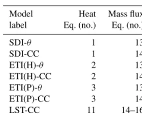
Table 3.Heat module and mass flux module combinations that we assess, described, respectively, in Sects. 2.1 and 2.2. In all cases the seven fixed module formulations are those presented in Table 2.

Model Heat Mass flux label Eq. (no.) Eq. (no.) SDI-θ 1 13 SDI-CC 1 14 ETI(H)-θ 2 13 ETI(H)-CC 2 14 ETI(P)-θ 3 13 ETI(P)-CC 3 14 LST-CC 11 14–16

calibrating the models in two stages, and conducting cali-bration for 10 consecutive water years in which all obser-vation data are available. Reducing equifinality helps enable intercomparison of model accuracy and precision. We addi-tionally assess how much equifinality is present in each of the seven calibrated models. Section 3.1 describes the in-puts used in these implementations of the model, Sect. 3.2 then provides information on the observation data used, and Sect. 3.3 explains the evaluation strategy.

3.1 Model inputs

CCHF presently supports inputs of precipitation and temper-ature (mean, minimum, and maximum) time series, a digi-tal elevation model (DEM; we use the WorldClim 30 arcsec DEM by Hijmans, 2011), a data file containing outlines of glacier or ice cover, and a flow direction raster (FDR). The FDR can be generated automatically within CCHF using al-gorithms from the TopoToolbox, Schwanghart and Kuhn, 2010; however, we manually delineate the watersheds and create the FDR using a combination of ESRI algorithms and visual analysis.

The climate time series inputs used here are derived from the Climate Forecast System Reanalysis (CFSR), which is produced by the National Centers for Environmental Predic-tion (NCEP) (Saha et al., 2010). CFSR is an hourly climate product available from 1979 to 2010 as 0.312◦grids. Wang et al. (2011) and Lader (2014) find that CFSR represents pre-cipitation and temperature variability as well or better than other reanalysis products such as MERRA (Rienecker et al., 2011) and ERA-Interim (Dee et al., 2011) for the Alaska re-gion. Further, Beamer et al. (2016) find that CFSR performs well relative to other reanalysis products for Gulkana and Wolverine glaciers and also better reproduces total volumes of water flux into the Gulf of Alaska.

We temporally aggregate the hourly 0.312◦CFSR product to daily time steps. Precipitation and mean temperature are used in all instances, while minimum and maximum temper-ature are only used in model formulations that include short-wave radiation. We input the temporally aggregated 0.312◦

CFSR product into MicroMet (Liston and Elder, 2006b). Mi-croMet resamples the input time series to the spatial grid of the DEM and applies temperature lapse rates and precipita-tion correcprecipita-tion factors based on elevaprecipita-tion distribuprecipita-tion, which vary as a function of the day of the year, creating a 30 arcsec daily time series for each climate variable.

Glacier outlines in CCHF can be supplied in gridded for-mat using the same grid as the input DEM or can be input as a shapefile. In the case where a shapefile is input to the model, CCHF determines the fractional area of glacier cov-erage within each of the model’s grid cells. We use the Ran-dolph Glacier Inventory version 5 shape files (Pfeffer et al., 2014) to generate the glacier outlines in this work and hold these outlines fixed over the duration of each model run. 3.2 Observation data

The three types of observation data we use to assess model performance are USGS stream gage measurements of flow rate (referred to in the results as “flow”), MODIS (Hall et al., 2006) images of SCA (referred to as “SCA”), and USGS glacier stake measurements of changes in snow and ice water equivalent (referred to as “stake”). Gulkana and Wolverine are both considered long-term benchmark glaciers by the USGS, with the implication that glacier stakes and stream gages have been present at both locations for multiple decades, albeit with some interruptions as described below.

The USGS has been measuring glacier and snow accu-mulation and ablation at three locations on Gulkana glacier from 1974 through the present (with an additional stake from 1990 through the present) and three locations on Wolverine from 1965 through the present (Van Beusekom et al., 2010). Glacier stakes measure changes in depth of snow and ice at one location between two observation dates. These changes in depth are then converted to changes in mass through measuring the density of snow and assuming a den-sity for ice. Wolverine glacier is entirely free of surface de-bris, while a portion of the ablation zone of Gulkana glacier contains scattered debris cover, but we model both glaciers as debris free. In our analysis, we treat each glacier stake obser-vation equally, regardless of duration, season, or magnitude of change.

There are stream gages located slightly below the termini of Gulkana and Wolverine glaciers. The stream gages were installed in 1966 and are maintained by the USGS. The tem-poral coverage of the stream gages is not continuous. For ex-ample, the stream gage at Gulkana is missing measurements from October 1978 through September 1989 and the stream gage at Wolverine does not have measurements from Octo-ber 1978 through SeptemOcto-ber 2000. The USGS also cautions that there may be significant errors in the flows, especially at high flows, because the stream gages are located in geomor-phologically active channels.

using a Sinusoidal tile grid, available from March 2000 through the present (Hall et al., 2006). We use the 8-day im-ages rather than daily because cloud cover obstructions are a significant hindrance in the daily product and Zhou et al. (2005) achieve better performance using the 8-day time se-ries rather than the daily. MOD10A2 version 5 provides a bi-nary classification for each pixel (i.e., either snow, no snow, or no decision). When 60 % or more of the pixels in a current image corresponding to one of the study domains is no de-cision, we set the entire image to no decision (this threshold is also used in Parajka and Blöschl, 2008). We then reproject the image to geographic coordinates and resample the images to our model domains using bilinear interpolation. Therefore, the SCA values used in model assessment can range from 0 to 100 %.

3.3 Evaluation strategy

Our primary goal with the model intercomparison is under-standing how each of the seven models in Table 3 performs under different climatic regimes (as a partial analog for cli-mate change applications) and across geographies (because models are often calibrated for gaged watersheds but ap-plied to non-gaged watersheds). Due to this, we calibrate each model to both Gulkana and Wolverine domains sepa-rately and then validate each model for the opposite water-shed (i.e., we perform a total of 14 model calibrations and 14 model validations). We spin up each of the model runs from September 1997 through August 2000 and then con-duct each calibration or validation assessment from Septem-ber 2000 through August 2010.

The combined use of MODIS, glacier stake, and stream gage observations has been shown to significantly improve model performance and better differentiate performance of model parameter set ensemble members (Konz and Seibert, 2010; Finger et al., 2011). By only evaluating models for the period 2000–2010, we are able to use all three observation types and therefore utilize a stronger evaluation criteria for each model. We view the 10-year calibration and validation periods as necessary to assess performance over a range of climatic conditions and reduce equifinality. Often models are assessed for shorter periods (e.g., Singh et al., 2000; Liston and Mernild, 2012; Hock and Holmgren, 2005) but there is evidence that assessing models over short periods can lead to incorrect assessments (e.g., see Razavi and Tolson, 2013).

We calibrate each model in two stages. In the first stage, parameters relating to cryosphere modules (see Fig. 3) are optimized by maximizing the average of 1 minus the PBE score for MODIS SCA relative to modeled SWE and the KGE value between measured and modeled changes in SWE and ice water equivalent at glacier stake changes (see details in Sect. 2.5). In the second stage, the calibrated cryosphere parameters are then set to their optimized values and all re-maining parameters (i.e., those related to runoff generation and routing processes; see Sect. 2.4) are optimized by

maxi-Figure 4. Model flow performance during calibration and vali-dation as a function of combined cryosphere performance using the methodology and metrics described in Sects. 2.5 and 3.3. In subplot(a), models are calibrated for Gulkana and validated for Wolverine; in subplot(b), models are calibrated for Wolverine and validated for Gulkana. As indicated in the plot legends, the marker border indicates phase of assessment, face color indicates the heat module representation, and shape indicates the mass flux module representation.

mizing the KGE score for modeled and measured streamflow at the USGS stream gage locations. Since glacier stake ob-servations are available at multiple points, fitness scores dur-ing the first stage of calibration are calculated at each glacier stake location and then averaged to produce a single glacier stake score for each parameter set.

We assess equifinality due to the cryosphere process rep-resentations by conducting validation on the 100 parameter sets that perform best during the first stage of calibration. We set the fitting parameters corresponding to non-cryosphere parameters (i.e., those calibrated in the second stage) to their calibrated values. Thus, we are only investigating equifinal-ity in fitting parameters related to modeling cryosphere pro-cesses. We provide equifinality assessment statistics in all ta-bles of validation run results. Specifically, we include (1) val-idation performance for the parameter set that performs best during calibration, (2) the mean validation performance for the 100 best performing calibration runs, and (3) the standard deviation of validation performance for the 100 best perform-ing calibration runs. The general format we use for reportperform-ing these statistics is “x1;x2±x3”, where thexirefer to the three numbered statistics from the previous sentence.

4 Results and discussion

cor-responding calibrated fitting parameter values are provided in Tables B1 and B2. While Fig. 4 efficiently summarizes the results, trends become more apparent when model per-formance is aggregated in specific ways. We therefore sep-arate this section into several subsections to highlight inter-esting aspects of the model intercomparison results. Some of the findings are as follows: (1) which mass flux mod-ule representation performs best depends on the watershed (Sect. 4.1); (2) overall performance varies between the two watersheds (Sect. 4.2); and (3) which model formulations performs best depends on the observation variable consid-ered, but the ETI(P)-CC and LST-CC models stand out as the most accurate and robust between regions (Sect. 4.3). Sec-tion 4.5 then summarizes general observaSec-tions.

We also want to note at the outset that the choice of metric, as well as the overall assessment methodology, are significant determinants of perceived model performance. We primarily use and report the KGE score (Eq. 25) for glacier stake and flow observations and the PBE score (Eq. 28) for SCA obser-vations, although Tables B3–B5 provide model performance quantified by the NSE score (Eq. 24) as well. As is displayed in Sect. 2.5, the KGE and NSE scores can be decomposed into three principal sources of error (i.e., correlation, standard deviation, and bias). As is outlined in Gupta et al. (2009), the relative importance of each of the three additive terms in Eqs. (24) and (25),Fi, can be calculated as

Fi= fi

3 P

j=1 fj

, (29)

wherefi are values of the respective terms. To demonstrate how each error component impacts the overall KGE and NSE scores, Table 4 provides the stake error components corre-sponding to validation runs for the LST-CC model. What is important to note is that the first term of the NSE score (2αr/P_[

ni]) is negative for both watersheds and therefore masks some of the error in the other two terms, which relate to the standard deviation and bias. This potential for error masking in the NSE score explains one factor contributing to higher NSE scores relative to the corresponding KGE scores (see Tables B3–B5).

Another finding from Table 4 is that the largest sources of KGE error for Gulkana are the correlation coefficient and standard deviation components, while the largest sources of error for Wolverine are the correlation coefficient and bias components. The cause of these respective errors cannot be ascertained from Table 4 without more investigation; how-ever, this type of information may be informative for improv-ing the future model representations.

Many other modeling studies implement similar concep-tual models and report “better” model performance. “Better” is placed in quotation marks because, as is shown in Table 4, what constitutes better depends on the metric used and how the model is assessed. Commonly glacier models are

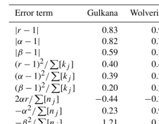
eval-Table 4.Sources of stake measurements errors in the Kling–Gupta efficiency (Eq. 25) score in the LST-CC model during validation for Gulkana and Wolverine glaciers. The three error types are the linear correlation coefficient,r, the ratio of the model standard deviation to the observed standard deviation,α, and the bias normalized by the observed standard deviation,β.P

[kj]andP[nj]refer to the sum

of additive terms for the KGE score and NSE score, respectively (i.e., the denominator on the right-hand side of Eq. (29).

Error term Gulkana Wolverine

|r−1| 0.83 0.96

|α−1| 0.82 0.73

|β−1| 0.59 0.83

(r−1)2/P_[

kj] 0.40 0.43

(α−1)2/P

[kj] 0.39 0.25

(β−1)2/P_[

kj] 0.20 0.32

2αr/P

[nj] −0.44 −0.27 −α2/P_[

nj] 0.23 0.91 −β2/P

[nj] 1.21 0.36

uated for only a few years (e.g., Liston and Mernild, 2012) or only during the melt season (e.g., Singh et al., 2000; Pel-licciotti et al., 2005). Additionally, models evaluated using fewer types of observations tend to appear to perform bet-ter (Konz et al., 2010; Finger et al., 2015). It has also been demonstrated by Razavi and Tolson (2013) that when cali-brating and validating hydrologic models, use of short du-rations can lead to inaccurate assessments of model perfor-mance and increase model equifinality. In the context of iden-tifying robust models for use in projecting the impacts of cli-mate change, it is therefore necessary to ensure that the val-idation utilizes a sufficient number of types of observation data, that the evaluation period is sufficiently long, and that evaluation is conducted for multiple climatic regimes. 4.1 Mass flux module

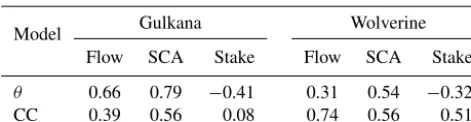
Average performance of the two mass flux representations, θ and CC, tends to vary by watershed (Table 5). On aver-age theθrepresentation performs better for Gulkana and the CC representation performs better for Wolverine. A differ-ence between these watersheds is that Gulkana is drier and colder than Wolverine (Figs. 2 and A1). Although it is be-yond the scope of the present work to establish precisely why theθrepresentation performs better for Gulkana and the CC representation performs better for Wolverine, it may be re-lated to the way each module represents the timing of accu-mulation and melt.

Table 5.Evaluation scores during model validation by mass flux module representation and watershed, averaged over heat module representation. The watershed listed is that which the model is val-idated for. Evaluation methodology and metrics are described in Sects. 2.5 and 3.3.

Model Gulkana Wolverine Flow SCA Stake Flow SCA Stake

θ 0.66 0.79 −0.41 0.31 0.54 −0.32 CC 0.39 0.56 0.08 0.74 0.56 0.51

for less dense snowpacks, which causes energy changes at the surface to propagate more slowly through the low-density snowpack relative to a higher-density equivalent snowpack. By this mechanism, the CC representation may overestimate internal energy deficit during dry and cold winter months, which would impact models applied to Gulkana more than models applied to Wolverine.

One characteristic of an improved mass flux representa-tion would be that it allows snowpack temperature to vary vertically through the snowpack. This would have two ad-vantages over the CC representation: (1) the net surface heat fluxes could be better calculated across climatic regimes and (2) the effect of the snowpack’s thermal conductivity could be accounted for in updating the snowpack’s average inter-nal energy. An approach to accomplish this would be to it-eratively solve for the surface temperature by requiring that the surface energy balance be zero, as is done in Liston and Elder (2006a). Using such a method, melt would occur based on the energy balance at the surface of the snowpack rather than as a function of the snowpack’s average internal energy, as is the case in the CC representation.

4.2 Regional differences

If validation results are aggregated over model applications to the same region, it appears that on average the seven mod-els better reproduce stake observations for Wolverine and better reproduce SCA observations for Gulkana. Simulta-neously, though, they reproduce flow observations roughly equally well (Table 6). One important caveat is that averaging over models ignores intermodel differences in performance. To better understand causes of interregional model perfor-mance, we also calculate the linear correlation coefficient,r, between performance in each of the cryosphere observation types (i.e., SCA and stake) and flow, by region (Table 6). For Wolverine, the correlation between stake and flow perfor-mance is 0.99, while for Gulkana the correlation is not statis-tically significant. For Gulkana, the correlation between SCA and flow performance is 0.86, while for Wolverine the corre-lation is not statistically significant. One reason why stake performance may be more important to Wolverine is that a larger portion of the model domain and area contributing to

Table 6.Model-averaged evaluation performance scores and linear correlation coefficient,r, between performance of each cryosphere observation type and flow during model validation, shown by re-gion. The watershed listed is that which the model is validated for. The top row for each watershed is the regionally averaged evalua-tion score; the first number in parentheses isrand the second num-ber is thepvalue, which is an indicator of statistical significance (typically values less than 0.05 are considered significant). Evalua-tion methodology and metrics are described in Sects. 2.5 and 3.3.

Region Flow SCA Stake Gulkana 0.51 0.65 −0.13

(0.86; 0.012) (0.43; 0.33) Wolverine 0.56 0.55 0.15

(0.20; 0.66) (0.99; 0.00)

the stream gage is glacier covered. It is surprising, though, that for Wolverine SCA performance is not significantly cor-related to flow performance. We are not sure why SCA and flow performance are not correlated for Wolverine.

4.3 Model accuracy, precision, and equifinality

The primary model assessment goal of this work is to evalu-ate the robustness of the seven conceptual cryosphere models between regions and climatic conditions. Two aspects of ro-bustness are overall accuracy (i.e., predictive skill for each model application) and precision (i.e., how the predictive skill varies between applications of the model across regions and climatic conditions). Additionally, equifinality affects ro-bustness insofar as different equally acceptable parameter sets selected through calibration may lead to different inter-pretations of model results. Tables B4 and B5 display results of the equifinality exercise described in Sect. 3.3. In roughly half of the validation cases, the mean validation performance of the 100 best calibration parameter sets is slightly higher than the validation performance of the parameter set that per-forms best during calibration; the differences between these two metrics are almost always very small, though. Given that the assessment criteria includes flow, SCA, and stake ob-servations and that the validation assessment is particularly stringent (i.e., applying the calibrated models to a different model domain with a different climatic regime), we believe this level of equifinality is acceptable. For example, the dif-ferences in model performance are smaller than those ob-tained in Finger et al. (2011) and Razavi and Tolson (2013), although because of differences in each assessment approach it is not possible to make quantitative comparisons.

re-Table 7.Regionally averaged evaluation scores during model val-idation by model. Values in parentheses are absolute difference in model validation scores between regions. Evaluation methodology and metrics are described in Sects. 2.5 and 3.3.

Model Flow SCA Stake Mean SDI-θ 0.58 0.68 −0.04 0.41

(0.46) (0.19) (0.25) (0.30) SDI-CC 0.28 0.47 −0.20 0.18 (0.66) (0.26) (0.88) (0.60) ETI(H)-θ 0.48 0.69 −0.42 0.25

(0.26) (0.21) (0.29) (0.25) ETI(H)-CC 0.50 0.54 0.31 0.45 (0.48) (0.07) (0.34) (0.30) ETI(P)-θ 0.40 0.63 −0.65 0.13

(0.32) (0.34) (0.23) (0.30) ETI(P)-CC 0.75 0.60 0.51 0.62 (0.12) (0.07) (0.27) (0.15) LST-CC 0.73 0.62 0.56 0.64 (0.12) (0.12) (0.20) (0.15)

producing SCA observations. The precision, i.e., how simi-lar performance is between applications, for the ETI(P)-CC and LST-CC models is better than for the other five mod-els, including for SCA performance. While there are minor differences in performance between the ETI(P)-CC and LST-CC models (e.g., with respect to stake performance), the dif-ferences in performance between these two models are rela-tively small compared to differences with the other five mod-els. Therefore, we conclude that both the ETI(P)-CC and LST-CC models are superior to the other five models eval-uated in terms of validation accuracy and precision.

The novel conceptual model formulations that we assess include the four that utilize the CC mass flux representa-tion (i.e., the SDI-CC, ETI(H)-CC, ETI(P)-CC, and LST-CC models). If we compare only the pre-existing models (i.e., SDI-θ, ETI(H)-θ, and ETI(P)-θ), the SDI-θmodel ex-hibits the best flow performance, the SDI-θ and ETI(H)-θ models exhibit the best SCA performance, and the SDI-θ model exhibits the best stake performance (Table 7). On av-erage, the SDI-θ model outperforms the other models with θ mass flux representations, but none of these three pre-existing models is precise between watersheds. One signif-icant difference between these three models is that the SDI-θ model relies only on temperature both for determining the heat flux and onset of melt conditions, while the ETI(H)-θ and ETI(P)-θ models use both temperature and shortwave radiation to determine the heat flux but only temperature to determine onset of melt conditions. The latter set of process representations is not physically consistent given that in real-ity onset of melt conditions is determined by the energy bal-ance, which is impacted by all of the heat fluxes. This is not to claim that the SDI-θmodel is more physically

representa-Figure 5.Model performance for Gulkana using Gulkana calibra-tion (i.e., parameters from Table B1) and validating each model for Gulkana from September 1990 through August 2000. Only stake and flow observations are available during this validation period. The marker border indicates the whether the model period is cali-bration or validation, face color indicates heat module representa-tion, and shape indicates mass flux module representarepresenta-tion, as de-scribed in the legends.

tive than the others, just that the heat and melt formulations may be more consistent.

4.4 Assessment using Gulkana only

In this section we provide results for a model assessment us-ing only Gulkana watershed. The purpose of this is to under-stand the importance of the two-watershed model assessment methodology (described in Sect. 3.3), in which the water-sheds have contrasting climates and geographies, that we use to produce all of the model evaluation results provided else-where in this paper. For the Gulkana-only assessment, we use the model parameter sets displayed in Table B1, which are calibrated for Gulkana from September 2000 through August 2010. We then validate these calibrated models for Gulkana from September 1990 through August 2000, using the preceding 36 months as a model a spin-up period. Only stake and flow observations are available for this validation period. We cannot conduct a similar validation for Wolverine because stake observations are not available for this period.

highlights the importance of selecting an evaluation method-ology that tests model behavior over the range of conditions that the model will be applied for. As an example, if the ob-jective is to simulate recent historic conditions at Gulkana, the one-watershed assessment is appropriate and finds that the ETI(H)-θmodel should be used. If the model will be ap-plied to altered climatic or geographic conditions, the two-watershed assessment tests model performance over a wider range of conditions and finds that either the ETI(P)-CC or LST-CC models may be more suitable.

4.5 General remarks and future directions

As discussed in Fujita and Ageta (2000), glacier surface pro-cesses are not sufficient to describe glaciers; for example, because up to 20 % of melt refreezes. Surface refreezing is allowed in the CC mass flux module representation for snow-packs when the CC is positive, but not for glaciers. The pri-mary differences between snow and ice heat fluxes in the models implemented here are that (1) ice has a different sur-face albedo than snow and (2) ice includes a fitting param-eter to allow heat fluxes to translate into melt at a different rate than for snow (see Sect. 2.3). None of the models con-tains a representation of the ice’s internal energy. Even Snow-Model, an energy balance cryosphere hydrology model, does not characterize the internal energy of ice (Liston and Elder, 2006a). However, conceptual and energy balance cryosphere hydrology models are often applied to assess the impacts of glacier melt on projected future streamflow. We therefore perceive this as a significant deficiency in current cryosphere hydrology models and an area where future work must be done.

None of the cryosphere hydrology models implemented here uses wind speed or humidity as inputs, but these vari-ables are needed to explicitly represent the sensible and latent convective heat fluxes. The choice to exclude these inputs is made because they are less frequently observed for mountain environments, are difficult to characterize at high spatial res-olutions, and are therefore not commonly used in conceptual models. For continental snow and glacier environments, such as Gulkana, sublimation is an appreciable source of negative mass flux (Ohmura, 2001; DeWalle and Rango, 2008; Sicart et al., 2008). Similarly, sensible convection is important dur-ing the times of the year when the air and snow/ice surface temperatures differ from one another the most (e.g., late sum-mer during the glacier ablation season). Each of the concep-tual models we implement accounts for sensible heat fluxes through a degree-index term, which is a significant abstrac-tion from the actual process. In reality convective heat fluxes also depend on the wind speed and whether the atmosphere is in a stable, unstable, or neutral state (DeWalle and Rango, 2008). A potentially enlightening future experiment would be to develop a heat module representation that uses wind speed as an input and compare how uncertainties in charac-terizing wind speed impact representation of the heat balance

relative to using a degree-index term. The same experiment could be conducted for humidity to directly account for sub-limation.

5 Conclusions

Understanding how the cryosphere will respond to cli-matic changes has important water resources implications and requires implementing models that are robust across geographic domains and climatic conditions. Conceptual cryosphere hydrology models are often used to make these types of projections in mountain environments due to data paucity, yet existing conceptual models are known to be less robust than physically based model structures. We have de-veloped the CCHF (Fig. 3) in order to systematically assess cryosphere modeling assumptions. We use the CCHF here to implement seven conceptual models (including existing and novel formulations; Table 3) for two glaciated watersheds in Alaska (Fig. 1). The CCHF enables us to interchange individ-ual module representations, which provides more insight into the causes of differences in model performance compared to if we were to implement standalone models. While no sin-gle model outperforms the others for all categories of ob-servations, the ETI(P)-CC and LST-CC models stand out as overall the most accurate and precise between climatic con-ditions and geographic domains when model performance is assessed using flow, SCA, and stake observations.

Our model analysis is by no means exhaustive, but pro-vides some general insights and directions for future inves-tigations. For example, we find that theθmass flux module representation results in better model validation performance for Gulkana (the colder and drier of the two watersheds) and that the CC mass flux module representation results in better model validation performance under the same analy-sis for Wolverine (Table 5). Neither of these representations captures the impact of vertical temperature gradients within a snowpack on internal energy or on heat fluxes across the boundary. These deficiencies in cryosphere model formula-tions are consistent with other conceptual models (e.g., Hock, 1999; Pellicciotti et al., 2005) and even with energy balance models such as SnowModel (Liston and Elder, 2006a) that are used in data-sparse mountain environments. Thus, we be-lieve an area of future work with CCHF will be to better rep-resent internal snow and glacier processes.

and vapor pressure, and assess the impacts of more physi-cally based heat flux representations on overall model accu-racy and robustness. As we demonstrate through conducting assessments using one watershed and two watersheds with contrasting climatic conditions, no single model can be ex-pected to perform the best under all circumstances. The rea-son is that each model’s performance will depend on a host of factors, including climatic and geographic conditions, un-certainty in the required inputs, propagation of unun-certainty through the model, and the evaluation methodology. Certain models, though, will inevitably perform better or worse un-der specific conditions, and the utility of the CCHF is that it enables users to easily test multiple cryosphere hydrology modeling hypotheses for their system of interest. Our hope is that CCHF will be a useful tool for advancing our ability to represent cryosphere processes. We encourage interested parties to access CCHF version 1 on GitHub (distributed un-der “thomasmosier/CCHF”).

6 Data availability

Appendix A: Joint distribution of precipitation and temperature