Structuring of turbulence and its impact on basic features of Ekman boundary layers

Nonlin. Processes Geophys., 20, 589–604, 2013 www.nonlin-processes-geophys.net/20/589/2013/ doi:10.5194/npg-20-589-2013

© Author(s) 2013. CC Attribution 3.0 License.

EGU Journal Logos (RGB)

Advances in

Geosciences

Open Access

Natural Hazards

and Earth System

Sciences

Annales

Geophysicae

Nonlinear Processes

in Geophysics

Atmospheric

Chemistry

and Physics

Atmospheric

Chemistry

and Physics

Atmospheric

Measurement

Techniques

Atmospheric

Measurement

Techniques

Biogeosciences

Open Access Open Access

Biogeosciences

Climate

of the Past

Open Access Open Access

Climate

of the Past

Discussions

Earth System

Dynamics

Open Access Open Access

Earth System

Dynamics

Geoscientific

Instrumentation

Methods and

Data Systems

Open Access

Geoscientific

Instrumentation

Methods and

Data Systems

Geoscientific

Model Development

Open Access Open Access

Geoscientific

Model Development

Hydrology and

Earth System

Sciences

Hydrology and

Earth System

Sciences

Ocean Science

Open Access Open Access

Ocean Science

Discussions

Solid Earth

Open Access Open Access

Solid Earth

Discussions

Open Access Open Access

The Cryosphere

Natural Hazards

and Earth System

Sciences

Open Access

Discussions

Structuring of turbulence and its impact on basic features of Ekman

boundary layers

I. Esau1,2,*, R. Davy1, S. Outten1, S. Tyuryakov2,3, and S. Zilitinkevich1,2,3

1_{Nansen Environmental and Remote Sensing Center, Thormohlensgt. 47, 5006 Bergen, Norway} 2_{Dept. of Radiophysics, University of Nizhny Novgorod, Nizhny Novgorod, Russia}

3_{Finnish Meteorological Institute, Helsinki, Finland PL 503 (Erik Palmenin aukio 1), 00101 Helsinki, Finland} Correspondence to: I. Esau ([email protected])

Received: 26 April 2013 – Accepted: 15 July 2013 – Published: 22 August 2013

Abstract. The turbulent Ekman boundary layer (EBL) has

been studied in a large number of theoretical, laboratory and modeling works since F. Nansen’s observations during the Norwegian Polar Expedition 1893–1896. Nevertheless, the proposed analytical models, analysis of the EBL instabili-ties, and turbulence-resolving numerical simulations are not fully consistent. In particular, the role of turbulence self-organization into longitudinal roll vortices in the EBL and its dependence on the meridional component of the Corio-lis force remain unclear. A new set of large-eddy simulations (LES) are presented in this study. LES were performed for eight different latitudes (from 1◦N to 90◦N) in the domain spanning 144 km in the meridional direction. Geostrophic winds from the west and from the east were used to drive the development of EBL turbulence. The emergence and growth of longitudinal rolls in the EBL was simulated. The simu-lated rolls are in good agreement with EBL stability analysis given in Dubos et al. (2008). The destruction of rolls in the westerly flow at low latitude was observed in simulations, which agrees well with the action of secondary instability on the rolls in the EBL. This study quantifies the effect of the meridional component of the Coriolis force and the effect of rolls in the EBL on the internal EBL parameters such as friction velocity, cross-isobaric angle, parameters of the EBL depth and resistance laws. A large impact of the roll devel-opment or destruction is found. The depth of the EBL in the westerly flow is about five times less than it is in the easterly flow at low latitudes. The EBL parameters, which depend on the depth, also exhibit large difference in these two types of the EBL. Thus, this study supports the need to include the

horizontal component of the Coriolis force into theoretical constructions and parameterizations of the boundary layer in models.

1 Introduction

The earth’s rotation is an important factor affecting atmo-spheric and oceanic dynamics. It is known that large-scale dynamics mostly depend on fV=2||sinϕ. This Coriolis parameter,fV, is a projection of the earth’s angular velocity

on the direction normal to the earth’s surface at latitude

ϕ. The projection,fH=2||cosϕ, tangential to the surface is usually omitted in models of large-scale atmosphere and ocean dynamics. Following this tradition,fHis usually omit-ted in theoretical analysis (Grisogono, 1995; Tan, 2001) and turbulence parameterizations as well (e.g., Holt and Raman, 1988; Andren and Moeng, 1993; Ayotte et al., 1996; Zil-itinkevich and Esau, 2005). Historically, this omission was motivated by the focus on the turbulent planetary boundary layer dynamics in high latitudes (e.g., Nansen, 1900; Ek-man, 1905) where fH→0. Later, some authors attempted

to introducefH– dependence into turbulence parameteriza-tions (e.g., Garwood et al., 1985; McWilliams and Huckle, 1997). These modifications were not widely implemented due to algebraic difficulties created by the Coriolis terms and small amplitude of the effect estimated in the analysis of the Reynolds stress equations (Galperin et al., 1989) and in large-eddy simulations (LES) (Wang et al., 1996).

Recent advances in analysis of the boundary layer insta-bilities (Dubos et al., 2008, hereafter referred to as D08) and more accurate LES (Zikanov et al., 2003, hereafter referred to as Z03; Salon and Armenio, 2011; Glazunov, 2010; Fricke, 2011; Esau, 2012) has reopened the problem for discussion. It was found that the primary instability caused byfV and

the secondary instability caused byfHconsiderably

restruc-ture the turbulence in the boundary layer, resulting in devel-opment of longitudinal coherent vortices (rolls). The rolls accumulate significant turbulent kinetic energy. They mod-ify cross-isobaric angle, surface friction velocity, turbulence anisotropy and eddy viscosity significantly more than it has been estimated in previous works. Although there are a num-ber of papers presenting analytical and numerical studies of the rolls, their effect on the parameters of turbulent boundary layer parameterizations has not been quantified. Moreover, the majority of published studies performed simulations in too small computational domain and focused on a stationary state of the roll development, which is usually unachievable in the observed boundary layers.

This work presents LES of a non-stratified turbulent boundary layer flow over an infinite homogeneous, aerody-namically rough, flat surface in a rotated frame of reference. This idealized flow is frequently referred to as the Ekman boundary layer (EBL). The analytical solution of the station-ary EBL problem with constant viscosity is known as the Ekman velocity spiral (Ekman, 1905). Qualitatively similar solutions were obtained for the stationary EBL with a more realistic height-dependent viscosity profile,ν=ν(z) (Griso-gono, 1995; Tan et al., 2000). Quantitatively, this depen-dence,ν(z)→0, reduces the cross-isobaric angleα(α=45◦

in the Ekman solution) between the geostrophic wind in the free flow above the turbulent EBL and the surface layer wind (Svensson and Holtslag, 2009), which agrees well with ob-servations in the atmosphere (Zhang et al., 2003) and the ocean (Stacey et al., 1986; Wijffels et al., 1994; Chereshkin, 1995; Price and Sundermeyer, 1998), laboratory experiments (Caldwell et al., 1972; Howroyd and Slawson, 1974; Nick-els and Joubert, 2000) and numerical simulations (Andren et al., 1994; Coleman, 1999; Esau, 2004a; Marlatt et al., 2012). Here and in the following text, we refer only to a small sub-set of the enormous literature on the EBL, which, however, mostly neglects possiblefHeffects.

The stationary EBL solution is a useful reference point for further discussion. However, this solution has been found unstable with respect to turbulent perturbations (Faller, 1963; Lilly, 1966; Brown, 1970; Leibovich and Lele, 1985; see also reviews in Etling and Brown, 1993; Z03; D08). Schematically, EBL instabilities can be summarized as fol-lows. The laminar EBL flow becomes unstable at effective Reynolds numbers, Re=Gδ

ν >50 (Faller, 1963; Lilly, 1966), where geostrophic wind speed, G; an EBL depth scale,δ; and effective eddy viscosity,ν; will be defined later. The inflection-point instability (due to the inflection point on the Ekman velocity spiral) emerges and dominates at

Re >100 (Brown, 1970). Although this instability is due tofV, its growth rate and scaling are sensitive tofH (Lei-bovich and Lele, 1985). The selective growth of eddies of certain length scales results in development of a secondary flow that is composed of rolls. At sufficiently largeRe >300 (D08), the rolls themselves experience secondary instability, which is also sensitive tofHand to the direction of the mean

flow. The secondary instability either stabilizes or destabi-lizes these rolls. These complex dynamics makes EBL prop-erties sensitive to latitude and wind direction (Z03; D08). Moreover, these dynamics and sensitivity are not represented in the Reynolds stress equations (Galperin et al., 1989) as they are highly selective with respect to the length scale and structure of the turbulent perturbations. The impact of the EBL instabilities on the integral EBL parameters remained unclear. The observed EBL is never stationary, non-stratified or barotropic. Hence, it is difficult to judge whether differ-ences between the observed EBL and the EBL solution result from dynamical instabilities or from external factors.

Although the complete description of the planetary ro-tation is typically included in the LES equations, the ma-jority of LES studies consider only a single latitude (45◦N or 90◦N) and wind direction (westerlies), as exemplified in the Andren et al. (1994) intercomparison study. The same is true for the laboratory experiments (e.g., Nickels and Jou-bert, 2000) and direct numerical simulations (e.g., Miyashita et al., 2006), which consider the spanwise (corresponding to

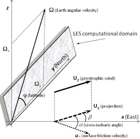
Fig. 1. The coordinate system used in this study with definitions

of the main vectors and angles. The orientation of the LES compu-tational domain is sketched by the shaded rectangle.xaxis points due east,yaxis points due north andzaxis is normal to the planet surface at given latitudeϕ.

2 Problem formulation

2.1 External control parameters

The Ekman boundary layer is controlled by three external parameters, namely the angular velocity of the frame ro-tation,  [s−1]; surface roughness, z0 [m]; and the hori-zontal pressure gradient, conveniently expressed through a geostrophic velocity of the free flow,Ug=(ρ0fV)−1z×∇p

[m s−1]. Here,ρ0 [kg m−3] is the constant fluid density,p

[kg m−1s−2] is the static pressure andϕis the latitude of the frame of reference. The local coordinate system is given by the orthogonal axes with the unit vectors:x– directed toward the east;y– directed toward the north; andz– directed nor-mal to the surface opposite to the gravity acceleration vector

g. The geostrophic wind speed is defined asG=Ug. The

angle between thex axis and the geostrophic velocity isβ. Figure 1 shows the coordinate system, the main vectors and the simulation domain.

2.2 Equations and internal EBL parameters

The EBL dynamics is governed by the incompressible Navier–Stokes equations

du

dt +(∇×u+fVz+fHy) ×u+∇ p

ρ0−∇(ν∇u)=0, (1)

divu=0. (2)

Here,u[m s−1] is the flow velocity andν [m2s−1] is the kinematic viscosity, which in the turbulent EBL is assumed to be an eddy viscosity. In the case of the horizontally ho-mogeneous steady-state flow, these equations admit the well-known Ekman stationary solution (e.g., D08),

u0(z+)=G (u0x+v0z)

u0 z+=cosβ−e−z

+

cos β−z+ v0 z+=sinβ−e−z

+

sin β−z+ z+=z

δ. (3)

This solution gives the Ekman depth scaleδ=√2_2ν/f

V [m]

as an internal length scale parameter. In the turbulent EBL above the viscous sublayer, scaling on the molecular kine-matic viscosity becomes irrelevant. In order to circumvent this problem,νshould be understood as an effective viscosity of the turbulent fluid (Muschinski, 1996; Z03; Esau, 2004a; D08), which is an integral parameter of the EBL only indi-rectly linked to the variable eddy viscosity in the turbulent flow.

The effective viscosity can be defined through the flux– gradient relationship in the following form

|τ| =u2_∗=νd|u|

dz =ν G

δ. (4)

The effective viscosity becomes

ν=u 2 ∗δ G =

2

fVG 2_C4

g. (5)

The Ekman depth scale will be expressed as

δ= 2u 2 ∗

fVG (6)

and will give a simple expression for an effective Reynolds number

Re=Gδ ν =

_G u∗

2

=C_g−2. (7)

The last equation relates the EBL bulk Reynolds number with a single internal turbulent parameter, namely with the fric-tion velocity u∗= |τ(z=0)|1/2. Stability analysis in D08 suggests that the EBL rolls are sensitive tofH atRe >300,

The above definitions are consistent with the behavior of the turbulence in the present LES. The reader should pay attention to the obtained reciprocal dependenceRe∝u−2_∗ . This dependence is known for the lowRe boundary layer flows whereReis based on the constant molecular kinematic viscosity. At molecularRe >103, the boundary layer under-goes transition to well-developed turbulence and the depen-dence becomes the direct proportionalityRe∝u∗. Thus, the introduced effectiveRe characterizes the EBL as a weakly turbulent boundary layer with respect to the most energetic eddies in the flow. As LES in this study show, the simulated EBL do not undergo transition to the fully chaotic state for effectiveRe <103, but such a transition does occur for ef-fectiveRe >103. Thus, this effectiveRecorrectly describes the EBL flow behavior. Dynamical reasons for such a behav-ior remain poorly understood; specifically, the relative role of the limited grid resolution versus energy concentration in large eddies is unclear.

2.3 The logarithmic law of the wall and resistance laws

The layer just above the surface where the turbulence is the most intensive is traditionally described as a constant flux layer in theoretical constructions and parameterizations. In this layer, which typically occupies 15 to 20 % of the turbu-lent EBL, the non-dimensional velocity gradient is

8=kz u∗

du

dz

, (8)

wherek is the von Karman constant. The non-dimensional gradient in the non-rotated EBL is linearly scaled with height, giving8=1. The EBL cannot be considered as a non-stratified layer due to the effect of the Coriolis stratifica-tion as described in Bradshaw (1969) and subsequent publi-cations (e.g., Esau, 2003). Galperin et al. (1989) introduced a stability correction compatible with the second order closure, which reads as

8=(1+CHξH)2+(CVξV)2 1/2

, (9)

where

ξH= z LH, ξV=

z

LV, (10)

LH= u∗ kfH

, LV= u∗ kfV

. (11)

This parameterization is not fully correct as it states that

fV always leads to 8 >1, which is incorrect for the EBL

in the Southern Hemisphere and would disagree with lab-oratory experiments (Nickels and Joubert, 2000). However, since|CV| |CH|for zonal winds, whereCV= −1.08 and CH=3.51 cosβ, and the presented LES runs were conducted

in the Northern Hemisphere, this problem does not affect this study. Equation (9) shows that8WE>1 in the EBL driven

by the flow from west to east (WE-EBL) and8EW<1 in

the EBL driven by the flow from east to west (EW-EBL). The difference|_8WE−8EW|increases toward the equator, in proportion to cosϕ. If the surface friction velocity is un-changed, which is not quite true as we will see later, the dif-ference at the equator could be estimated as

|8WE−8EW| =2

max β CH

_{2k z||}

u∗

∼0.35. (12)

Here, the following values are used:u∗=0.2 m s−1,k=0.4,

|| =7.29×10−5s−1,z=200 m. At the pole

8WE=8EW= 1+

CV

2k z|| u∗

2!1/2

∼ √

1+0.05=1.02>1. (13) At the pole the deviation from the expectation8=1 is too small to be firmly established from LES or observation data. Integration of Eq. (8) assuming8=1 gives the integral form of the law of the wall

u∗=k|u(z)|

ln_zz 0

. (14)

Then the resistance laws could be written as

A=ln CRCgRo− κ

Cgcosα, (15) B= − κ

CRCg

sinα, (16)

where Ro=G(fVz0) is the roughness Rossby number

(Zilitinkevich and Esau, 2005; Esau and Zilitinkevich, 2006). The non-dimensional parameter

CR=hPBLfVu∗ (17)

estimates the depth of the essentially turbulent EBL (Rossby and Montgomery, 1935; Zilitinkevich et al., 2007). Empirical evidence shows thathPBLδ, which is also true for these

LES.

Published studies have considered the EBL structure at the pole, as in Ekman (1905). Therefore, changes in the internal EBL parametersA, BandCRat lower latitudes were over-looked, as they were expected to be constants with the same values as atϕ=90◦N. As we will see here, these parame-ters depend on bothϕ andβ, which suggests a dependence onfH.

2.4 Instability of the stationary Ekman solution

0 5 10 15 20 0

500 1000 1500 φ = 1

o_N

time (hours)

Re

0 5 10 15 20

0 500 1000 1500 φ = 5

o_N

time (hours)

Re

0 5 10 15 20

0 500 1000 1500 φ = 15

o_N

Re

0 5 10 15 20

0 500 1000 1500 φ = 30

o_N

Re

0 5 10 15 20

0 500 1000 1500 φ = 45

o_N

Re

0 5 10 15 20

0 500 1000 1500 φ = 60

o_N

Re

0 5 10 15 20

0 500 1000 1500 φ = 75

o_N

Re

0 5 10 15 20

0 500 1000 1500 φ = 90

o_N

Re

(a)

0 0.2 0.4 0.6 0.8 1 1.2 1.4 1.6 1.8 2 −0.01 0 0.01 0.02 0.03 0.04 0.05 0.06 0.07 0.08 0.09 1o_N

5o_N

15o_N

30o_N

45o_N

60o_N 75o_N

90o_N

f v × 10

4

Cg

(b)

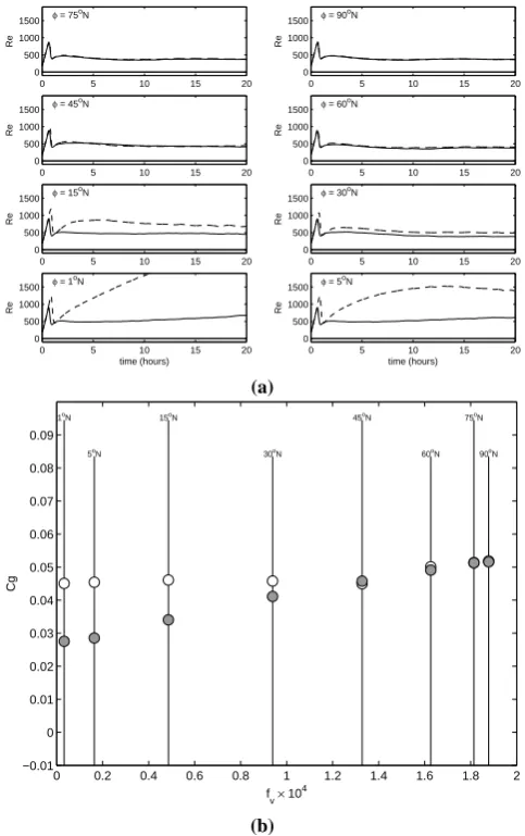
Fig. 2. The geostrophic drag coefficientCg=u∗/G: (a) time evo-lution of the effectiveRe=Cg−2 (solid curves are for EW-EBL; dashed curves are for WE-EBL); (b) values of the coefficient at hour six of the LES integration. Shaded circles show the WE-EBL; open circles, the EW-EBL.

rolls. This set of instabilities could affect the EBL parameters in a way unaccounted for by the Reynolds stress equations. The impact is related to selective growth of certain turbulent scales, which is not reflected in the corresponding changes of the turbulent dissipation. The cross-flow length scale of the fastest growing mode of the rolls islroll=4π δ≈π hEBL

with a non-dimensional growth rateσ1=0.024 atRe >500. D08 mentioned that this growth rate should be considered as a function of the flow Reynolds number and the rotational stability parameters; that is,σ1=σ1(Re, ξV, ξH). Such a

the-oretical analysis has been done for some combinations of pa-rameters, but the general picture is still missing. The analysis in D08 shows that the rolls grow during the initial stage for

t=10 δGσ1∼6 h. This stage is followed by the

satu-ration stage. AtRe >1000, the rolls do not saturate and, as

we will show, they are destroyed by the secondary instability. The saturated roll stage was of primary interest in the earlier LES studies; for example, Z03 investigated the EBL structure after 416 h of the model run time.

3 Results

3.1 Concept of numerical experiments

This study addresses the impact of the EBL structures dur-ing the growdur-ing and stationary stages of their development. Therefore, it was important to make the simulation domain sufficiently large in the cross-flow direction for undisturbed development of a statistically significant number of rolls. The longitudinal dimension along thex axis was designed to be only eight grid points (0.28125 km), whereas the cross-flow dimension along theyaxis was 4096 grid points (144.0 km). The small size of the longitudinal dimension is sufficient to resolve the fastest growing mode of the expected secondary instability (D08). It is also sufficient for the dynamic-mixed turbulence closure in the model to work. The vertical dimen-sion alongzaxis was 128 grid points (3.0 km). The height of the domain is sufficient to accommodate the stationary EBL at latitudes poleward of 30◦N. At lower latitudes, the EW-EBL comprised the whole domain by the sixth hour of model integration and therefore its further evolution was affected by this constraint.

The LESNIC runs are listed in Table 1. The runs were driven with the westerly (β=0◦, therefore denoted as WE-EBL in Table 1) and easterly (β=180◦_{, EW-EBL in}

Ta-ble 1) geostrophic winds with the speedG=5 m s−1. The runs were conducted in the “f plane” at eight different lat-itudes from 1 to 90◦N. Except for the geostrophic wind di-rection and the run’s latitude, the other parameters were kept the same for all experiments. Surface roughness was set to

z0=0.1 m. The grid resolution was 35.15 m in the

horizon-tal dimensions and 23.43 m in the vertical dimension. Each run was integrated over 22 model hours with sam-pling of the horizontally averaged turbulence and mean flow statistics every 60 s and storage of the full three-dimensional fields of the model velocity at the end of each model hour. The resulting simulation database provides information for the study of the time evolution of the EBL structures and pa-rameters as well as for the statistical study of the EBL struc-tures in their development.

Table 1. Parameters of the large-eddy experiments with LESNIC. Internal EBL parameters are given at the sixth hour of integration.

Run Case Latitude,ϕ u∗[m s−1] α[deg] Re hPBL[m] δ[m] CR A B k 8 h|9|iy

LES runs in large 144 km domain

WE U5L1 WE-EBL 1◦N 0.138 1.8 1300 360 480 0.007 −2.9 50.4 0.31 1.00 0.22 EW U5L1 EW-EBL 1◦N 0.225 0.4 490 2270 403 0.026 1.0 2.4 0.41 0.56 9.70 WE U5L5 WE-EBL 5◦N 0.143 8.3 1230 380 220 0.034 −2.8 46.9 0.32 1.12 0.35 EW U5L5 EW-EBL 5◦N 0.227 2.8 490 2450 175 0.137 1.1 3.2 0.41 0.56 8.37 WE U5L15 WE-EBL 15◦N 0.170 18.4 860 560 130 0.123 −0.9 25.6 0.34 1.33 1.73 EW U5L15 EW-EBL 15◦N 0.230 7.9 470 2570 99 0.420 1.3 2.9 0.41 0.56 9.51 WE U5L30 WE-EBL 30◦N 0.206 22.6 591 720 92 0.260 1.0 12.9 0.35 1.39 4.32 EW U5L30 EW-EBL 30◦N 0.230 16.5 480 1850 71 0.600 1.6 4.1 0.40 0.69 12.7 WE U5L45 WE-EBL 45◦N 0.229 23.7 480 630 82 0.280 1.7 10.9 0.35 1.23 8.23 EW U5L45 EW-EBL 45◦N 0.225 15.2 500 1100 70 0.510 1.4 4.3 0.38 1.04 5.77 WE U5L60 WE-EBL 60◦N 0.245 23.2 420 580 74 0.300 2.2 9.4 0.35 1.13 7.75 EW U5L60 EW-EBL 60◦N 0.251 21.9 400 710 76 0.360 2.2 7.5 0.36 1.10 8.12 WE U5L75 WE-EBL 75◦N 0.256 21.9 380 560 74 0.330 2.3 7.7 0.35 1.10 6.61 EW U5L75 EW-EBL 75◦N 0.257 21.7 380 580 75 0.318 2.3 7.9 0.35 1.06 7.30 WE U5L90 WE-EBL 90◦N 0.258 21.8 370 540 74 0.310 2.4 8.1 0.35 1.06 6.12 EW U5L90 EW-EBL 90◦N 0.259 21.5 380 580 73 0.328 2.4 7.5 0.35 1.06 9.81

LES runs in small 1.225 km domain

WE U5L5 WE-EBL 5◦N 0.136 11.2 1360 420 210 0.039 −7.9 82.6 0.45 0.98 0.25 EW U5L5 EW-EBL 5◦N 0.197 3.4 640 2310 210 0.149 −0.5 4.9 0.42 1.07 2.63 WE U5L90 WE-EBL 90◦N 0.259 21.9 370 420 74 0.240 0.8 15.0 0.43 0.93 0.85 EW U5L90 EW-EBL 90◦N 0.257 24.5 380 380 75 0.216 0.9 15.4 0.41 0.71 0.69

3.2 Turbulent surface drag and effective Reynolds

number

We begin the discussion of the LES results with consider-ation of the key internal parameter – the turbulent surface drag or the surface friction velocityu∗. Figure 2 reveals that in terms ofReboth EW-EBL and WE-EBL reach the station-ary stage at high latitudes whereRe≈500 (as expected for the environmental EBL) andu∗≈0.22 m s−1. The WE-EBL at lower latitudes behaves differently. In these runs,Re in-creases for a longer period, and reaches much larger values. The Reynolds number is approximately 1000 at 5◦N. This corresponds to roughly 30 % of the turbulent stress reduction as compared to the EW-EBL at the same latitude. Smalleru∗

andCgindicate reduced vertical momentum transport. This difference is larger than obtained in the Reynolds stress anal-ysis of Galperin et al. (1989), but much smaller than found in the LES of tidal flow by Salon and Armenio (2011).

3.3 The depth of the turbulent EBL

We define the depth of the essentially turbulent EBL,

hPBL, as the height where the magnitude of the turbulent

stress drops to 5 % of its surface value; that is, hPBL: |τ(z=hPBL)| =0.05u2∗. Similarly, one can define the depth

of the weakly turbulent layer as h1_PBL: τ(z=h1_PBL)=

0.01u2_∗and the depth of the strongly turbulent layer ash10_PBL:

τ(z=h10_PBL)=0.10u2_∗. These three thresholds are shown

in Figs. 8–11 in this study. Previous studies have overlooked

thathPBLand particularly the depth of the weakly turbulent

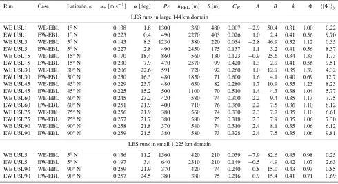
layer,h1_PBL, should be sensitive to the rolls, which are found in the upper part of the EBL. Figure 3 shows that the turbu-lent EW-EBL becomes deeper than the WE-EBL by 60◦N. Unfortunately, the LES domain was not sufficiently deep to accommodate the stationary EW-EBL at latitudes lower than 30◦N. Nevertheless, the faster growth of the EW-EBL depth is clearly seen in the early stages of the EBL development.

The development of the rolls in the EW-EBL has a pro-found impact on the EBL depth with a much deeper turbu-lent layer at low latitudes. This increase (by almost one order of magnitude) is not fully reflected in the surface stress and in the effective eddy viscosity, and therefore, in the Ekman scale and in the Rossby–Montgomery parameter, CR. Zil-itinkevich et al. (2007) reviewed estimations ofCR in pub-lished LES and DNS studies, as well as our own simulations with LESNIC to suggest the best fit ofCR=0.65±0.05. The new simulations, whereCRwas somewhat lower than in the fully three-dimensional simulations, show that this fit is valid only for latitudes poleward of 45◦N. Figure 3c shows the pa-rameterCR1, which characterizes the depth of the weakly

turbulent layer, as it more correctly reflects the impact of the rolls on the EBL. Values ofCRandCR1decrease at low

lat-itudes (Table 1), being just around 0.1 at 5◦_{N, highlighting}

0 5 10 15 20 0

0.5 1

φ = 1oN

time (hours) hPBL

+

0 5 10 15 20

0 0.5 1

φ = 5oN

time (hours) hPBL

+

0 5 10 15 20

0 0.5 1

φ = 15o_N

hPBL

+

0 5 10 15 20

0 0.5 1

φ = 30o_N

hPBL

+

0 5 10 15 20

0 0.5 1

φ = 45o_N

hPBL

+

0 5 10 15 20

0 0.5 1

φ = 60o_N

hPBL

+

0 5 10 15 20

0 0.5 1

φ = 75o_N

hPBL

+

0 5 10 15 20

0 0.5 1

φ = 90o_N

hPBL

+

(a)

0 0.2 0.4 0.6 0.8 1 1.2 1.4 1.6 1.8 2 0 0.1 0.2 0.3 0.4 0.5 0.6 0.7 0.8 0.9 1 1o N

5oN 15o

N

30oN 45o

N

60oN 75o

N

90oN

f_v× 104 hPBL

+

(b)

0 0.2 0.4 0.6 0.8 1 1.2 1.4 1.6 1.8 2 0 0.1 0.2 0.3 0.4 0.5 0.6 0.7 0.8 0.9 1 1oN

5oN 15oN

30oN

45oN

60oN 75oN

90oN

fv× 10 4 CR1

(c)

Fig. 3. The depth of the essentially turbulent EBL: (a) time

evolu-tion of the non-dimensional depthh+_EBL=hEBLLz, whereLz=

3 km is the vertical size of the LES domain (solid curves are for EW-EBL; dashed curves are for WE-EBL); (b) values ofh+_EBL

at hour six of the LES integration; and (c) values of the Rossby– Montgomery parameterCR1for the weakly turbulent EBL at hour six of the LES integration. Shaded circles show the WE-EBL; open circles, the EW-EBL.

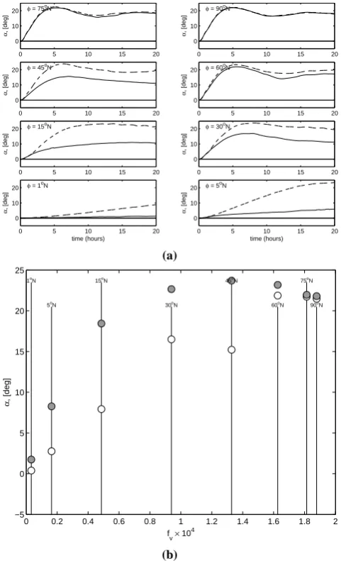
3.4 The cross-isobaric angle

The cross-isobaric angle defines several important phenom-ena (Svensson and Holtslag, 2009). Since this angle is de-termined by the balance between the turbulent friction and the pressure gradient, its value is sensitive to the depth of the EBL and to the vertical distribution of the eddy viscosity. In the turbulent EBL,α≈19◦at the pole (Coleman, 1999; Esau, 2004a; Marlatt et al., 2012), which is defined fromfV

in the Ekman solution in Eq. (3). This angle increases in shal-lower layers and decreases in deeper layers (Esau and Zil-itinkevich, 2006). Figure 4 shows that the deeper EW-EBL haveαreduced to about 5◦at 15◦N, whereas the shallower WE-EBL still haveα≈20◦ at this latitude. It directly fol-lows from Eq. (3) thatαshould decrease toward the equator, which is observed in the LES data.

3.5 The resistance laws

The observed changes in the surface friction velocity, the cross-isobaric angle and the EBL depth do not compensate each other in the resistance laws. Hence, they should modify the parametersAandB of the resistance laws in Eqs. (15) and (16). When Zilitinkevich and Esau (2005) revisited the resistance laws, they focused on the effect of the stable strat-ification but overlooked the effects of the Coriolis stratifica-tion. This gave a formulation of the neutral limit of the resis-tance laws through variables

mA=Cf ACR, mB=Cf BCR, (18) where the constantsCf A=Cf B=1. The proposed analyti-cal resistance law approximations read

A= −amA+ln(a0+mA) , (19)

0 5 10 15 20 0

10 20 φ = 1o_N

time (hours)

α

, [deg]

0 5 10 15 20

0 10 20 φ = 5o_N

time (hours)

α

, [deg]

0 5 10 15 20

0 10 20 φ = 15oN

α

, [deg]

0 5 10 15 20

0 10 20 φ = 30oN

α

, [deg]

0 5 10 15 20

0 10 20 φ = 45oN

α

, [deg]

0 5 10 15 20

0 10 20 φ = 60oN

α

, [deg]

0 5 10 15 20

0 10 20 φ = 75oN

α

, [deg]

0 5 10 15 20

0 10 20 φ = 90oN

α

, [deg]

(a)

0 0.2 0.4 0.6 0.8 1 1.2 1.4 1.6 1.8 2 −5 0 5 10 15 20 25 1o_N

5o_N

15o_N

30o_N

45o_N

60o_N 75o_N

90o_N

f v× 10

4

α

, [deg]

(b)

Fig. 4. The cross-isobaric angle in the EBL: (a) time evolution (solid

curves are for EW-EBL; dashed curves are for WE-EBL); (b) values ofαat hour six of the LES integration. Shaded circles show the WE-EBL; open circles, the EW-EBL.

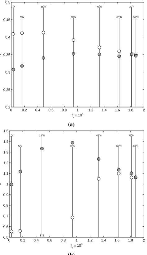
3.6 Non-dimensional velocity gradient in the constant

flux layer

Calculation of the non-dimensional velocity gradients,8, in the LES meets certain difficulties given that the von Karman constant,k=0.4, as prescribed at the first model level, does not necessarily have a value consistent with the simulated turbulence. We redirect the reader to ¨Osterlund et al. (2000) for a more detailed discussion on the von Karman constant values. Therefore, as the first step, the consistent value ofk

should be recovered. This is done using Eq. (14) with averag-ing of the obtainedkover the lowest 15 % of the essentially turbulent EBL. These values of the von Karman constant are shown in Fig. 6a. The non-dimensional velocity gradients were calculated at each level using this constantk(Fig. 6b),

0 0.2 0.4 0.6 0.8 1 1.2 1.4 1.6 1.8 2 −5 −4 −3 −2 −1 0 1 2 3 4 5 1o_N

5o_N

15o_N

30o_N

45o_N

60o_N 75o_N

90o_N

f v× 10

4

A

(a)

0 0.2 0.4 0.6 0.8 1 1.2 1.4 1.6 1.8 2 −2 0 2 4 6 8 10 12 14 16 18 20 1o_N

5oN

15o_N

30oN

45o_N

60oN 75o_N

90oN

f v× 10

4

B

(b)

Fig. 5. The parametersA(a) andB(b) of the resistance laws in the

EBL. The solid curve is the analytical approximations withhPBL andαfor the WE-EBL (dashed line) and the EW-EBL (solid line). Shaded circles show the WE-EBL; open circles, the EW-EBL. The data correspond to hour six of integration.

and then averaged over the same fraction of the EBL. This procedure has proved to be robust for identification of the logarithmic regions in the velocity profiles, and is often used in analysis of laboratory experiments ( ¨Osterlund et al., 2000; Nickels and Joubert, 2000).

The non-dimensional velocity gradient (8=1.03 in LES) corresponds well with our ad hoc estimation (8=1.02 in Eq. 13) for the pole. Similarly, the difference|8WE−8EW| =

0.4–0.8 at low latitudes is in good agreement with the esti-mation of 0.35 from Eq. (12). This agreement is surprising as changes in8due tofH effects and the EBL structuring

0 0.2 0.4 0.6 0.8 1 1.2 1.4 1.6 1.8 2 0.2

0.25 0.3 0.35 0.4 0.45 0.5 1o_N

5o_N

15o_N

30o_N

45o_N

60o_N 75o_N

90o_N

f_v× 104

κ

(a)

0 0.2 0.4 0.6 0.8 1 1.2 1.4 1.6 1.8 2 0.5

0.6 0.7 0.8 0.9 1 1.1 1.2 1.3 1.4 1.5 1o_N

5o_N

15o_N

30o_N

45o_N

60o_N 75o_N

90o_N

f v× 10

4

Φ

(b)

Fig. 6. The non-dimensional velocity profile: (a) the von Karman

constantkin LES averaged over the lowest 15 % of the EBL; (b)

8computed with thiskand averaged over the same fraction of the EBL. Shaded circles show the WE-EBL; open circles, the EW-EBL. The data correspond to hour six of integration.

parameters. The presented LES show that those changes are significant, and even large (e.g., inhPBL), whereas Galperin

et al. (1989) and subsequent publications invoking the anal-ysis of the Reynolds stress model maintain that the effect should be small. Nevertheless, as for8, the LES results and the model analysis seem to be in agreement.

4 Discussion

4.1 The impact of rolls on the EBL parameters

A question may be asked about the impact of rolls – i.e., the large-scale, self-organized structures in the EBL – on the observed dependences of the internal EBL parameters on the wind direction and latitude. On the one hand, the Reynolds stress equations, such as in the second-order clo-sure by Galperin et al. (1989), do not account for instability and selective growth of turbulent perturbations with a cer-tain structure. Nevertheless, some parameters, e.g., the non-dimensional velocity gradient, derived from those equations, are in good correspondence to the LES results. On the other hand, the EBL stability analysis in D08, which attributes the dependences to restructuring of the EBL, is also consistent with the LES results, including the instant flow visualiza-tions in terms of the anomalous velocity and stream func-tion. Esau (2004b) attempted to estimate this effect by ap-plying constraints on the EBL depth, which would constrain the size of the largest eddies in the boundary layer. The EBL depth was constrained through imposed stable stratification. Significant effect was found but the size of the LES domain was not sufficiently large to firmly establish the effect.

D08 quoted at least two possible dynamical mechanisms for the Coriolis force to impact the EBL parameters. It may act indirectly through modification of the Reynolds stress component reserving some fraction of the turbulent kinetic energy E=0.5u02_+v0₂

+w02 _{in the cross-flow}

veloc-ity fluctuationsv02_{, which are otherwise much less intense.}

The energy in the longitudinal velocity fluctuations u02 _is

quickly replenished in the sheared flow. Hence, this mecha-nism is important in the strongly-sheared constant-flux layer, where LES and Reynolds stress equation analysis are in good correspondence. The horizontal Coriolis force component,

fH, also modifies the domain of the primary instability of

the flow directly (Leibovich and Lele, 1985), but this effect should be small atRe∼500, as found in LES. Instead,fH

acts through the secondary instability, which stabilizes or destabilizes the rolls depending on the mean flow direction and latitude. Since the rolls are dominant structural features in the weakly turbulent layer in the upper part of the EBL, their stabilization or destabilization should have a major im-pact on the EBL depth and related parameters.

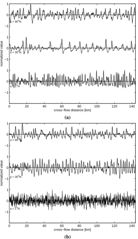
Figure 7 shows quasi-regular alternations of the instant in-tegrated vertical velocity component

w+(γ , ϕ, β)= hwi_x,z/maxhwi_x,z (21) at hour six of the simulations. The angular brackets h i_x,z

0 20 40 60 80 100 120 140 −1

0 1 −1 0 1 −1 0 1

φ = 1oN φ = 30oN φ = 90oN

cross−flow distance [km]

normalized value

(a)

0 20 40 60 80 100 120 140

−1 0 1 −1 0 1 −1 0 1

φ = 1o_N

φ = 30oN φ = 90oN

cross−flow distance [km]

normalized value

(b)

Fig. 7. The instant cross-flow fluctuations of the vertical velocity

component integrated alongzand xaxes at the end of the linear growth stage at the hour six of the LES run. The fluctuations are shown for latitudes 90◦N, 30◦N and 1◦N in the EW-EBL (a) and WE-EBL (b). The values are normalized by the maximum value at each latitude. The positive values correspond to upward motions.

flow. Although the alternation pattern is similar at the pole, it becomes rather different at low latitudes where the velocity alternation scales in the EW-EBL are noticeably larger and more skewed than in the WE-EBL.

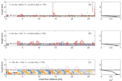
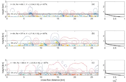
We visualize the first 27 km of the LES domain alongy

(meridional) direction. The structure of the EBL is shown through the secondary flow stream function (contours) and longitudinal velocity anomalies (color shading) in Figs. 8– 11. These figures also include the vertical profiles of the aver-aged vertical momentum fluxh|τ|i_xy. The velocity anomaly is defined as

u0(y, z)= hu(x, y, z)i_x− hu(x, y, z)i_x,y. (22) The stream function is defined following D08 as

9:v0= −∂9

∂z, w0=∂9

∂z. (23)

Except for the WE-EBL at low latitudes, the closed circu-lation contours are clearly observed in these figures. These contours identify the rolls in the EBL with both the most intensive roll circulations (the largest amplitude |9|of the stream function) and the largest spatial scales of the rolls, found in the EW-EBL at low latitudes. Centers of the roll cir-culation are located in the upper part of the EBL atzδ∼3– 4, which is consistent with theoretical analysis.

The closed stream function contours are located in the weakly turbulent layer, as comparison with the momentum flux profile confirms. Further analysis found high correlation (corr. coef. 0.6) betweenh|9|i_y and the EBL depth. Thus, the rolls are essentially a feature of the upper EBL. The observed roll length scale is lroll=4π δ≈π hPBL≈ 3 km.

We conducted four additional LES runs in a horizontally restrictive domain, Ly=0.5hPBL(ϕ=5◦N)=1225 m

(Ta-ble 1), to prevent development of the rolls at the most un-stable mode. It was expected that without the rolls, the WE-EBL and EW-WE-EBL at low latitudes would exhibit less dif-ferent values of the internal parameters. This is, however, not the case. Figure 12 shows stream functions and veloc-ity anomalies of four LES runs. As Fig. 12c and d show, the rolls constrained by the LES domain are organized in a two-level structure where the size of rolls at each two-level fits the size of the domain. This explains the success of earlier simu-lations with too restrictive domains (Mason and Sykes, 1980; Z03). This result follows from the continuity of the spectrum of unstable modes in the EBL. If the most unstable mode does not fit into the LES domain, a circulation pattern con-sistent with the largest allowed unstable mode develops. By the other words, the instability amplifies the largest mode re-solved in the domain. Thus, we are not able to resolve ambi-guity around the role of the rolls in the EBL. However, these experiments suggest that the rolls have an impact on the EBL indirectly through modification of the EBL depth and subse-quent change of parameters, which depend on the EBL depth.

4.2 The secondary instability of rolls

At lower latitudes, the characteristics of the WE-EBL and the EW-EBL become increasingly different, suggesting that the control offHshould be sensitive to the wind directionβ.

There are two mechanisms of thefHcontrol described in the

Fig. 8. Cross-flow sections (yzplanes) of the instant flow patterns in WE-EBL at 5◦N. The patterns are given at the beginning (after 3 h of LES integration at the upper panel) and the end (after 6 h at the middle panel) of the linear growth stage as well as for the quasi-stationary stage (after 18 h at the bottom panel). Contours represent the anomalies flow stream function from Eq. (30), with negative values shown as dashed contours. The color shading represents the anomalous flow velocity from Eq. (29), with blue corresponding to the slow motions. The time of the snapshots, the EBLReat that time and the range of the stream function values are indicated on the panels. The horizontal lines show the EBL depthsh10_PBL(the lowest line),hPBLandh1PBL(the highest line).

this mechanism. The present LES demonstrated that both the EBL depth and the turbulence length scales are consistently decreasing in the WE-EBL from the pole, where this mech-anism is inactive, toward the equator, where this mechmech-anism is supposed to be responsible for the structuring of the flow. The weak but still growing rolls are not observed in the sim-ulations.

Another mechanism is secondary instability of the rolls, which becomes increasingly active at Re >300. This in-stability perturbs the rolls in the longitudinal direction. But its growth rate,σ2, over the range of length scales

permit-ted in the LES domain, depends onβ. D08 analysis for the maximum permitted LES length scale in the zonalx direc-tion (the minimum wave number k2=2.7, latitude 45◦N andRe=500)gives the non-dimensional growth rates equal toσ₂WE= +0.005 andσ₂EW= −0.005. It suggests roll sta-bilization in the EW-EBL and destasta-bilization, albeit only weakly, in the WE-EBL. The simulated EBL evolution sug-gests that there might be a run-away loop of roll destabi-lization in the WE-EBL. The initially weak destabidestabi-lization reduces the roll circulation and decreases the momentum transport in the EBL. This raises the effectiveRe∝1

u2_∗

of the flow, making the rolls more unstable with respect to the secondary instability. These more unstable modes further

destabilize the rolls, raiseRe and then destabilize the rolls even more. The S-shaped colored structures in the velocity anomalies between the weak rolls are observable in Fig. 8c. These structures are similar to the velocity structures respon-sible for the secondary instability in D08.

The destructive secondary instability counteracts the pri-mary instability in the EBL. The later one is, however, stronger; that is, their growth rates relate asσ1>σ2. Hence,

weak and strongly perturbed rolls emerge slowly even in the WE-EBL at latitudes larger than 5◦N. Detailed examination of the LES results at 1◦N reveals a qualitatively different scenario. In close vicinity to the equator, the rolls do not emerge, leaving the WE-EBL in a chaotic state. This is prob-ably the effect of suppression of redistribution between lon-gitudinal and vertical components in the turbulent stress as it follows from the Reynolds stress equations. This effect has been noted in Z03 and appeared in these LES as well.

5 Conclusions

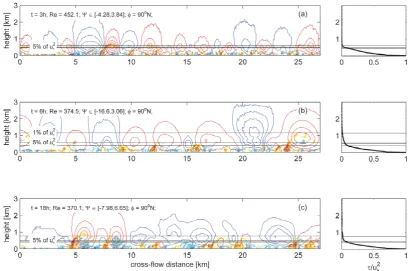
Fig. 9. Cross-flow sections (yzplanes) of the instant flow patterns in EW-EBL at 5◦N. The panels are composed similarly to Fig. 8.

Fig. 11. Cross-flow sections (yzplanes) of the instant flow patterns in EW-EBL at 90◦N. The panels are composed similarly to Fig. 8.

similar to those roll structures that have been previously found in analytical studies of the EBL instabilities. If our def-inition of the effectiveReof the EBL is accepted, then not only the qualitative structure of the rolls but also their quanti-tative characteristics (such as the cross-flow length scale, the growth rate and sensitivity to the secondary instability), are in good correspondence with the proposed EBL theory.

The rolls are found in both the WE-EBL and the EW-EBL at high latitudes. The structures of both boundary layers are nearly identical at high latitudes, but the difference between them gradually increases toward the equator. At low lati-tudes, the rolls in the EW-EBL quickly grow, and by hour six of simulations occupy the entire LES domain. They maintain the strong vertical momentum transport and surface stress, keeping the effectiveReat about 500. The rolls in the WE-EBL evolve slowly, experiencing destabilization from the secondary instability and suppression of the momentum re-distribution by the Coriolis force. The difference between the EW-EBL and the WE-EBL was found to be the largest by hour six of simulations.

The previously published analyses of the Reynolds stress equations (e.g., Galperin et al., 1989) concluded that the im-pact of the horizontal component of the Coriolis force,fH,

on the internal EBL parameters is rather small. The theoret-ical studies of the EBL structures (e.g., Etling and Brown, 1983; D08) have not come to a certain conclusion on this point. These LES revealed that the impact of fH and the

corresponding differences in the EBL structure is significant. The LES results are consistent with theoretical estimations in the constant flux layer. At the same time, the LES show large changes in the EBL depth and the structure of the upper EBL due to the effects offH. At low latitudes (below 30◦N), the

turbulent EW-EBL is 3–5 times deeper than the WE-EBL. Correspondingly, the internal EBL parameters, which are sensitive to the EBL depth (the Rossby–Montgomery param-eter, the cross-isobaric angle, the resistance law constants), also show sensitivity to the wind direction and latitude, con-firming the results in Esau (2012).

Fig. 12. Cross-flow sections (yzplanes) of the instant flow patterns in four LES runs: (a) WE U5L5 and (c) WE U5L90 in the small LES domain; (b) WE U5L90 and (d) WE U5L90 in the large LES domain. The panels are composed similarly to Fig. 8.

Appendix A

Large-eddy simulation model LESNIC

This study uses the Large Eddy Simulation Nansen Cen-ter Improved Code (LESNIC) of Esau (2004a). LESNIC has been used in other studies by the authors as well as in the large-eddy simulation intercomparison experiments (Beare et al., 2006). LESNIC solves the equations of mo-tions for incompressible Boussinesq fluid. The model equa-tions are given by the system equaequa-tions (1) and (2), where the turbulent stress termτ =ν∇uis parameterized through a dynamic-mixed turbulence closure (DMC).

The DMC eliminates the problem of excessive turbulent eddy viscosity in the LES noted in earlier works (e.g., An-dren et al., 1994; Beare et al., 2006). It raises the effective

Reof simulations and better reproduces the law of the wall in the constant flux layer as demonstrated by Porte-Agel (2000), Esau (2004a) and Glazunov (2009). The DMC (Germano et al., 1991; Zang et al., 1993) exploits universal scaling of the energy spectrum in the inertial sub-range of scales where the spectral energy flux is a universal function of wave number. It leads to the so-called Germano equality, which links

tur-bulent stresses on two different scales within the universal interval of scales. The scales are defined by the filtering op-erators denoted as ()L and()l, where the filter widths are

1L> 1land both scales are within the inertial sub-range of scales. Vreman (1997) showed that one can obtain the fol-lowing equations:

τij =LLij−2ls2 Sij

Sij, (A1)

l_s2=1

2

h(LL_ij−H_ijL)M_ijLi_ij

hM_ijLM_ijLi_ij . (A2)

Here, the angular brackets denote averaging over alli, j=

1,2,3 tensor components. Furthermore, to stabilize the model, the variability of the Smagorinsky length scale is lim-ited to 0.01< ls<0.3. The tensors in Eqs. (24) and (25) are

H_ijL=

uL_iuL_jl

L −

uL_il L

uL_jl

L −

−

ul_i

L ul_j

L

−ul_iul_j

L

Here, square brackets are used only to group the terms. Fi-nally, the shear tensors are

Sij = 1 2

_∂u

i

∂xj

+∂uj ∂xi

M_ijL= Sij

Sij

L

−αL_l S

L ij

S

L

ij. (A4)

In these equations, variables without superscripts denote the quantities defined on the model grid. The filter width1l is taken equal to the grid size in the model, while the width

1L=21l. Such a combination givesα_lL=2.92. This is not an optimal choice of filters (Glazunov, 2009), but it is a rea-sonable trade-off between the quality and the speed of calcu-lations.

The surface boundary conditions in LESNIC are given by the law of the wall in Eq. (14) wherek=0.4. Free-slip boundary conditions are used at the top of the domain

τ=0, ∂u

∂z=0. (A5)

The numerical schemes in the model were described in Esau (2004a). LESNIC uses the second-order, fully conser-vative, finite-difference, skew-symmetric scheme; the uni-form staggered C-type mesh; and the explicit Runge–Kutta fourth-order time scheme. The LESNIC domain is periodic inxandydirections, which allows for application of the di-rect solving method for the Laplace equation for the dynamic pressure.

Acknowledgements. The research leading to these results has

received funding from the Norwegian Research Council projects PBL-feedback 191516/V30 and RECON 200610/S30; the Euro-pean Research Council Advanced Grant, FP7-IDEAS, 227915; and by a grant from the Government of the Russian Federation under contract No. 11.G34.31.0048. The authors acknowledge fruitful discussions with, and support from, A. Glazunov (Institute for Nu-merical Mathematics, Moscow, Russia) and J. Fricke (Institute for Meteorology and Climatology at Leibniz University in Hannover, Germany). The Norwegian program NOTUR provided necessary computer resources for calculations.

Edited by: Y. Troitskaya

Reviewed by: A. S. Petrosyan and two anonymous referees

References

Andren, A. and Moeng, C.-H.: Single-point closures in a neutrally stratified boundary layer, J. Atmos. Sci., 50, 3366–3379, 1993. Andren, A., Brown, A. R., Graf, J., Mason, P. J., Moeng, C.-H.,

Nieuwstadt, F. T. N., and Schumann, U.: Large-eddy simulation of a neutrally stratified layer: A comparison of four computer codes, Q. J. Roy. Meteorol. Soc., 120, 1457–1484, 1994. Ayotte, K. W., Sullivan, P. P., Andr´en, A., Doney, S. C., Holtslag, A.

A. M., Large, W. G., McWilliams, J. C., Moeng, C.-H., Otte, M. J., Tribbia, J. J., and Wyngaard, J. C.: An evaluation of neutral and convective planetary boundary-layer parameterizations rela-tive to large eddy simulations, Bound.-Lay. Meteorol., 79, 131– 175, 1996.

Beare, R. J., MacVean, M. K., Holtslag, A. A. M., Cuxart, J., Esau, I., Golaz, J.-C., Jimenez, M. A., Khairoutdinov, M., Kosovic, B., Lewellen, D., Lund, T. S., Lundquist, J. K., McCabe, A., Moene, A. F., Noh, Y., Raasch, S. and Sullivan, P.: An intercomparison of large-eddy simulations of the stable boundary layer, Bound.-Lay. Meteorol., 118, 247–272, 2006.

Bradshaw, P.: The analogy between streamline curvature and buoy-ancy in turbulent shear flow, J. Fluid Mech., 36, 177–191, 1969. Brown, R. A.: A secondary flow model for the planetary boundary

layer, J. Atmos. Sci., 27, 742–757, 1970.

Caldwell, D. R., van Atta, C. W., and Helland, K. N.: A laboratory study of the turbulent Ekman layer, Geophys. Fluid Dyn., 3, 125– 160, 1972.

Chereshkin, T. K.: Direct evidence for an Ekman balance in the Californian Current, J. Geophys. Res., 100, 18261–18269, 1995. Coleman, G. N.: Similarity statistics from a direct numerical simu-lation of the neutrally stratified planetary boundary layer, J. At-mos. Sci., 56, 891–900, 1999.

Dubos, T., Barthlott, C., and Drobinski, P.: Emergence and sec-ondary instability of Ekman layer rolls, J. Atmos. Sci., 65, 2326– 2342, 2008.

Ekman, V. W.: On the influence of the Earth’s rotation on ocean currents, Arkiv for Matematik, Astronomi och Fysik, 2, 1–52, 1905.

Esau, I.: Coriolis effect on coherent structures in planetary boundary layers, J. Turbulence, 17, doi:10.1088/1468-5248/4/1/017, 2003. Esau, I.: Simulation of Ekman boundary layers by large-eddy model with dynamic mixed sub-filter closure, Environ. Fluid Mech., 4, 273–303, 2004a.

Esau, I.: An improved parameterization of turbulent exchange coef-ficients accounting for the non-local effect of large eddies, Ann. Geophys., 22, 3353–3362, 2004b,

http://www.ann-geophys.net/22/3353/2004/.

Esau, I.: Large scale turbulence structure in the Ekman boundary layer, Geofizika, 29, 5–34, 2012.

Esau, I. N. and Zilitinkevich, S. S.: Universal dependences between turbulent and mean flow parameters instably and neutrally strat-ified Planetary Boundary Layers, Nonlin. Processes Geophys., 13, 135–144, doi:10.5194/npg-13-135-2006, 2006.

Etling, D. and Brown, R. A.: Roll vortices in the planetary boundary layer: A review, Bound.-Lay. Meteorol., 65, 215–248, 1993. Faller, A. J.: An experimental study of the instability of the laminar

Ekman boundary layer, J. Fluid Mech., 15, 560–576, 1963. Fricke, J.: Coriolis instabilities in coupled atmosphere-ocean

Holt, T. and Raman, S.: A review and comparative evaluation of multi-level boundary layer parameterizations for first order and turbulent kinetic energy closure schemes, Rev. Geophys., 26, 761–780, 1988.

Howroyd, G. C. and Slawson,P. R.: The characteristics of a labora-tory produced turbulent Ekman layer, Bound.-Lay. Meteorol., 8, 201–219, 1975.

Galperin, B., Rosati, A., Kantha, L. H., and Mellor, G. L.: Model-ing rotatModel-ing stratified turbulent flows with application to oceanic mixed layers, J. Phys. Oceanography, 19, 901–916, 1989. Garwood, R. W., Gallacher, P. C., and Muller, P.: Wind

direc-tion and equilibrium mixed layer depth: General theory, J. Phys. Oceanogr., 15, 1325–1331, 1985.

Germano, M., Piomelli, U., Moin, P., and Cabot, W.: A dynamic subgrid-scale eddy viscosity model, Phys. Fluids A, 5, 2946– 2968, 1991.

Glazunov, A. V.: Modeling a neutrally stratified turbulent air flow over a horizontal rough surface, Izvestiya, Atmos. Ocean. Phys., 42, 282–299, 2009.

Glazunov, A. V.: On the effect that the direction of geostrophic wind has on turbulence and quasiordered large-scale structures in the atmospheric boundary layer, Izvestiya, Atmos. Ocean. Phys., 46, 727–747, 2010.

Grisogono, B.: A generalized Ekman layer profile with gradually varying eddy diffusivities, Q. J. Roy. Meteorol. Soc., 121, 445– 453, 1995.

Leibovich, S. and Lele, S. K.: The influence of the horizontal com-ponent of the Earth’s angular velocity on the instability of the Ekman layer, J. Fluid Mech., 150, 41–87, 1985.

Lilly, D.: On the instability of Ekman boundary flow, J. Atmos. Sci., 23, 481–494, 1966.

Mason, P. J. and Sykes, R. I.: A two-dimensional numerical study of horizontal roll vortices in the neutral atmospheric boundary-layer, Q. J. Roy. Meteorol. Soc., 106, 351–366, 1980.

Marlatt, S., Waggy, S., and Biringen, S.: Direct Numerical Simula-tion of the Turbulent Ekman Layer: EvaluaSimula-tion of Closure Mod-els, J. Atmos. Sci., 69, 1106–1117, 2012.

McWilliams, J. C. and Huckle, E.: Ekman layer rectification, J. Phys. Ocean., 36, 1646–1659, 2006.

Miyashita, K., Iwamoto, K., and Kawamura, H.: Direct numerical simulation of the neutrally stratified turbulent Ekman boundary layer, J. Earth Simulator, 6, 3–15, 2006.

Muschinski, A.: A similarity theory of locally homogeneous and isotropic turbulence generated by a Smagorinsky-type LES, J. Fluid Mech, 325, 239–260, 1996.

Nansen, F.: The Norwegian North Polar Expedition 1893–1896: Scientific results, V III, Greenwood Press, NY, 427 pp., 1900. Nickels, T. B. and Joubert, P. N.: The mean velocity profile of

tur-bulent boundary layers with system rotation, J. Fluid Mech., 408, 323–345, 2000.

¨

Osterlund, J. M., Johansson, A. V., Nagib, H. M., and Hites, M. H.: A note on the overlap region in turbulent boundary layers, Phys. Fluids, 12, , doi:10.1063/1.870250, 2000.

Porte-Agel, F., Meneveau, C., and Parlange, M. B.: A scale-dependent dynamic model for large-eddy simulation: Applica-tion to a neutral atmospheric boundary layer, J. Fluid Mech, 415, 262–284, 2000.

Price, J. F. and Sundermeyer, M. A.: Stratified Ekman layers, J. Geophys. Res., 104, 20467–20494, 1999.

Rossby, C. G. and Montgomery, R. B.: The layer of frictional in-fluence in wind and ocean currents, Papers in Phys. Oceanogr. Meteorol., MIT and WHOI, 3, 1–101, 1935.

Salon, S. and Armenio, V.: A numerical investigation of the turbu-lent Stokes-Ekman bottom boundary layer, J. Fluid Mech., 684, 316–352, 2011.

Stacey, M. W., Pond, S., and LeBlond, P. H.: A wind-forced Ek-man spiral as a good statistical fit to low-frequency currents in a coastal strait, Science, 233, 470–472, 1986.

Svensson, G. and Holtslag, A. A. M.: Analysis of Model Results for the Turning of the Wind and Related Momentum Fluxes in the Stable Boundary Layer, Bound.-Lay. Meteorol., 132, 261–277, 2009.

Tan, Z.-M.: An approximate analytical solution for the baroclinic and variable eddy diffusivity semi-geostrophic Ekman boundary layer, Bound.-Lay. Meteorol., 98, 361–385, 2001.

Vreman, B., Geurts, B., and Kuerten, H.: Large-eddy simulation of the turbulent mixing layer, J. Fluid Mech., 339, 357–390, 1997. Wang, D., Large, W., and McWilliams, J.: Large-eddy simulation

of the equatorial ocean boundary layer: Diurnal cycling, eddy viscosity, and horizontal rotation, J. Geophys. Res., 101, 3649– 3662, 1996.

Wijffels, S., Firing, E., and Bryden, H. L.: Direct observations of the Ekman balance at 10◦N in the Pacific, J. Phys. Oceanogr., 24, 1666–1679, 1994.

Zang, Y., Street, R. L., and Koseff, J. R.: A dynamic mixed subgrid-scale model and its application to turbulent recirculating flow, Phys. Fluids, 5, 3186–3196, 1993.

Zhang, G., Xu, X., and Wang, J.: A dynamic study of Ekman char-acteristics by using 1998 SCSMEX and TIPEX boundary layer data, Adv. Atmos. Sci., 30, 349–356, 2003.

Zikanov, O., Slinn, D. N., and Dhanak, M. R.: Large-eddy simula-tions of the wind-induced turbulent Ekman layer, J. Fluid Mech., 495, 343–368, 2003.

Zilitinkevich, S. S. and Esau, I.: Resistance and Heat Transfer Laws for Stable and Neutral Planetary Boundary Layers: Old The-ory, Advanced and Re-evaluated, Q. J. Roy. Meteorol. Soc., 131, 1863–1892, 2005.