https://doi.org/10.5194/amt-10-2499-2017 © Author(s) 2017. This work is distributed under the Creative Commons Attribution 3.0 License.
Ice crystal characterization in cirrus clouds: a sun-tracking camera
system and automated detection algorithm for halo displays
Linda Forster1, Meinhard Seefeldner1, Matthias Wiegner1, and Bernhard Mayer1,2
1Chair of Experimental Meteorology, Ludwig-Maximilians-Universität, Munich, Germany
2Institut für Physik der Atmosphäre, Deutsches Zentrum für Luft- und Raumfahrt, Oberpfaffenhofen, Germany
Correspondence to:Linda Forster ([email protected]) Received: 20 January 2017 – Discussion started: 17 March 2017
Revised: 6 June 2017 – Accepted: 7 June 2017 – Published: 17 July 2017
Abstract. Halo displays in the sky contain valuable infor-mation about ice crystal shape and orientation: e.g., the 22◦halo is produced by randomly oriented hexagonal prisms while parhelia (sundogs) indicate oriented plates. HaloCam, a novel sun-tracking camera system for the automated obser-vation of halo displays is presented. An initial visual eval-uation of the frequency of halo displays for the ACCEPT (Analysis of the Composition of Clouds with Extended Po-larization Techniques) field campaign from October to mid-November 2014 showed that sundogs were observed more often than 22◦halos. Thus, the majority of halo displays was produced by oriented ice crystals. During the campaign about 27 % of the cirrus clouds produced 22◦ halos, sundogs or
upper tangent arcs. To evaluate the HaloCam observations collected from regular measurements in Munich between January 2014 and June 2016, an automated detection algo-rithm for 22◦ halos was developed, which can be extended to other halo types as well. This algorithm detected 22◦ ha-los about 2 % of the time for this dataset. The frequency of cirrus clouds during this time period was estimated by co-located ceilometer measurements using temperature thresh-olds of the cloud base. About 25 % of the detected cirrus clouds occurred together with a 22◦halo, which implies that these clouds contained a certain fraction of smooth, hexag-onal ice crystals. HaloCam observations complemented by radiative transfer simulations and measurements of aerosol and cirrus cloud optical thickness (AOT and COT) provide a possibility to retrieve more detailed information about ice crystal roughness. This paper demonstrates the feasibility of a completely automated method to collect and evaluate a long-term database of halo observations and shows the po-tential to characterize ice crystal properties.
1 Introduction
Cirrus clouds represent about 30 % of the global cloud cov-erage (Wylie et al., 1994) and play an important role in the earth’s energy budget. They consist of small non-spherical ice crystals, which scatter and absorb solar radiation and emit thermal infrared radiation. Depending on which of the two effects dominates, cirrus clouds have either a cooling or a warming effect on climate. The radiative properties of cirrus clouds are governed not only by their optical thick-ness (COT) and ice crystal effective radius but also depend crucially on the ice crystal shape and orientation (Yi et al., 2013; Wendisch et al., 2007). Better knowledge of shape, sur-face roughness and orientation of ice crystals in cirrus clouds would therefore help to improve estimates of the radiative forcing of cirrus clouds as well as satellite retrievals of cir-rus optical properties as discussed by Yang et al. (2015) and references therein.
Halo displays are produced by hexagonal ice crystals with smooth faces via refraction and reflection of sunlight. The formation of halo displays has already been described by Pernter and Exner (1910), Wegener (1925), Minnaert (1937) and by a number of later publications (Tricker, 1970; Green-ler, 1980; Tape, 1994; Tape and Moilanen, 2006). One of the most common displays is the 22◦halo which appears as
tan-Figure 1. (a)A bright 22◦halo or circumscribed halo with infralateral arc below, Salar de Uyuni, Bolivia, 2 October 2014 (photograph by Leonhard Scheck).(b)Upper tangent arc with faint sundogs in Munich, Germany, 1 April 2014. The halo displays are faint due to the high aerosol concentration in the air.(c)A 22◦halo with upper tangent arc and bright sundogs on Mt. Hohe Salve, Austria, 18 January 2016 (photograph by Volker Freudenthaler).
gent arcs. Their shape changes with the solar elevation. When the sun is close to the zenith, both the upper and lower tan-gent arcs merge to the circumscribed halo. Figure 1 shows examples of the most frequent halo displays. The left image depicts a bright 22◦ or circumscribed halo with a rare in-fralateral arc below. A faint upper tangent arc and two faint sundogs are shown on the upper right image, and very bright sundogs with a faint 22◦halo and a small upper tangent arc are displayed on the lower right image. Halos are not only beautiful optical displays but also contain valuable informa-tion about ice particle shape and orientainforma-tion. Recent publica-tions showed that the brightness contrast of the 22◦ halo in ice crystal scattering phase functions is related to the aspect ratio and surface roughness of the crystals (van Diedenhoven, 2014). Quantitative analysis of, for example, the frequency of occurrence or brightness contrast of halo displays can there-fore help to determine ice crystal properties, such as shape, surface roughness and orientation in cirrus clouds.
Probably the first reported photometric measurements of halo displays were performed by Lynch and Schwartz (1985), who took a photo of a 22◦halo around the moon with a Kodak Plus-X pan film camera. After digitizing the photo, the halo brightness and width was analyzed and compared with theoretical values to infer information about ice crystal size and shape.
In order to exploit the information content of halo dis-plays, continuous long-term observations of cirrus clouds are required. In the 1990s many observations were collected by amateur halo-observing networks (Pekkola, 1991; Ver-schure, 1998), which is work-intensive and requires a lot
of personnel. The largest dataset of halo observations has been collected by the German Arbeitskreis Meteore e.V. Sek-tion Halobeobachtungen (AKM, https://www.meteoros.de). The community was founded in 1990 and consists of a net-work of about 80 volunteers who collect halo observations on a monthly basis throughout Germany, Austria, Romania and the UK. Since 1986 more than 150 000 observations of halo displays have been reported. The AKM collects infor-mation about the halo type and its duration, the type of cloud producing the halo, the weather situation during the tion (frontal system, precipitation) and more. These observa-tions are valuable for obtaining an average frequency of the different halo displays in Europe. However, for a systematic comparison with other measurement data, continuous obser-vations at a specific location for a long period of time are required.
locations. In order to perform long-term halo and cirrus ob-servations, an automated low-maintenance system is needed which can be easily deployed at different locations.
We present the novel camera system HaloCam, designed for the automated observation of halo displays with high tem-poral and spatial resolution. Combined with a halo detection algorithm, HaloCam is, to our knowledge, the first fully au-tomated camera system which can provide consistent long-term observations of halo displays. By evaluating the fre-quency of occurrence of halo displays and the fraction of cirrus clouds, the observations can contribute to gain more information about the dominating ice crystal properties.
The first section of this paper describes the setup and de-sign of HaloCam. A first visual evaluation of the frequency of different halo displays using HaloCam observations is pre-sented in Sect. 2.1. The following section explains the char-acterization and geometric calibration of HaloCam which is necessary for image processing and feature extraction of the halo displays. In the next section an automated halo detection algorithm based on a random forest classifier is presented and its implementation is described. Section 3.2 provides the results of the halo detection algorithm applied to HaloCam observations. Finally, the results of the halo display statistics are discussed with the help of radiative transfer simulations.
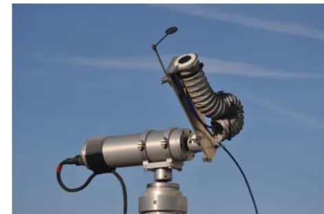
2 The automated halo observation camera HaloCam In order to automatically collect halo observations, the sun-tracking camera system HaloCam was developed at the Me-teorological Institute (MIM) of the Ludwig-Maximilians-Universität (LMU), Munich, and installed on the rooftop platform as shown in Fig. 2. HaloCam consists of a weath-erproof wide-angle camera and is mounted on a sun-tracking system. Using a sun-tracking mount is very suitable for the observation of halo displays and later image processing since it allows the alignment of the center of the camera with the sun. This implies that the recorded halo displays are also cen-tered on the camera pictures. With this setup a small fixed shade is sufficient to protect the camera lens from direct so-lar radiation and to avoid overexposed pixels and stray light. The mount features two stepping motors with gear boxes for adjusting the azimuth and elevation angles of the camera po-sition as described in Seefeldner et al. (2004) with an incre-mental positioning of 2.16 arcmin per step. The positioning of the mount is performed by passively tracking the sun: an algorithm calculates the current position of the sun, which is converted to incremental motor steps and moves the two mo-tors accordingly. The pointing accuracy of the mount can be roughly estimated to about ±0.5◦ (2σ standard deviation), which will be explained in more detail in Sect. 2.3. The cam-era (Mobotix S14D) is a light-weight modular system with an RGB CMOS sensor of 1/200size. Combined with a lens of 22 mm focal length, it provides a horizontal and vertical field of view (FOV) of 90 and 67◦, respectively. Further
specifica-Figure 2.HaloCam: wide-angle camera (Mobotix S14D) with cir-cular shade on a sun-tracking mount. The mount consists of two axes with stepping motors to adjust azimuth and elevation of the camera.
Table 1.HaloCam camera specifications.
Lens
Equivalent 35 mm focal length 22 mm
Nominal focal length 4 mm
Horizontal field of view 90◦
Vertical field of view 67◦
Camera (Mobotix S14D flexmount)
Protection class IP65,−30 to+60◦C
Sensor 1/200CMOS, RGB
progressive scan
Sensor resolution 3 MP
Compression formats JPEG, MxPEG, M-JPEG
tions of the Mobotix S14D camera are listed in Table 1. The camera is operated in an automatic exposure mode and the image region used to determine the optimum exposure time is confined to the region where the 22◦halo occurs. This en-sures that the pixels around the 22◦ halo are not saturated. The camera FOV and the sensor resolution were chosen to optimize the trade-off between a large coverage of the sky with high spatial resolution and low image distortion. Halo-Cam allows for the observation of the 22◦halo, sundogs, and upper/lower tangent arcs or circumscribed halo, which are the most frequent halo displays according to Sassen et al. (2003) and the results of the AKM.
installed in September 2013 on the rooftop platform of MIM (LMU) in Munich, where operational measurements are per-formed by a MIRA-35 cloud radar (Görsdorf et al., 2015), a CHM15kx ceilometer (Wiegner et al., 2014) and a sun pho-tometer, which is part of the AERONET (Aerosol Robotic Network) network (Holben et al., 1998), as well as with the institute’s own sun photometer SSARA (Sun–Sky Automatic Radiometer) (Toledano et al., 2009, 2011). HaloCam obser-vations ideally complement these measurements to retrieve more detailed information about ice crystal properties.
2.1 HaloCam observations – a first statistical evaluation
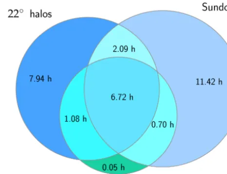
HaloCam has been operated in Munich (Germany) since September 2013, where it provides continuous measure-ments including contributions to the ML-CIRRUS campaign in March and April 2014 (Voigt et al., 2017). It was installed in Cabauw (the Netherlands) only during the ACCEPT cam-paign (Analysis of the Composition of Clouds with Extended Polarization Techniques, Myagkov et al., 2016) in October and November 2014. A first visual evaluation of halo display frequency during ACCEPT (10 October until 14 November 2014) was performed. The results are displayed in Fig. 3 as a Venn diagram (Venn, 1880). The occurrence of each dif-ferent halo type is visualized by a circle. The radius of each circle scales with the total observation time for the respec-tive halo type. Cross sections between the circles indicate in-stances where two or three halo displays were visible at the same time. The observation time is given in hours. The total time of HaloCam observations, which were collected during daytime only, amounts to about 344 h. With about 30 h, halo displays were observed in almost 9 % of the time. The pres-ence of cirrus clouds within the HaloCam field of view was evaluated visually and amounts to about 110 h. Thus, about 27 % of the cirrus clouds produced a visible halo display. The 22◦ halo (complete or partial) occurred in 16.2 %, the sun-dogs in 19 % and the upper tangent arcs in 7.8 % of the time when cirrus clouds were present. Circumscribed halos were not observed during the campaign due to the low solar eleva-tions.
As illustrated in Fig. 3, sundogs were observed more often than 22◦halos, for about 21 vs. 18 h. Thus, sundogs occurred in 70 % and 22◦halos in 60 % of the total halo observation time (30 h). Upper tangent arcs occurred in total for about 9 h (30 %) and were accompanied most of the time by 22◦halos and sundogs. Thus, the majority of the halo displays were produced by oriented ice crystals.
Compared to the findings of Sassen et al. (2003), the rel-ative fraction of 22◦halos is roughly similar with 50 %, but sundogs with 12 % and upper/lower tangent arcs with about 15 % were far less frequent than observed during ACCEPT. The AKM observed the left and right sundogs with a relative frequency of 18 % each, compared to 36 % for the 22◦halos. Although the frequency of simultaneous occurrence of the
Figure 3.Halo display statistics from HaloCam observations dur-ing the ACCEPT campaign 10 October–14 November 2014. The observation times of 22◦halo, sundogs and upper tangent arc are provided in hours and are represented by the radii of the three cir-cles. Cross sections of circles indicate time periods when two or three halo displays were visible simultaneously. The total observa-tion time amounts to 344 h.
(a)
22
◦35
◦46
◦4
4
3
3
2
2
1
1
6
6
5
5
(b)
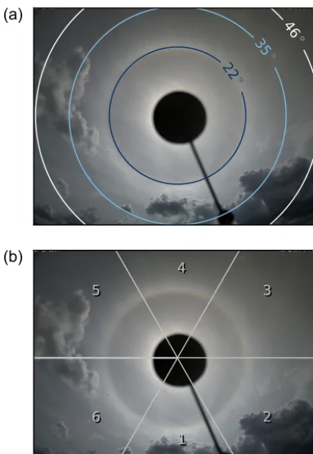
Figure 4. (a)HaloCam image from 12 May 2014, 13:52 UTC, with corresponding scattering angle (ϑ) grid and representative contour lines at 22, 35 and 46◦,(b)shows the relative azimuth (ϕ) grid with numbered labels for the six image segments.
describe how the HaloCam images are processed and which features are extracted for an automated halo detection.
2.2 Camera characterization and calibration
Halo displays are single scattering phenomena and thus are directly linked to the optical properties of the ice crystals producing them. The ice crystal phase function predicts the scattering angle2of the 22◦halo relative to the sun. Thus, the analysis of the HaloCam images can be simplified sig-nificantly by mapping the image pixels to scattering angles. This means the camera has to be calibrated in order to de-termine the parameters for mapping the camera pixels to the real world spherical coordinate system. For this mapping the intrinsic camera parameters have to be determined, which are the focal lengths (fx,fy) and image center coordinates (cx, cy), as well as the distortion coefficients of the camera lens.
Different methods exist for the geometric calibration. Here, we use the method described by Zhang (2000), which is based on Heikkila and Silven (1997), to estimate the in-trinsic camera parameters as well as the radial and tangential
0
50
100
150
200
250
Red
0
50
100
150
200
Brightness [DN]
Green
10
15
20
25
30
35
Scattering angle [o]
0
50
100
150
200
Blue
Figure 5.HaloCam image processing demonstrated for the mea-surements shown in Fig. 4, segment no. 4. The three panels show the brightness distributions (in digital numbers, DN) for the red, green and blue image channel as a function of the scattering angle. The solid line represents the brightness averaged azimuthally over the image segment, whereas the shading indicates the 2σ standard deviation. The vertical lines pinpoint the scattering angles of the 22◦halo minimum (dotted) and maximum (dashed) for the RGB channels.
distortion parameters of the lens. This method requires sev-eral pictures of a planar pattern, for example, a chessboard pattern with known dimensions, taken with different orienta-tions. The calibration method using a chessboard pattern was implemented in OpenCV by Itseez (2015) and is described in detail by Bradski and Kaehler (2008). Using the distortion coefficients and intrinsic parameters, the camera pixels can be undistorted and mapped to the world coordinate system. Thereby a zenith (ϑ) and azimuth angle (ϕ) relative to the image center can be assigned to each pixel. Since the image center is pointing to the center of the sun, the relative zenith angle (ϑ) corresponds to the scattering angle2in this case.
An overlay of the scattering angle grid onto a HaloCam picture is shown in Fig. 4a with representative contour lines atϑ=22, 35 and 46◦. From the scattering angle grid the horizontal and vertical FOV can be calculated to∼93.4 and
∼70.2◦, respectively. HaloCam images are recorded with
a resolution of 1280×960 quadratic pixels, which results in an angular resolution of∼0.07◦for both the horizontal and the vertical direction. Figure 4b shows the relative azimuth angle grid, which is chosen such that the image is separated into six segments. For further analysis and feature extraction, each of these segments is averaged azimuthally.
Table 2.The 22◦ halo features for the example of 12 May 2014 13:52 UTC (as in Fig. 5). The relative zenith angle (which corre-sponds to the scattering angle) is listed for the minimumϑhalo, min and maximumϑhalo, max brightness of the 22◦halo together with the brightness contrast, i.e., the halo ratio (HR) for the red, green and blue image channel.
ϑhalo, min ϑhalo, max HR
Red 18.9◦ 22.0◦ 1.15
Green 19.4◦ 22.0◦ 1.16
Blue 19.8◦ 22.2◦ 1.14
be represented as a data array with 1280×960 elements. As an example the HaloCam image of Fig. 4 is used to demon-strate how the images are processed in case of a 22◦halo.
Figure 5 depicts the brightness distributions of the red, green and blue channel as a function of the scattering angle, aver-aged azimuthally over the uppermost image segment (no. 4 in Fig. 4b). The shaded areas around the lines in Fig. 5 represent twice the standard deviation of the averaged image region.
For analyzing the HaloCam observations several features can be extracted from the brightness distribution across the 22◦halo, which will be explained in the following. The an-gular position of the 22◦halo maximum (ϑhalo, max) is found
by searching for the maximum brightness in the interval (21.0◦, 23.5◦). Then the angular position of the halo mini-mum (ϑhalo, min) is determined by looking for the minimum
brightness in the interval (18.0◦,ϑ
halo, max). Another
impor-tant feature is the brightness contrast of the halo. In previ-ous publications (Gayet et al., 2011; Shcherbakov, 2013; van Diedenhoven, 2014) the so-called “halo ratio” (HR) was in-troduced as a measure for the brightness contrast of the 22◦ and 46◦ halo in the scattering phase function. In analogy, here, the halo ratio is defined as the brightnessI at the scat-tering angle of the halo maximumϑhalo, max divided by the
brightness at the scattering angle of the minimumϑhalo, min:
HR=I (ϑhalo, max)/I (ϑhalo, min). (1)
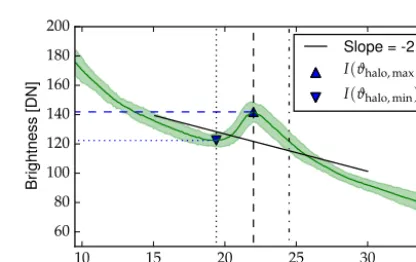
As an example, the values for I (ϑhalo, max) and I (ϑhalo, min) are displayed in Fig. 7 by the blue triangles
pointing up (max) and down (min), respectively. For clear-sky conditions and homogeneous cloud cover, the brightness distribution decreases from the sun towards larger scattering angles, as shown in the example in Figs. 5 and 7. If HR<1 the brightness at the scattering angle of the halo maximum (I (ϑhalo, max)) is smaller than for the minimum (I (ϑhalo, min)),
which is representative for a monotonically decreasing, fea-tureless curve in this scattering angle region. This is the case for clear-sky conditions or homogeneous cloud cover without a halo. For HR=1 the brightnesses at the halo maximum and minimum are the same, causing a slight plateau in the bright-ness distribution. A distinct halo peak occurs for the
condi-Figure 6. Distribution of the scattering angles of the 22◦ halo brightness maximumϑhalo, maxin degrees for 1289 randomly cho-sen and visually classified images using the uppermost image seg-ment (no. 4). The mean value amounts to 21.9◦with a 2σ confi-dence interval of±0.5◦. Note the logarithmic scale of theyaxis.
10 15 20 25 30 35
Scattering angle [o]
60 80 100 120 140 160 180 200
Br
ig
ht
ne
ss
[D
N
]
Slope = -2.5
I(ϑhalo, max) I(ϑhalo, min)
Figure 7.As Fig. 5, showing the first minimum (dotted) and the maximum (dashed) of the 22◦halo for the green channel. In addi-tion,ϑhalo, endis indicated (dash-dotted line), which represents the scattering angle of the same brightness asϑhalo, minand confines the halo peak. In this exampleϑhalo, endis located at about 24.5◦. The corresponding brightness valuesI (ϑhalo, min)andI (ϑhalo, max) used to calculate the HR are marked with blue triangles pointing down (min) and up (max). The regression line of the averaged brightness distribution (solid black), which is evaluated between scattering angles of 15 and 30◦, has a slope of−2.5 for this ex-ample.
tion HR>1. Thus, we assume HR=1 as lower threshold for the visibility of a halo.
For the example of Fig. 5 the 22◦halo features are
com-piled in Table 2, which evaluated for the uppermost im-age segment. The scattering angle of the halo minimum (ϑhalo, min) is smallest for the red channel and largest for the
(Minnaert, 1937; Vollmer, 2006). The differences between scattering angles for the three colors are smaller forϑhalo, max,
with a slightly larger value for the blue channel. The halo ra-tio amounts to about 1.15 averaged over all three channels and is largest for the green and smallest for the blue channel. The angular position of the 22◦ halo brightness peak (ϑhalo, max) can also be used to estimate the positioning
accu-racy of HaloCam relative to the sun. Figure 6 shows a his-togram of ϑhalo, max for 1289 randomly selected HaloCam
pictures showing a 22◦ halo in the uppermost image seg-ment. This segment was chosen since it contains the most pronounced halos. For a faint halo the peak in the bright-ness distribution is rather flat, causing a larger uncertainty in finding the angular position of the peak. The mean value of ϑhalo, max amounts to 21.9◦with a 2σ standard deviation of
0.5◦, which is a rough estimate of HaloCam’s pointing accu-racy. Sinceϑhalo, maxandϑhalo, minare searched for within an
angular interval, the pointing accuracy of±0.5◦is sufficient
to detect the halo.
3 Development of an automated halo detection algorithm
The HaloCam long-term dataset from January 2014 until June 2016 was evaluated by applying a machine learning al-gorithm for the automated detection of halos. The alal-gorithm was trained using features extracted from the HaloCam im-ages. Some of these features (e.g., HR,ϑhalo, max,ϑhalo, min)
were already described in the previous section. As a first im-plementation, the detection algorithm is presented here for the case of the 22◦halo, but it is possible to extend it to other halo types as well.
3.1 Description of the classification algorithm
The detection is performed by a classification algorithm which is trained to predict whether a HaloCam picture be-longs to the class “22◦ halo” or “no 22◦ halo”. For such a binary classification a decision tree can be used to create a model which predicts the class of a data sample. Details on decision trees are explained in Appendix A. One major issue of decision trees is their tendency to overfit by grow-ing arbitrarily complex trees dependgrow-ing on the complexity of the data. In this study we use the random forest classifier as described by Breiman (2001), which improves the issue of overfitting significantly by growing an ensemble of deci-sion trees. A description of the random forest classifier used in this study is provided in Appendix B. In principle, other classification algorithms could be used, like artificial neural networks. The reasons why the random forest classifier was chosen are as follows. Apart from being robust against over-fitting it does not require much preprocessing of the input data like scaling or normalizing. During the training of the individual trees the out-of-bag (OOB) samples (i.e., the
sam-ples which were not in the training subsets) are used as test data, and classification error estimates (e.g., out-of-bag error) can be calculated simultaneously (Breiman, 2001). In con-trast to an artificial neural network, the basic structure and the internal threshold tests of the decision trees are simple to understand and can be explained by boolean logic. Hencefor-ward, the algorithm applied to the classification of 22◦halos will be called HaloForest.
The features used here for the classification are the 22◦halo ratio, the scattering angle position of the halo min-imum and maxmin-imum, and the scattering angle confining the halo peakϑhalo, end, which are shown in Fig. 7 together with
the slope of the regression line in black (solid). The halo peak is confined byϑhalo, end (dash-dotted line), which
rep-resents the scattering angle with the same brightness level asϑhalo, min in the scattering angle interval (ϑhalo, max, 35◦].
This feature is used to ensure that the brightness for angles larger thanϑhalo, maxis decreasing again. The slope of the
re-gression line serves as an estimate for the brightness gradient around the sun. For clear-sky images this gradient is steeper than for overcast cases. As a measure of the separation of color in the halo, the scattering angle difference between the blue and red channel for the halo minimum (1ϑhalo, min) and
maximum (1ϑhalo, max) are calculated, which are defined as 1ϑhalo, max=ϑhalo, max, blue−ϑhalo, max, red,
1ϑhalo, min=ϑhalo, min, blue−ϑhalo, min, red. (2)
Furthermore, the standard deviation of the brightness aver-aged over the image segment is used as a proxy for the inho-mogeneity of the scene. These eight features are calculated for each of the six image segments separately.
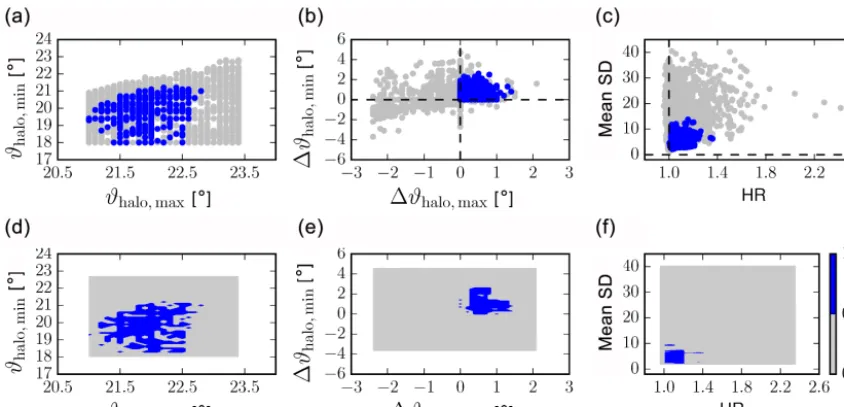
In order to get an impression of typical values of the training features for the two classes, Fig. 8a–c show two-dimensional scatter plots of selected feature pairs for the up-per image segment (no. 4). Features which belong to the class “22◦halo” are displayed in blue, whereas the features of the class “no 22◦ halo” are represented by gray scatter points. Figure 8a shows the distribution of the scattering angle of the halo maximum vs. minimum. The scattering angles of the halo maximum ϑhalo, max are confined to a smaller
in-terval for “22◦halo” compared to “no 22◦halo”. However, the two classes share many data points in this projection, so more features are needed to generate decision boundaries in a higher, here eight-dimensional, space. Figure 8b depicts the scattering angle difference between the blue minus the red channel for the halo maximum (1ϑhalo, max) vs. minimum
(1ϑhalo, max), which is positive for the “22◦halo” class since
the inner edge (smallerϑ) of the 22◦halo is slightly red. The HR, which is shown in Fig. 8c, takes values between 1 and
val-Figure 8. (a–c)Scatter plots of selected pairs of the eight features used for training HaloForest. Training samples with(out) 22◦halos are represented in blue (gray).(d–f)Decision boundaries of the random forest classifier for the respective feature pair. The predicted probability used for separating the classes “22◦halo” (p >0.5) and “no 22◦halo” (p≤0.5) is displayed in blue and gray, respectively.
Table 3.Confusion matrix for HaloForest for the uppermost (no. 4) and lowermost (no. 1) image segments. The label “Predicted” refers to the class which was predicted by HaloForest, whereas “True” la-bels the visually identified class. The true positives (correctly clas-sified “22◦ halo”) are printed in bold font. False positives (“no 22◦ halo” classified as “22◦halo”) and false negatives are listed on the other diagonal. The results are provided with a 2σ standard deviation.
Predicted
Segment 4: 22◦halo no 22◦halo
True 22
◦halo 97.3±1.9 % 0.4±0.3 % no 22◦halo 2.7±0.9 % 99.6±0.2 %
Segment 1: 22◦halo no 22◦halo
True 22
◦
halo 88.5±7.1 % 0.5±0.5 % no 22◦halo 11.5±3.5 % 99.5±0.2 %
ues of the features overlap. The lower panels of Fig. 8d–f display the regions which are detected as “22◦halo” (blue) and “no 22◦halo” (gray) by the trained algorithm.
For each of the six image segments an individual classifier was trained using a dataset of visually classified HaloCam images which were chosen randomly from the dataset. The performance of the classifiers was tested using a random se-lection of 30 % of the dataset which was excluded from train-ing. This procedure was repeated 100 times to get statistically significant results for the performance of the classifier.
Table 3 shows the confusion matrix for the classifier of the segments directly above (no. 4) and below the sun (no. 1) which represent the two extreme cases of the performance
of the six different classifiers: the upper part of the 22◦halo has a higher brightness contrast compared to the lower part which is often obstructed by the horizon. For the training of HaloForest 1289 samples with a 22◦halo and 5181 sam-ples without 22◦halo were used for the uppermost segment (no. 4). The lowermost segment (no. 1) was trained with 296 and 3370 samples of the classes 22◦halo and no 22◦halo,
re-spectively. The lines of the confusion matrix indicate the true class labels of the samples (“22◦halo” and “no 22◦halo”), whereas the columns contain the predicted class labels. The number of true positive and negative (in bold) as well as false positive and negative classifications are evaluated and provided with a 2σ standard deviation. The correct classi-fication of “22◦halo” is maximum for the uppermost image segment (no. 4) with about 98 % and minimum for the lower-most segment with about 89 %. The correct classification of “no 22◦halo” is overall higher than 99 %, so the HaloForest algorithm seems to be able to separate the two classes well. The performance of the other four segments ranges between the results of the upper and lowermost segments.
3.2 Application of the halo detection algorithm
Table 4.Confusion matrix as in Table 3 for 470 randomly selected HaloCam images between January 2014 and June 2016, evaluated for segments 3, 4 and 5. The true positives (correctly classified “22◦halo”) are printed in bold font.
Predicted
22◦halo no 22◦halo
True 22
◦halo 88.8 % 2.8 %
no 22◦halo 11.2 % 97.2 %
the time. As an additional test, the classification accuracy of HaloForest was checked for 470 randomly chosen HaloCam images for the “22◦halo” and “no 22◦halo” class within this long-term observation period in Munich. The confusion ma-trix for this test is provided in Table 4 for the image segments no. 3, 4 and 5 together. More than 88 % of the 22◦halos are
classified correctly and less than 12 % are classified incor-rectly as 22◦halos.
Images were incorrectly classified as 22◦ halo predomi-nantly due to small bright clouds or contrails in a blue sky or structures in overcast conditions which happen to cause a peak in the averaged brightness distribution at a scattering angle of 22◦.
Based on these results we investigated the fraction of cirrus clouds which produced a halo in Munich during this time period. The total frequency of occurrence of cir-rus clouds was determined by independent data of co-located CHM15kx ceilometer observations (Wiegner and Geiß, 2012). To guarantee consistent observational condi-tions, only ceilometer measurements in the absence of low-level clouds were considered. Proprietary software of the ceilometer automatically provides up to three cloud base heights with a temporal resolution of 15 s. The detection is based on the fact that in case of clouds backscatter signals are significantly larger than the background noise.
The sensitivity of the ceilometer is sufficient to even detect clouds near the tropopause during daytime. Since ceilome-ters, however, do not provide depolarization information, the discrimination between water and ice clouds was made by means of the cloud base temperature Tbase. Sassen and
Campbell (2001) state that cirrus cloud base temperatures ranged between−30 and−40◦C during the 10-year obser-vation period at the FARS obserobser-vation site. As a tempera-ture threshold is not an unambiguous criterion for the ex-istence of ice clouds, we have calculated the frequency of occurrence for three different temperatures: −20,−30 and
−40◦C. IfTbase is lower than the given temperature
thresh-old, the cloud is considered a “cirrus cloud”. The tempera-ture profiles were obtained from routine radiosonde ascents of the German Weather Service at Oberschleißheim (WMO station code 10868), which is located about 13 km north of the HaloCam site. During the time period from January 2014 until June 2016 a fraction of 5.6 % cirrus clouds was detected
SZA≥67◦
SZA≥67◦
SZA<67◦
SZA<67◦
4
4
3
3
2
2
1
1
6
6
5
5
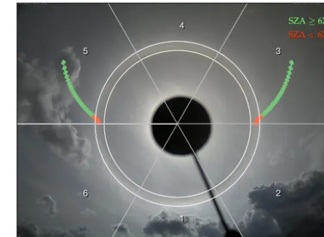
Figure 9.HaloCam image as in Fig. 4b. The red and green squares indicate the minimum scattering angle of the sundogs as a function of the solar zenith angle (SZA). The SZA ranges between 90 and 35◦with 1◦resolution. The mask used to search for the 22◦halo peak is displayed by the two white circles and covers scattering an-gles between 21.0 and 23.5◦. Sundog positions located within this mask might be misclassified as 22◦ halo and are marked as red. These positions correspond with SZAs between 90 and 67◦. For smaller SZAs (higher solar elevations) the sundogs are located out-side the mask and cannot be misclassified as 22◦halo by the algo-rithm.
for a cloud base temperature of Tbase<−20◦C. Towards
lower cloud base temperatures the amount of detected cir-rus clouds decreases to 3.5 % forTbase<−30◦C and 1.9 %
forTbase<−40◦C.
Due to the different pointing directions of the ceilometer (towards zenith) and HaloCam (towards sun), the instruments observe different regions of the sky. This is accounted for by prescreening the data for 1 h time intervals when the ceilome-ter detected a cirrus cloud. The prescreening is subject to data availability for both instruments. The subsequent analysis of cirrus fraction and halo frequency of occurrence is based on the full temporal resolution of 15 and 10 s, respectively. Rel-ative to the amount of detected cirrus clouds about 25 % oc-curred together with a 22◦ halo for the image segments 3, 4 and 5. This fraction does not change much for the dif-ferent cloud base temperatures (26.4 % forTbase<−20◦C
and 24.5 % forTbase<−40◦C) since the fraction of detected
clouds decreases together with the detected halos for lower temperatures. According to the confusion matrix in Table 4, 88.8 % of the detected “22◦ halos” are real halos, while
0.0
0.0
0.1
0.1
0.4
0.4
1.0
1.0
Figure 10.Sky radiance simulations with libRadtran (Mayer and Kylling, 2005) using the DISORT solver for a solar zenith angle of 60◦, a viewing azimuth angle range of 0–160◦and for viewing zenith angles from 10–110◦(i.e., from the zenith to 20◦below the horizon). The simulations were performed for a spectral range of 380–780 nm (5 nm steps), weighted with the spectral sensitivity of the human eye. A homogeneous cirrus cloud layer with optical thickness of 1 was assumed. Solid column ice crystal optical properties of Yang et al. (2013) with an effective radius of 80 µm were used. Aerosol scattering was not considered. The four panels show radiative transfer simulations with different fractions of smooth solid columns ranging from 0 to 100 %, as indicated by the labels. A background of severely roughened solid columns is assumed, with fractions changing from 100 to 0 %, accordingly.
cirrus clouds which produced a 22◦halo within 1 h time in-tervals. The results most likely differ because the observa-tions originate from different locaobserva-tions which might be dom-inated by different mechanisms for cirrus formation. It has to be noted, however, that the evaluation method is very sen-sitive to the sampling strategy of the observations: the frac-tion of halo-producing cirrus clouds increases to more than 50 % if the HaloCam observations are binned to 1 h intervals, which are counted as containing a halo regardless of their du-ration.
For comparison, the fraction of cirrus clouds producing a halo display was evaluated visually for the HaloCam obser-vations during the ACCEPT campaign and amounts to about 27 % including 22◦halos, sundogs and upper/lower tangent
arcs (cf. Sect. 2.1). This value is also lower than the result provided by Sassen et al. (2003) who observed any of the three halo types in about 54 % of the 1 h periods with cirrus. The current version of HaloForest discriminates only be-tween the two classes “22◦ halo” and “no 22◦halo”. Thus, interference with other halo types as sundogs or upper/lower tangent arcs and circumscribed halos might occur at certain solar elevations. The position of sundogs relative to the sun depends on the solar zenith angle (SZA) and can be calcu-lated analytically as described in Wegener (1925), Tricker (1970), Minnaert (1993), and Liou and Yang (2016). The sundogs are located at scattering angles close to the 22◦halo for large SZAs and occur at larger scattering angles for small SZAs, i.e., high solar elevations. Figure 9 shows the same HaloCam image with the azimuth segments as Fig. 4b. In ad-dition, the minimum scattering angle of the sundogs are cal-culated as a function of the SZA and represented by the red and green squares. The SZAs range between 90 and 35◦with a resolution of 1◦. The two white circles centered around the sun at scattering angles of 21.0 and 23.5◦indicate the mask which is used to find the scattering angle of the 22◦ halo peak. For SZA≤67◦ the sundog positions are located out-side this mask and cannot be misclassified as 22◦halo (green
squares). The red squares represent sundog positions which are located within this mask and might therefore be misclas-sified. This is the case for SZAs between 90 and 67◦. To ob-tain an estimate of the fraction of sundogs which are misclas-sified as 22◦halo, 1000 randomly selected HaloCam images were counter-checked visually. This revealed that only six images showing sundogs without 22◦halo in the segments (3–5) were misclassified as 22◦halo, which is<1 %. Upper tangent arcs could be detected by the uppermost image seg-ment (no. 4) and might be misclassified as 22◦halo. For very small SZAs (high solar elevations) the tangent arcs merge to form the circumscribed halo which could be detected in the segments 3 and 5 as well. The same procedure was repeated for these halo types: 1000 randomly selected images were checked for the presence of tangent arcs and circumscribed halos without 22◦halo, yielding 28 images or 2.8 %. How-ever, if only a fragment of a halo is visible in the uppermost segment, it is generally difficult to discriminate between an upper tangent arc or circumscribed halo and a 22◦halo.
The halo classification algorithm was presented for 22◦ ha-los, but it is possible to include training data for other halo types as well. With the current version of HaloForest and the co-located ceilometer observations, the fraction of cirrus clouds producing a halo display was estimated to about 25 % for Munich between January 2014 and September 2016. Ex-tending HaloForest for the detection of other halo types, such as sundogs, the fraction of halo-producing cirrus clouds could easily exceed 25 %. In principle, HaloCam could also be equipped with a wide-angle lens to observe halo displays in a larger region of the sky, however, at the expense of spa-tial resolution.
4 Sensitivity study of the visibility of the 22◦halo and interpretation of halo statistics
22◦ halo. This is important for a more detailed interpreta-tion of the fracinterpreta-tion of halo-producing cirrus clouds and ice crystal roughness.
The effect of varying cloud optical thickness on the visibility of halo displays has been already investigated by Kokhanovsky (2008), Gedzelman and Vollmer (2008), and Gedzelman (2008) using radiative transfer simulations. Kokhanovsky (2008) performed simulations of the bright-ness contrast of the 22◦ halo as a function of the cirrus optical thickness using the radiative transfer model SCIA-TRAN neglecting molecular and aerosol scattering. The re-sults show a linear decrease of the halo contrast with in-creasing optical thickness. Gedzelman (2008) and Gedzel-man and Vollmer (2008) used the model HALOSKY for ra-diative transfer simulations of halos with varying cloud op-tical thickness. HALOSKY considers single scattering by air molecules, aerosol particles and cloud particles assum-ing homogeneous, plane-parallel atmospheric layers. Multi-ple scattering is calculated only within the cloud by a Monte Carlo subroutine. Gedzelman and Vollmer (2008) show re-sults for radiance simulations of the 22◦ halo in the princi-pal plane below and above the sun. They found that the ra-diance at the bottom of the halo reaches a maximum value for smaller COT (≈0.25) than the radiance at the top of the cloud (≈0.63).
In this study, radiative transfer simulations were per-formed using the libRadtran radiative transfer package (Mayer and Kylling, 2005; Emde et al., 2016) and the DIS-ORT (discrete ordinate technique) solver (Stamnes et al., 1988; Buras et al., 2011). LibRadtran allows for an accu-rate simulation of Rayleigh scattering, molecular absorption, aerosols, surface albedo, and water and ice clouds. DIS-ORT is a one-dimensional solver regarding the atmosphere as a number of homogeneous, plane-parallel layers. Radia-tive transfer simulations of a cirrus cloud were performed assuming a homogeneous ice cloud layer with optical thick-ness 1 (at 550 nm) at a height between 10 and 11 km. Fig-ure 10 shows simulations using different fractions of smooth solid columns (0, 10, 40, 100 %) and assuming a background of severely roughened solid columns. All ice crystals have an effective radius of 80 µm. The optical properties were cho-sen from the database by Yang et al. (2013). The sun is lo-cated at a zenith angle of 60◦. Sky radiance was calculated for an angular range between 0 and 160◦ in the azimuth direction and 10–110◦(i.e., from 10◦off-zenith to 20◦ be-low the horizon) in the zenith direction, which corresponds to the view of a wide-angle camera. The simulations were performed for a spectral range of 380–780 nm (5 nm steps), and the results were weighted with the spectral sensitivity of the human eye according to CIE (1986), as implemented in specrend (http://www.fourmilab.ch/documents/specrend/).
Aerosol scattering was not considered and a spectral sur-face albedo of grass was chosen (Feister and Grewe, 1995). For 0 % (first panel of Fig. 10) all ice crystals are rough and thus no 22 or 46◦halo is visible. For a fraction of 10 %
smooth crystals, the 22◦halo starts to form, which is in agree-ment with the findings of van Diedenhoven (2014). The 46◦
halo becomes visible for a fraction of 40 % smooth crys-tals. For 100 % smooth crystals both 22◦and 46◦halo reach a maximum brightness contrast for the respective cirrus opti-cal thickness.
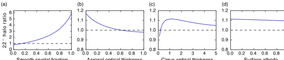
Figure 11 depicts the sensitivity of the halo brightness con-trast, represented by the halo ratio as a function of the smooth ice crystal fraction (a), the aerosol optical thickness (AOT; b), the cirrus optical thickness (c), and the surface albedo (d) for a wavelength of 550 nm. As in Fig. 10 a SZA of 60◦ was chosen and the ice cloud was defined between 10–11 km. The halo ratio was determined in the principal plane above the sun. The dashed lines indicate a halo ratio of 1, which we defined as threshold for the visibility of halo displays. Figure 11a shows clearly that for a smooth crystal fraction of>10 % the halo ratio exceeds 1 and the 22◦halo is
visi-ble. An increasing aerosol optical thickness causes a decrease of the HR, which is displayed in Fig. 11b. For a typical value of AOT=0.2, the HR is reduced by ∼10 % compared to an aerosol free atmosphere. Figure 11c illustrates how the HR is determined by the optical thickness of the cirrus cloud (COT) itself. We observe a maximum value for COT∼1. For a very thin cirrus, Rayleigh and aerosol scattering be-come dominant, resulting in a small HR. The HR approaches its maximum value only when COT is larger than the optical thickness of the background (here Rayleigh and aerosol).
For large COT, multiple scattering reduces the contrast of the halo feature and the HR decreases, similar to the find-ings of Kokhanovsky (2008). However, as Gedzelman and Vollmer (2008) point out, the halo peak might still be visi-ble up to an optical thickness of∼5 due to the pronounced maximum in the scattering phase function.
A higher surface albedo causes longer photon paths through the atmosphere and thus a higher chance of multi-ple scattering (Fig. 11d). Reflected photons therefore cause a higher “background” brightness. It is evident that a brighter background causes a weaker brightness contrast of the halo display. In general, the effect of the surface albedo on the HR is small compared to the effect of AOT or COT. Halo dis-plays are a geometric optics phenomenon, which means that they emerge only when the particle size is much larger than the wavelength (Fraser, 1979; Mishchenko and Macke, 1999; Garrett et al., 2007; Flatau and Draine, 2014), which also depends on the aspect ratio of the crystals (Um and McFar-quhar, 2015). The solar zenith angle affects the halo bright-ness contrast indirectly by increasing the photon path length through the atmosphere for large SZAs and thus increasing the amount of multiple scattering (not shown). This effect is the same for different viewing zenith angles, which explains why the 22◦halo is always brightest at the top (directly above the sun) and faintest below the sun.
0.0 0.2 0.4 0.6 0.8 1.0
Smooth crystal fraction
0
1 2 3 4 5 6
2
2
◦ h
a
lo
r
a
ti
o
(a)
0.0 0.2 0.4 0.6 0.8 1.0
Aerosol optical thickness
0.8 0.9 1.0 1.1 1.2
(b)
0 1 2 3 4 5
Cirrus optical thickness
0.8 0.9 1.0 1.1 1.2
(c)
0.0 0.2 0.4 0.6 0.8 1.0
Surface albedo
0.8 0.9 1.0 1.1 1.2
(d)
Figure 11.Sensitivity studies of the 22◦halo ratio at 550 nm (as defined in Eq. 1) as a function of smooth crystal fraction, aerosol optical thickness (AOT), cirrus optical thickness (COT) and surface albedo (from left to right). The radiative transfer simulations were performed with libRadtran assuming an ice cloud between 10 and 11 km using ice crystal optical properties as in Fig. 10 for a solar zenith angle of 60◦. The dashed line indicates HR=1, which marks the threshold for the visibility of a halo display. The default parameters, i.e., if not varied, are 20 % smooth solid columns, AOT=0.2, COT=1.0 and albedo=0.0.
which were visible from the ground, produced a 22◦halo. It can be argued that these cirrus clouds contained a certain amount of smooth, hexagonal ice crystals. By analyzing ice crystal single scattering properties, van Diedenhoven (2014) showed that a minimum fraction of 10 % smooth hexago-nal ice crystal columns is sufficient to produce a 22◦halo. With about 40 %, the minimum fraction of smooth crystals is much larger in the case of ice crystal plates for a visible halo. Thus, if the exact ice crystal habits of the cirrus cloud are unknown, which is typically the case, the minimum amount of smooth ice crystals probably lies in a range of 10 to 40 %. This implies that even for a large fraction of irregular or small ice crystals a halo might still be visible. A larger fraction of smooth ice crystals, however, could well be possible for halos with larger HR, i.e., increased brightness contrast. Multiple scattering of the cirrus cloud or atmosphere was not consid-ered by van Diedenhoven (2014). This study revealed that during the∼2.5 years of HaloCam observations in Munich about 75 % of the cirrus clouds did not produce a 22◦halo. For favorable atmospheric conditions, i.e., COT∼1 and neg-ligible aerosol scattering, the maximum fraction of rough ice crystals ranges between 60 and 90 %. Thus, it is possi-ble that the majority of cirrus clouds during the observation period in Munich contain a large fraction of rough ice crys-tals. This would support the hypothesis of Knap et al. (2005), Baran and Labonnote (2006), and Baran et al. (2015), who found that on average rough ice crystals better reproduce re-mote sensing radiance measurements than assuming crystals with smooth surface. However, if multiple scattering by cir-rus clouds or aerosol is accounted for, the minimum fraction of smooth crystals could be much larger in the case of halo-producing cirrus clouds. The actual fraction of smooth ice crystals for cirrus clouds with visible halo display must be analyzed in detail and will be addressed in future work. This requires HaloCam observations to be complemented by ra-diative transfer simulations and additional measurements of aerosol and cirrus optical thickness. These additional mea-surements can be provided by radar, lidar and sun
photome-ter measurements available at the observation site at MIM, LMU, in Munich. Surface albedo measurements can be ob-tained from satellite data products.
5 Summary and conclusions
In this paper we present HaloCam, a novel sun-tracking cam-era system for the automated observation of halo displays. The camera has a field of view of 90◦in the horizontal and 67◦in the vertical direction and a resolution of 1280×960 quadratic pixels which yields an angular resolution of 0.07◦. The camera system records images in RGB color space and JPEG compression every 10 s. It automatically tracks the sun so that the halo displays stay centered relative to the camera. HaloCam observations can contribute to a better understand-ing of ice crystal shape, surface roughness and orientation by long-term observations of halo displays. Different halo dis-plays are caused by different ice crystal shapes and orienta-tions. The most frequent halo displays are formed by either randomly oriented or oriented plates and columns and there-fore contain the most important information about ice crys-tal properties. Therefore, the camera setup was optimized for observing 22◦halos, sundogs, and upper/lower tangent arcs or circumscribed halos with high spatial and temporal reso-lution without loosing relevant information.
visible. It should be highlighted that the evaluation method is very sensitive to the sampling method and the temporal resolution of the observations.
For evaluating the long-term HaloCam observations in Munich, an automated halo detection algorithm, called Halo-Forest, was developed. HaloForest is presented here for the detection of 22◦halos, but it can be extended for the detec-tion of other halo types such as sundogs and upper/lower tan-gent arcs. The algorithm is based on a random forest clas-sifier and was trained and tested against visually evaluated observations. With more than 88 % of the test samples cor-rectly classified as “22◦halos” and more than 97 % correctly classified as “no 22◦halo”, HaloForest is able to separate the two classes well. Applied to the more than 2.5 years of data, HaloForest detected 22◦halos about 2 % of the total obser-vation time during daylight.
A first estimate of ice crystal roughness was performed by evaluating the frequency of cirrus clouds that were ac-companied by halo displays. For the long-term halo observa-tions in Munich, co-located ceilometer measurements were used to evaluate the fraction of cirrus clouds. About 25 % of the detected cirrus clouds in Munich occurred together with a 22◦halo. Extending HaloForest for more halo types (e.g., sundogs) would increase the fraction of halo-producing cir-rus clouds above 25 %.
These results imply that the majority of cirrus clouds which did not produce a visible halo, very likely, contained primarily rough ice crystals and 25 % (or 27 % for ACCEPT) of the clouds contained at least a certain fraction of smooth, hexagonal ice crystals. Based on the study by van Dieden-hoven (2014) a minimum fraction of smooth crystals of 10 % in case of columns or 40 % in case of plates can be estimated for the halo-producing cirrus clouds if multiple scattering and scattering by aerosol is neglected. These assumptions allow determining a minimum fraction of smooth crystals in halo-producing cirrus clouds. If multiple scattering by cloud and aerosol is accounted for, the required fraction of smooth ice crystals could be significantly larger than 40 %. To further constrain the fraction of rough ice crystals, more detailed quantitative studies are needed, which will be addressed in future work. This analysis requires radiative transfer simu-lations and additional constraints which can be provided by radar, lidar and sun photometer measurements available at the observation site at LMU in Munich.
This study highlights the potential and feasibility of a com-pletely automated method to collect and evaluate halo obser-vations. These long-term observations allow estimating the average fraction of rough ice crystals in cirrus clouds. Quan-titative evaluation of halo radiance distributions can con-tribute to systematically investigate ice crystal surface rough-ness, shape and orientation in cirrus clouds. Implemented on different sites, HaloCam in combination with the HaloFor-est detection algorithm can provide a consistent dataset for climatological studies.
Data availability. The radiosonde data are available via the web-site of the University of Wyoming, College of Engineering, Depart-ment of Atmospheric Science, at http://weather.uwyo.edu/upperair/ sounding.html. Due to the large file size, the HaloCam images and the ceilometer data from the measurement site at the Meteorologi-cal Institute (LMU) in Munich from January 2014 until June 2016 will be provided upon request. A sample HaloCam image is pro-vided in the Supplement, which is the underlying source of the data of Table 2 and Figs. 4, 5, 7 and 9.
Appendix A: Decision trees
The subsequent sections provide more details on decision trees and the random forest classifier presented in Sect. 3.
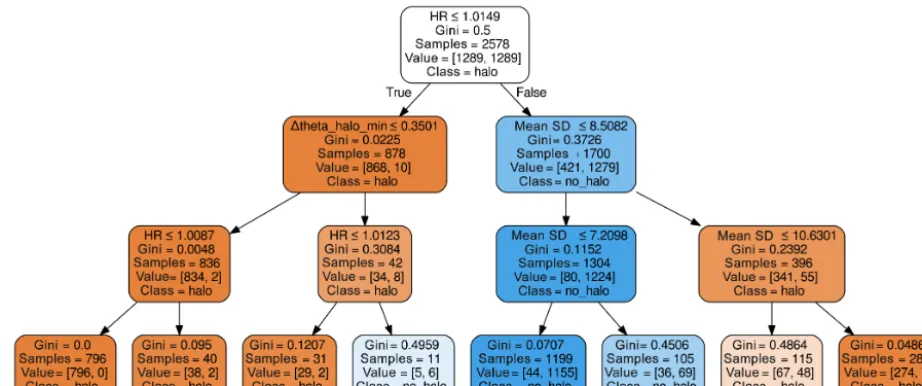
The following description is based on Alpaydin (2010) and Raschka (2015). Decision trees start with a root node followed by internal decision nodes, branches and terminal nodes, called leaves. A typical example of a single decision tree, as used for HaloForest, is shown in Fig. A1. For a bet-ter visualization, the tree is grown using only three of the eight features and is pruned to a depth of three layers. The explanation provided here focuses on the structure of tree rather than the exact numbers of the threshold tests which differ from the ones used by HaloForest. The halo ratio (HR), the mean standard deviation and1ϑhalo, minare used as
fea-tures in this case, which are displayed in the first line of each node box with the respective threshold test. At each deci-sion node a threshold test is applied to one element of the n-dimensional feature vector (here,n=3) which best splits the set of samples. The metric to determine the best split in this study is the Gini impurity index, which is defined by Raschka (2015) as
IG(t )=1− c X
i=1
p(i|t )2, (A1)
withcbeing the number of classes andp(i|t )the fraction of samples which belongs to classiat nodet. The Gini index takes a minimum value for the maximum information gain (all the samples at nodetbelong to one class), and the index is maximum for a uniform distribution. The discrete result (here, true or false) of the threshold test decides which of the following branches is chosen. The node boxes are connected by arrows representing the branches of the tree. They are colored depending on the dominating class in the samples, which is noted at the bottom of each box: red for “22◦halo”
and blue for “no 22◦halo”. The more transparent the color
the higher the impurity of the classes and the larger the Gini impurity index. This splitting process is repeated recursively at each child node until a leaf node is reached. A leaf node is hit when all the samples in the subset belong to the same class or when splitting does not add more information. By repeat-ing this recursive decision process, then-dimensional feature space is subdivided into the predefined classes on a path fol-lowing from the root down. Figure 8 shows examples of the resulting decision boundaries as two-dimensional projections for a selection of feature pairs. The decision tree is trained us-ing a set of labeled trainus-ing samples. Durus-ing trainus-ing the tree grows by adding branches and leaves depending on the com-plexity of the data, which can lead to overfitting. By growing an ensemble of decision trees, this issue can be improved, which is the idea of random forest classifiers.
Appendix B: Random forest classifier implementation In this study we use the random forest classifier, which is de-scribed by Breiman (2001) and implemented in the python module scikit-learn (Pedregosa et al., 2011, version 0.18.1). The trees are trained by applying the bootstrap aggregation (bagging) method (Breiman, 1996), i.e., by using a subset of the training samples which is chosen randomly with replace-ment and has the same size as the original input samples. This implementation predicts the class of a sample by averaging the probabilistic prediction of all individual decision trees in-stead of using the majority vote among the trees. The func-tion call allows the definifunc-tion of a number of parameters: the number of trees is set to 100 and a maximum number of three features (log2(n)withnfeatures) is considered for searching the best split. These parameters are chosen to minimize the out-of-bag (OOB) error, as shown in Fig. B1.
Figure A1.Example for a decision tree for a selection of three HaloCam image features confined to a maximum depth of three layers. The two classes, “halo” and “no halo”, are depicted by red and blue color. The transparency of the color represents the impurity of the class.
50 100 150 200 250 300
n_estimators
0.7 0.8 0.9 1.0 1.1 1.2 1.3 1.4
OOB error rate [%]
Max_features = none Max_features = 'log2' Max_features = 'sqrt'
Competing interests. The authors declare that they have no conflict of interest.
Acknowledgements. The radiosonde data were downloaded from http://weather.uwyo.edu/upperair/sounding.html from the University of Wyoming, College of Engineering, Department of Atmospheric Science. The halo observations during the ACCEPT campaign research received funding from the European Union Sev-enth Framework Program (FP7/2007-2013) under grant agreement no 262254. We thank Markus Garhammer (LMU, Munich) and Marc Allaart (KNMI, the Netherlands) for their support during the campaign.
Edited by: Murray Hamilton
Reviewed by: Bastiaan van Diedenhoven and two anonymous referees
References
Alpaydin, E.: Introduction to Machine Learning, Adaptive Compu-tation and Machine Learning, 2nd edn., MIT Press, Cambridge, 2010.
Baran, A. J. and Labonnote, L. C.: On the reflection and polarisation properties of ice cloud , J. Quant. Spectrosc. Ra., 100, 41–54, https://doi.org/10.1016/j.jqsrt.2005.11.062, 2006.
Baran, A. J., Furtado, K., Labonnote, L.-C., Havemann, S., The-len, J.-C., and Marenco, F.: On the relationship between the scat-tering phase function of cirrus and the atmospheric state, At-mos. Chem. Phys., 15, 1105–1127, https://doi.org/10.5194/acp-15-1105-2015, 2015.
Bradski, D. G. R. and Kaehler, A.: Learning Opencv, 1st edn., O’Reilly Media, Inc., Sebastopol, 2008.
Breiman, L.: Bagging Predictors, Mach. Learn., 24, 123–140, https://doi.org/10.1023/A:1018054314350, 1996.
Breiman, L.: Random forests, Mach. Learn., 45, 5–32, https://doi.org/10.1023/A:1010933404324, 2001.
Buras, R., Dowling, T., and Emde, C.: New secondary-scattering correction in DISORT with increased efficiency for forward scat-tering, J. Quant. Spectrosc. Ra., 112, 2028–2034, 2011. CIE: Standard on Colorimetric Observers, Commission
Interna-tionale de l’Eclairage CIE, 1986.
Emde, C., Buras-Schnell, R., Kylling, A., Mayer, B., Gasteiger, J., Hamann, U., Kylling, J., Richter, B., Pause, C., Dowling, T., and Bugliaro, L.: The libRadtran software package for radia-tive transfer calculations (version 2.0.1), Geosci. Model Dev., 9, 1647–1672, https://doi.org/10.5194/gmd-9-1647-2016, 2016. Feister, U. and Grewe, R.: Spectral albedo measurements in the
UV and visible region over different types of surfaces, Pho-tochem. Photobiol., 62, 736–744, https://doi.org/10.1111/j.1751-1097.1995.tb08723.x, 1995.
Flatau, P. J. and Draine, B. T.: Light scattering by hexagonal columns in the discrete dipole approximation, Opt. Express, 22, 21834–21846, https://doi.org/10.1364/OE.22.021834, 2014. Fraser, A. B.: What size of ice crystals causes
the halos?, J. Opt. Soc. Am., 69, 1112–1118, https://doi.org/10.1364/JOSA.69.001112, 1979.
Garrett, T. J., Kimball, M. B., Mace, G. G., and Baumgardner, D. G.: Observing cirrus halos to constrain in-situ measurements of ice crystal size, Atmos. Chem. Phys. Discuss., 7, 1295-1325, https://doi.org/10.5194/acpd-7-1295-2007, 2007.
Gayet, J.-F., Mioche, G., Shcherbakov, V., Gourbeyre, C., Busen, R., and Minikin, A.: Optical properties of pristine ice crystals in mid-latitude cirrus clouds: a case study during CIRCLE-2 experiment, Atmos. Chem. Phys., 11, 2537–2544, https://doi.org/10.5194/acp-11-2537-2011, 2011.
Gedzelman, S. D.: Simulating halos and coronas in their atmospheric environment, Appl. Optics, 47, H157–H166, https://doi.org/10.1364/AO.47.00H157, 2008.
Gedzelman, S. D. and Vollmer, M.: Atmospheric optical phenom-ena and radiative transfer, B. Am. Meteorol. Soc., 89, 471–485, https://doi.org/10.1175/BAMS-89-4-471, 2008.
Görsdorf, U., Lehmann, V., Bauer-Pfundstein, M., Peters, G., Vavriv, D., Vinogradov, V., and Volkov, V.: A 35-GHz polari-metric doppler radar for long-term observations of cloud pa-rameters – description of system and data processing, J. Atmos. Ocean. Tech., 32, 675–690, https://doi.org/10.1175/JTECH-D-14-00066.1, 2015.
Greenler, R.: Rainbows, halos and glories, Cambridge University Press, Cambridge, 1980.
Heikkila, J. and Silven, O.: A four-step camera calibration proce-dure with implicit image correction, in: Proceedings of IEEE Computer Society Conference on Computer Vision and Pattern Recognition, 17–19 June 1997, San Juan, Puerto Rico, USA, 1106–1112, https://doi.org/10.1109/CVPR.1997.609468, 1997. Holben, B., Eck, T., Slutsker, I., Tanré, D., Buis, J., Setzer, A.,
Ver-mote, E., Reagan, J., Kaufman, Y., Nakajima, T., Lavenu, F., Jankowiak, I., and Smirnov, A.: AERONET – a federated in-strument network and data archive for aerosol characterization, Remote Sens. Environ., 66, 1–16, https://doi.org/10.1016/S0034-4257(98)00031-5, 1998.
Itseez: Open Source Computer Vision Library, available at: https: //github.com/itseez/opencv (10 July 2017), 2015.
Knap, W. H., Labonnote, L. C., Brogniez, G., and Stammes, P.: Modeling total and polarized reflectances of ice clouds: evalu-ation by means of POLDER and ATSR-2 measurements, Appl. Optics, 44, 4060–4073, https://doi.org/10.1364/AO.44.004060, 2005.
Kokhanovsky, A.: The contrast and brightness of ha-los in crystalline clouds, Atmos. Res., 89, 110–112, https://doi.org/10.1016/j.atmosres.2007.12.006, 2008.
Liou, K. and Yang, P.: Light Scattering by Ice Crystals: Fundamen-tals and Applications, Cambridge University Press, Cambridge, 2016.
Lynch, D. K. and Schwartz, P.: Intensity profile of the 22◦ halo, J. Opt. Soc. Am. A, 2, 584–589, https://doi.org/10.1364/JOSAA.2.000584, 1985.
Mayer, B. and Kylling, A.: Technical note: The libRadtran soft-ware package for radiative transfer calculations - description and examples of use, Atmos. Chem. Phys., 5, 1855–1877, https://doi.org/10.5194/acp-5-1855-2005, 2005.
Minnaert, M.: De natuurkunde van ’t vrije veld. Deel I. Licht en kleur in het landschap, W. J. Thieme, Zutphen, 1937.
Mishchenko, M. and Macke, A.: How big should hexagonal ice crystals be to produce halos?, Appl. Optics, 38, 1626–1629, https://doi.org/10.1364/AO.38.001626, 1999.
Myagkov, A., Seifert, P., Wandinger, U., Bühl, J., and Engelmann, R.: Relationship between temperature and apparent shape of pris-tine ice crystals derived from polarimetric cloud radar obser-vations during the ACCEPT campaign, Atmos. Meas. Tech., 9, 3739–3754, https://doi.org/10.5194/amt-9-3739-2016, 2016. Pedregosa, F., Varoquaux, G., Gramfort, A., Michel, V., Thirion, B.,
Grisel, O., Blondel, M., Prettenhofer, P., Weiss, R., Dubourg, V., Vanderplas, J., Passos, A., Cournapeau, D., Brucher, M., Per-rot, M., and Duchesnay, E.: Scikit-learn: machine learning in Python, J. Mach. Learn. Res., 12, 2825–2830, 2011.
Pekkola, M.: Finnish Halo Observing Network: search for rare halo phenomena, Appl. Optics, 30, 3542–3544, https://doi.org/10.1364/AO.30.003542, 1991.
Pernter, J. M. and Exner, F.: Meteorologische Optik, W. Braumüller, Wien, 1910.
Raschka, S.: Python Machine Learning, Community experience dis-tilled, Packt Publishing, Birmingham, 2015.
Sassen, K. and Campbell, J. R.: A midlatitude cirrus cloud climatology from the facility for atmospheric remote sens-ing. Part I: Macrophysical and synoptic properties, J. Atmos. Sci., 58, 481–496, https://doi.org/10.1175/1520-0469(2001)058<0481:AMCCCF>2.0.CO;2, 2001.
Sassen, K., Zhu, J., and Benson, S.: Midlatitude cirrus cloud climatology from the facility for atmospheric remote sensing. IV. Optical displays, Appl. Optics, 42, 332–341, https://doi.org/10.1364/AO.42.000332, 2003.
Seefeldner, M., Oppenrieder, A., Rabus, D., Reuder, J., Schreier, M., Hoeppe, P., and Koepke, P.: A two-axis tracking system with datalogger, J. Atmos. Ocean. Tech., 21, 975–979, https://doi.org/10.1175/1520-0426(2004)021<0975:ATTSWD>2.0.CO;2, 2004.
Shcherbakov, V.: Why the 46◦ halo is seen far less often than the 22◦ halo?, J. Quant. Spectrosc. Ra., 124, 37–44, https://doi.org/10.1016/j.jqsrt.2013.03.002, 2013.
Stamnes, K., Tsay, S., Wiscombe, W., and Jayaweera, K.: A nu-merically stable algorithm for discrete-ordinate-method radiative transfer in multiple scattering and emitting layered media, Appl. Optics, 27, 2502–2509, https://doi.org/10.1364/AO.27.002502, 1988.
Tape, W.: Atmospheric halos, Antarctic Research Series, American Geophysical Union, Washington DC, 1994.
Tape, W. and Moilanen, J.: Atmospheric Halos and the Search for Angle X, American Geophysical Union, Washington DC, 2006. Toledano, C., Wiegner, M., Garhammer, M., Seefeldner, M.,
Gasteiger, J., Müller, D., and Koepke, P.: Spectral aerosol op-tical depth characterization of desert dust during SAMUM 2006, Tellus B, 61, 216–228, https://doi.org/10.1111/j.1600-0889.2008.00382.x, 2009.
Toledano, C., Wiegner, M., Groß, S., Freudenthaler, V., Gasteiger, J., Müller, D., Müller, T., Schladitz, a., Weinzierl, B., Torres, B., and O’Neill, N. T.: Optical properties of aerosol mixtures derived from sun-sky radiometry during SAMUM-2, Tellus B, 63, 635–648, https://doi.org/10.1111/j.1600-0889.2011.00573.x, 2011.
Tricker, R. A. R.: Introduction to Meteorological Optics, Elsevier, New York, 1970.
Um, J. and McFarquhar, G. M.: Formation of atmospheric ha-los and applicability of geometric optics for calculating single-scattering properties of hexagonal ice crystals: Impacts of aspect ratio and ice crystal size, J. Quant. Spectrosc. Ra., 165, 134–152, https://doi.org/10.1016/j.jqsrt.2015.07.001, 2015.
van Diedenhoven, B.: The prevalence of the 22◦ halo in cirrus clouds, J. Quant. Spectrosc. Ra., 146, 475–479, https://doi.org/10.1016/j.jqsrt.2014.01.012, 2014.
Venn, J.: On the employment of geometrical diagrams for the sensi-ble representations of logical propositions, P. Camb. Philos. Soc., 4, 47–59, 1880.
Verschure, P.-P. H.: Thirty years of observing and document-ing sky optical phenomena, Appl. Optics, 37, 1585–1588, https://doi.org/10.1364/AO.37.001585, 1998.
Voigt, C., Schumann, U., Minikin, A., Abdelmonem, A., Af-chine, A., Borrmann, S., Boettcher, M., Buchholz, B., Bugliaro, L., Costa, A., Curtius, J., Dollner, M., Dörnbrack, A., Dreiling, V., Ebert, V., Ehrlich, A., Fix, A., Forster, L., Frank, F., Fütterer, D., Giez, A., Graf, K., Grooß, J.-U., Groß, S., Heimerl, K., Heinold, B., Hüneke, T., Järvinen, E., Jurkat, T., Kaufmann, S., Kenntner, M., Klingebiel, M., Kli-mach, T., Kohl, R., Krämer, M., Krisna, T. C., Luebke, A., Mayer, B., Mertes, S., Molleker, S., Petzold, A., Pfeilsticker, K., Port, M., Rapp, M., Reutter, P., Rolf, C., Rose, D., Sauer, D., Schäfler, A., Schlage, R., Schnaiter, M., Schneider, J., Spel-ten, N., Spichtinger, P., Stock, P., Walser, A., Weigel, R., Weinzierl, B., Wendisch, M., Werner, F., Wernli, H., Wirth, M., Zahn, A., Ziereis, H., and Zöger, M.: ML-CIRRUS: the air-borne experiment on natural cirrus and contrail cirrus with the high-altitude long-range research aircraft HALO, B. Am. Me-teorol. Soc., 98, 271–288, https://doi.org/10.1175/BAMS-D-15-00213.1, 2017.
Vollmer, M.: Lichtspiele in der Luft, 1st edn., Spektrum Akademis-cher Verlag, München, 2006.
Wegener, A.: Theorie der Haupthalos, Aus dem Archiv der Deutschen Seewarte und des Marineobservatoriums, Hamburg, 43, 1925.
Wendisch, M., Yang, P., and Pilewskie, P.: Effects of ice crystal habit on thermal infrared radiative properties and forcing of cirrus, J. Geophys. Res., 112, D08201, https://doi.org/10.1029/2006JD007899, 2007.
Wiegner, M. and Geiß, A.: Aerosol profiling with the Jenop-tik ceilometer CHM15kx, Atmos. Meas. Tech., 5, 1953–1964, https://doi.org/10.5194/amt-5-1953-2012, 2012.
Wiegner, M., Madonna, F., Binietoglou, I., Forkel, R., Gasteiger, J., Geiß, A., Pappalardo, G., Schäfer, K., and Thomas, W.: What is the benefit of ceilometers for aerosol remote sensing? An answer from EARLINET, Atmos. Meas. Tech., 7, 1979–1997, https://doi.org/10.5194/amt-7-1979-2014, 2014.
Wylie, D., Menzel, W., Woolf, H., and Strabala, K.: Four years of global cirrus cloud statistics using HIRS, J. Climate, 7, 1972– 1986, 1994.
Yang, P., Bi, L., Baum, B. A., Liou, K.-N., Kattawar, G. W., Mishchenko, M. I., and Cole, B.: Spectrally consistent scatter-ing, absorption, and polarization properties of atmospheric ice crystals at wavelengths from 0.2 to 100 µm, J. Atmos. Sci., 70, 330–347, https://doi.org/10.1175/JAS-D-12-039.1, 2013. Yang, P., Liou, K.-N., Bi, L., Liu, C., Yi, B., and Baum, B. A.:
sensing, and radiation parameterization, Adv. Atmos. Sci., 32, 32–63, https://doi.org/10.1007/s00376-014-0011-z, 2015. Yi, B., Yang, P., Baum, B. A., L’Ecuyer, T., Oreopoulos, L.,
Mlawer, E. J., Heymsfield, A. J., and Liou, K.-N.: Influence of ice particle surface roughening on the global cloud radiative ef-fect, J. Atmos. Sci., 70, 2794–2807, https://doi.org/10.1175/JAS-D-13-020.1, 2013.