www.atmos-meas-tech.net/9/4803/2016/ doi:10.5194/amt-9-4803-2016
© Author(s) 2016. CC Attribution 3.0 License.
Absolute calibration of the colour index and O
4
absorption derived
from Multi AXis (MAX-)DOAS measurements and their application
to a standardised cloud classification algorithm
Thomas Wagner, Steffen Beirle, Julia Remmers, Reza Shaiganfar, and Yang Wang Max-Planck-Institute for Chemistry, Mainz, Germany
Correspondence to:Thomas Wagner ([email protected])
Received: 27 April 2016 – Published in Atmos. Meas. Tech. Discuss.: 30 May 2016
Revised: 6 September 2016 – Accepted: 15 September 2016 – Published: 28 September 2016
Abstract. A method is developed for the calibration of the colour index (CI) and the O4 absorption derived from
dif-ferential optical absorption spectroscopy (DOAS) measure-ments of scattered sunlight. The method is based on the comparison of measurements and radiative transfer simula-tions for well-defined atmospheric condisimula-tions and viewing geometries. Calibrated measurements of the CI and the O4
absorption are important for the detection and classification of clouds from MAX-DOAS observations. Such information is needed for the identification and correction of the cloud influence on Multi AXis (MAX-)DOAS profile inversion re-sults, but might be also be of interest on their own, e.g. for meteorological applications. The calibration algorithm was successfully applied to measurements at two locations: Cabauw in the Netherlands and Wuxi in China. We used CI and O4observations calibrated by the new method as input
for our recently developed cloud classification scheme and also adapted the corresponding threshold values accordingly. For the observations at Cabauw, good agreement is found with the results of the original algorithm. Together with the calibration procedure of the CI and O4absorption, the cloud
classification scheme, which has been tuned to specific lo-cations/conditions so far, can now be applied consistently to MAX-DOAS measurements at different locations. In addi-tion to the new threshold values, further improvements were introduced to the cloud classification algorithm, namely a better description of the SZA (solar zenith angle) dependence of the threshold values and a new set of wavelengths for the determination of the CI. We also indicate specific areas for future research to further improve the cloud classification scheme.
1 Introduction
Multi AXis differential optical absorption spectroscopy (MAX-DOAS) measurements are a widely used remote sens-ing technique for the measurement of atmospheric trace gases and aerosols (e.g. Hönninger and Platt, 2002; Wittrock et al., 2004; Hönninger et al., 2004; Heckel et al., 2005; Frieß et al., 2006; Irie et al., 2008; Clémer et al., 2010; Li et al., 2010; Wagner et al., 2011; Ma et al., 2013; Hen-drick et al., 2014; Wang et al., 2014, 2015; Vlemmix et al., 2015). MAX-DOAS measurements can be strongly affected by clouds (Wagner et al., 2004, 2011, 2014; Gielen et al., 2014; Wang et al., 2015). Thus cloud-contaminated measure-ments have to be flagged, excluded from further processing or corrected for the effects of clouds. Different algorithms for the identification and classification of clouds based on MAX-DOAS measurements have recently been developed. They are based on several quantities derived from the mea-sured spectra (Wagner et al., 2014; Gielen et al., 2014; Wang et al., 2015). These quantities include the following.
a. A so-called colour index (CI, see e.g. Sarkissian et al., 1991, 1994), which is defined as the intensity ratio for two selected wavelengths. In this study we define the CI as a ratio of the intensity at the shorter wavelength to the intensity at the longer wavelength:
CI=Ishort
Ilong
. (1)
are not radiometrically calibrated. Thus we use the term “radiance” here in a broader sense for the measured sig-nal as well, e.g. expressed as counts per second. c. The absorption of the oxygen dimer O4(Greenblatt et
al., 1990).
d. The strength of the so-called Ring effect (the filling-in of solar Fraunhofer lines by rotational Raman scatter-ing, see Grainger and Rscatter-ing, 1962; Wagner et al., 2014). It was shown by Gielen et al. (2014) and Wagner et al. (2014) that the CI is very sensitive to the presence of clouds. It is thus well suited for their detection, especially because for zenith observations, clouds always lead to a de-crease of the CI compared to clear-sky conditions (if the CI is defined with the intensity at the shorter wavelength divided by the intensity at the longer wavelength). In contrast, the other quantities mentioned above can be both increased or decreased in the presence of clouds depending on the cloud properties, wavelength and viewing geometry. Because of the unique dependence of the CI on the occurrence of clouds, the CI is usually used as the primary quantity for the detection of clouds. From the other quantities, especially from the ra-diance and the absorption of the oxygen dimer O4,
impor-tant additional information on cloud properties can be de-rived (e.g. the presence of optically thick clouds or fog, see Wagner et al., 2014; Gielen et al., 2014; Wang et al., 2015). Since Ring effect measurements do not provide significant extra information, and because the quantitative analysis of the Ring effect is rather complicated, the Ring effect is not further considered here.
The identification and classification of clouds is usually based on the comparison of the measured quantities with their thresholds. These threshold values can e.g. be derived from measurements on clear days. Another, more universal, method is the determination of the threshold values from ra-diative transfer simulations. However, since MAX-DOAS in-struments are usually not radiometrically calibrated, a direct quantitative comparison of measured and simulated quanti-ties is not possible, which hampers the direct application of threshold values derived from radiative transfer simulations. To overcome this limitation, in this study we develop calibra-tion procedures for the CI and the O4 absorption and apply
them to MAX-DOAS observations.
The proposed CI calibration comprises the determination of a proportionality constant, which converts the measured values into well-defined quantities (i.e. radiance ratios for the selected wavelengths). Similar suggestions for the calibration of the CI were already presented by Gielen et al. (2014) and Wagner et al. (2014).
For the O4 measurements, the calibration comprises the
determination and correction of an additional offset (the O4
absorption of the Fraunhofer reference spectrum, FRS) like in Wagner et al. (2014). Already in Wagner et al. (2014) the measured CI and O4were calibrated based on selected
clear-sky measurements. In contrast, here we develop standardised calibration algorithms for CI and the O4 absorption, which
can be applied to other MAX-DOAS measurements in a con-sistent way.
Update of the cloud classification scheme
After applying the new calibration algorithms to the mea-surements the calibrated CI and the O4 absorption differ
slightly from the calibrated values of the original classifica-tion scheme. Thus the threshold values of the cloud classifi-cation scheme have to be adapted accordingly. In addition to these changes, further improvements to the original classifi-cation scheme (Wagner et al., 2014) are introduced.
a. The determination of the threshold values is based on well-defined atmospheric scenarios.
b. The new thresholds better account for solar zenith angle (SZA) dependencies.
c. A new set of wavelengths is used for the CI: the old wavelength pair (320 nm/440 nm, see Wagner et al., 2014) is replaced by 330 nm/390 nm. The new wave-length pair has several advantages: the new shorter wavelength (330nm) is less affected by the atmospheric ozone absorption than the original choice (320 nm). The new longer wavelength (390 nm) has the advantage that it is covered by typical UV MAX-DOAS instruments (while 440 nm is often not). The variability of the sur-face albedo for 390 nm is also smaller than for 440 nm. One major aim of this study is to provide a universal cloud classification scheme for MAX-DOAS measurements based on the new calibration procedures for the CI and the O4
ab-sorption and the updated threshold values.
The calibration procedures for the CI and the O4
absorp-tion are described in the first part of our paper (Sects. 2 and 3). In Sect. 4, we apply both new calibrations to the mea-surements used for the development of the original cloud classification algorithm (Wagner et al., 2014), determine new threshold values and compare the results of the new and orig-inal algorithms.
In Sect. 5 particular problems and areas for future im-provements of the classification scheme are discussed. Sec-tion 6 presents conclusions and outlook.
2 Calibration of the CI
settings used for the radiative transfer simulations used this study are described in Sect. 2.2 of Wagner et al. (2014).
The CI derived from the measurements (CImeas)can be
converted to calibrated CI (CIcal) by multiplication with a
proportionality constantβ:
CIcal=CImeas·β. (2)
β can be determined by comparison of measured and simu-lated CI under well-defined conditions (see e.g. Wagner et al., 2014; Gielen et al., 2014; Wang et al., 2015). Here it should be noted that instrumental problems (e.g. wrong off-set or dark current correction or a non-linear response of the detector) might cause an additional offset between the mea-sured and simulated CI. However, except for very low sig-nals (e.g. at high SZA) or cases with strong oversaturation of the detector, these offsets are very small and are ignored in our calibration procedure. Moreover, oversaturated spectra could be easily identified by increased residuals of the spec-tral analysis.
Wagner et al. (2014) used measurements during a clear morning with constant aerosol optical depth (AOD, derived from a sun photometer) for the calibration of the CI, radiance, O4absorption and Ring effect. Gielen et al. (2014) applied a
more universal approach by considering CI values over ex-tended periods of time. They compared cluster points for minima and maxima of the CI to results of radiative transfer simulations. In our study we basically follow their approach, but we also apply two important modifications.
a. We only consider the minimum CI. As shown by Gie-len et al. (2014), the maximum CI varies strongly with changing AOD, especially for low AOD. Thus the com-parison of measured and simulated maximum CI de-pends critically on the AOD during the considered pe-riod, which is usually unknown. In contrast, the min-imum CI depends only slightly on the specific atmo-spheric properties and measurement conditions (for de-tails see below).
b. We do not use static threshold values, but consider the SZA dependence (of the minimum CI).
We also propose using the wavelength pair of 330 and 390 nm for the calculation of the CI (see the discussion in the introduction). In the following, the original CI (based on the wavelength pair 320 and 440 nm, see Wagner et al., 2014) is indicated by CIorigand the new CI by CInew. In Fig. 1
sim-ulation results for CIorig and CIneware shown for different
aerosol and cloud conditions. For both CI two features are obvious.
a. As already shown by Gielen et al. (2014), the maximum CI depends strongly on the AOD. This finding confirms that the maximum CI is not well suited for the calibra-tion of the CI.
0.00 0.50 1.00 1.50 2.00 2.50
03:00 06 :00 09:00 12:00 15:00 18:00 2 1:00 T im e
C
I
I
(3
20
n
m
)
/
I(
44
0
nm
)
C lo u d s : 1 – 2 k m
A ero so ls 0 – 1 km AO D : 0 0.1 0.2 C O D: 2 3 4 8 12 50
0 0.5 1 1.5 2
03:00 06:00 09:00 12:00 15:00 18:00 21:00 T im e
C
I
I
(3
30
n
m
)
/
I(
39
0
nm
)
C lo u d s: 1 – 2 k m A ero so ls : 0 – 1 km
20 40 60 80 100
03:00 06:00 09:00 12:00 15:00 18:00 21:00
Tim e
S
Z
A
[
°]
Figure 1. Simulated colour indices for an elevation
an-gle of 85◦ (top: CIoriginal=320 nm/440 nm; middle:
CInew=330 nm/390 nm) for different aerosol and cloud
opti-cal depths. For the aerosol cases (green lines) the OD represents
the value at 390 nm (Ångström exponent=1); for the cloud cases
(OD≥2) the same optical depth is assumed for both wavelengths
(Ångström exponent=0). The aerosol layer is between the surface and 1 km; the cloud layer is between 1 and 2 km. Aerosol properties are described by a Henyey–Greenstein model with an asymmetry parameter of 0.68 and a single scattering albedo of 0.95. Bottom: SZA for a day (26 June 2009) in the middle of the campaign.
b. Small CI are found for cloudy cases, but interestingly the minimum values do not always occur for the largest cloud optical depths. This finding is probably caused by multiple scattering inside the clouds, which also in-creases the probability of additional Rayleigh scatter-ing. Depending on the chosen wavelengths and SZA, the minimum CI is found for cloud optical depths be-tween 3 and 12 (but the CI for the different cloud optical depths varies only slightly). Here it should also be noted that the CI for cloudy conditions is almost independent from cloud height.
(Wag-0.0 0.2 0.4 0.6 0.8 1.0
03:00 06:00 09:00 12:00 15:00 18:00 21:00
Time M e a s u re d C I I (3 2 0 n m ) / I( 4 4 0 n m ) . 0 0.5 1 1.5 2 S im u la te d C I I( 3 2 0 n m ) / I( 4 4 0 n m ) . ci 90 Reihe6 Reihe2 CI_min Observations AOD: 0 AOD: 0.1 Minimum 0 0.2 0.4 0.6 0.8 1 1.2 1.4 1.6
03:00 06:00 09:00 12:00 15:00 18:00 21:00
Time M e as ur ed C II ( 3 30 nm ) /I (3 90 nm ) . 0.0 0.2 0.4 0.6 0.8 1.0 1.2 1.4 1.6 1.8 S im ul at ed C I I (3 30 n m ) / I (3 90 n m ) . 330/390 Reihe2 Reihe4 CI_330_390_minimum Observations AOD: 0 AOD: 0.1 Minimum
Figure 2.Comparison of measured (left axis) and simulated CI (top: 320 nm/440 nm; bottom: 330 nm/390 nm) during CINDI. The lines represent minimum values (see Fig. 1), aerosol-free conditions and
low aerosol load (AOD=0.1). The measurements are from the
pe-riod 12 June to 15 July 2009; the simulations are performed for a day (26 June 2009) in the middle of the campaign. Note that the out-lier around 18:00 belongs to a spectrum of bad quality as indicated by the large residual of the spectral analysis.
ner et al., 2014). Thus the results differ slightly from those for exact zenith view (for more details see Sect. 4.6). For the same reason, the simulation results in Fig. 1 are presented as function of time and not as a function of the SZA.
In Fig. 2 selected observations of CIorigand CInewduring
the Cabauw Intercomparison Campaign of Nitrogen Dioxide measuring Instruments (CINDI) campaign in summer 2009 (Piters et al., 2012) are compared to simulation results (for aerosol-free conditions, low aerosol load and the minimum CI for cloudy conditions, see Fig. 1). The minimum values are derived from a polynomial fit to the simulated minimum CI for different cloud optical depths as shown in Fig. 1. The polynomial expressions as well as the tabulated values of the minimum CI are provided in Tables 2 and A1 (in the Ap-pendix). Differentyaxes are used for the measured (left) and simulated (right) CI. The maximum values of both axes were chosen according to the absolute radiance calibration for the respective wavelengths presented in Wagner et al. (2015). For CIorig and CInew most measurements fall into the area
be-0 0.2 0.4 0.6 0.8 1 1.2 1.4
03:00 06:00 09:00 12:00 15:00 18:00 21:00
Time C I n o rm a lis e d I (3 3 0 n m ) / ( 3 9 0 n m ) . 0.2 0.7 1.2 1.7 2.2 2.7 C I n o rm a lis e d I (3 2 0 n m ) / I (4 4 0 n m ) .
Figure 3.Normalised CI during CINDI for both wavelength pairs. The normalisation is performed by dividing the measured CI by the respective simulated minimum values. For SZA<60◦(indicated by the red vertical lines) the minima of the normalised CI are almost independent from the SZA. The measurements are from the period 12 June to 15 July 2009.
tween the simulated minimum CI and those for an AOD of 0.1 (similar findings were presented by Gielen et al., 2014). Interestingly, about 20 % of all measurements are slightly lower than the simulated minimum values. This finding can-not be explained by the effect of measurement noise on the CI, which is very small (1 % for the SZA range considered here). Instead, the low CI values are probably caused by 3-D effects of broken clouds, which are not considered in our simulations. If, for example, the side of a cloud is illuminated by the direct solar beam, the composition of the light which enters the cloud might change compared to horizontally ho-mogeneous clouds. The relative fraction of the diffuse sky radiation (which is blueish) compared to those of the direct solar beam might decrease, because the cloud side is illumi-nated by only part of the downwelling diffuse sky radiation. This effect would lead to a decrease of the CI.
However, it should be noted that even the lowest measured CI are still close to the simulated minimum values, indicating that the overall dependence of the CI is well represented by the model simulations (the detailed investigation of these 3-D effects should be the topic of futures studies). The results in Fig. 2 indicate that the minimum CI obtained from mea-surements (or better an accumulation point, see below) over a period of several weeks are well suited for the calibration of the measured CI.
Calibration procedure
mini-0 0.02 0.04 0.06 0.08 0.1 0.12
0 0.5 1 1.5 2
Normalised CI
R
e
la
tiv
e
f
re
q
u
e
n
cy
Reihe2 Reihe1 rel_fraction
320 / 440 nm 330 / 390 nm 330 / 390 nm (Wuxi)
Figure 4. Frequency distribution of the normalised CI for SZA<60◦(for bins of 0.02). The blue and magenta curves repre-sent the results for Cabauw (1527 measurements); the black curve represents the results for Wuxi (2440 measurements).
mum CI. However, for SZA>60◦(red vertical lines in Fig. 3), a SZA dependence is still present. Thus only measurements with SZA<60◦ are considered for the determination of the scaling factor.
b. In the next step, frequency distributions of the nor-malised CI values for SZA<60◦ are calculated, see
Fig. 4. Distinct accumulation points for the minimum CI for both wavelength pairs are obtained, indicating the presence of clouds. Their maxima directly represent the (inverse of the) proportionality constantβ(Eq. 2). c. The normalised CI of the accumulation point is
deter-mined by fitting a Gaussian curve to the frequency dis-tribution after the clear-sky data were removed (data with normalised CI larger than 0.59 and 0.93 for the CIoldand CInewrespectively. Note that the derived
val-ues are almost independent from the chosen clipping value. We also determined the uncertainty of the scal-ing factor from the Gaussian fit to<1 %. In order to ac-count for possible temporal variation of the instrument sensitivity, we applied the method separately to the mea-surements during the first and second half of the cam-paign and found deviations<2 %. This value probably represents a more realistic uncertainty for the measure-ments used in our study.
For CIorigβ is found to be 2.04±0.04, and for CInewit is
1.16±0.02. The derived proportionality constants agree well with those calculated from the absolute radiance calibration presented in Wagner et al. (2015): 2.00 for CIorig and 1.19
for CInew.
In Fig. 4 results for MAX-DOAS observations at Wuxi (China) for the new CI are also shown (Wang et al., 2015). Measurements over a period from 1 January to 31 December 2012 were used. As for the Cabauw measurements a clear
peak is found indicating that the method works in a simi-lar way for completely different locations and measurement conditions. The derived proportionality constant is different from that for the Cabauw measurements caused by the differ-ent (wavelength-dependdiffer-ent) sensitivities of the instrumdiffer-ents. Here it should be noted that differences of the aerosol proper-ties at both locations could also contribute to the differences, but the effect of aerosols on the CI in the presence of clouds is typically below 2 %.
It should be noted that for measurements at locations with very low or very high cloud probability a larger time period than for our method might be needed to obtain a sufficient number of both cloudy and cloud-free measurements. In ex-treme cases, an accumulation point might even exist for CI representing clear-sky conditions (if the AOD also stays con-stant over an extended time period). In such cases, clear-sky measurements might be identified by visual inspection and be removed before the frequency distribution is calculated.
3 Calibration of the O4absorption of the Fraunhofer
reference spectrum
The O4calibration is also performed by comparing the
mea-surements to model simulations for specific atmospheric properties and measurement conditions. From the spectral analysis, the O4 slant column density (SCD) is derived,
which represents the integrated O4 concentration along the
atmospheric light path. Since the FRS also contains atmo-spheric O4 absorptions, the result of the spectral analysis
eventually represents the difference of the O4 SCDs of the
measurement and the FRS, which is usually referred to as differential SCD or DSCD.
Both the O4SCD and DSCD can be converted to the
cor-responding O4air mass factor (AMF) or O4differential air
mass factor (DAMF):
AMF=SCD/VCD (3)
DAMF=DSCD/VCD. (4)
The VCD represents the vertical column density, the verti-cally integrated concentration which can be calculated from vertical profiles of temperature and pressure. Note that, in contrast to other trace gases, the SCD and VCD of O4
are expressed relative to the square of the O2
concentra-tion (see Greenblatt et al., 1990). For the measurements dur-ing the CINDI campaign, the O4 VCD is determined as
1.41×1043molecules2cm−5(Wagner et al., 2014).
To obtain the total O4AMF of the measurement, the O4
AMF of the FRS (AMFFRS)has to be added:
AMF=DAMF+AMFFRS. (5)
The determination of AMFFRS constitutes the calibration
of the O4measurements:
0 1 2 3 4 5
3:00 6:00 9:00 12:00 15:00 18:00 21:00
Time O4
A
M
F
(
36
0
nm
)
Cloud, 11 - 12 km, OD 4 Cloud, 1 - 6 km, OD 50
Aerosols 0 - 1 km, OD between 0 and 3
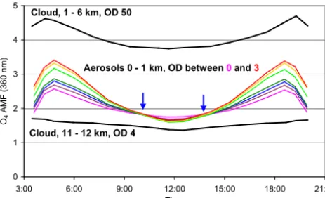
Figure 5.Simulated O4AMFs (360 nm) for different aerosol and
cloud scenarios. The violet and red lines indicate results for min-imum and maxmin-imum AOD of 0 and 3 respectively. For clear-sky
conditions almost the same O4AMFs are obtained around SZA of
36◦(indicated by the blue arrows), independent from the assumed AOD. Depending on the cloud OD and the cloud height, clouds can either increase or decrease the O4AMF compared to clear-sky
con-ditions (Wagner et al., 2011). The simulations are performed for a day (26 June 2009) in the middle of the campaign.
Here DAMFi indicates the differential O4 AMF derived
from the spectral analysis of an individual measurement. AMFcal,i indicates the corresponding calibrated O4AMF.
In the following we describe how AMFFRS can be
de-termined. Figure 5 presents simulated O4 AMFs for (near)
zenith view for different cloud-free (coloured lines) and cloudy conditions (black lines). From these simulation re-sults, two important findings can be deduced.
a. Around SZA of 36◦(indicated by the blue arrows) the O4AMFs for the different aerosol scenarios are almost
the same.
b. For cloudy scenarios the O4 AMF can be either
de-creased or inde-creased compared to cloud-free scenarios: for low and optically thick clouds the O4AMFs are
en-hanced, while for high and optically thin clouds the O4
AMFs are decreased (Wagner et al., 2011).
The first finding indicates that clear-sky observations (around SZA of 36◦) can in principle be used for the calibra-tion of the O4measurements, even if the exact AOD is not
known. The second finding indicates that cloudy measure-ments (as identified by CI) should be removed before the cal-ibration is performed. Figure 6 presents a comparison of the measured O4DAMFs and simulated O4AMFs. Note that the
yaxes were shifted by 1.78, the final value derived for the O4
AMF of the FRS (see below). In the top panel all measure-ments are shown and in the bottom panel only measuremeasure-ments for clear-sky conditions are shown (the cloud filtering was performed using the CI as described in Wagner et al., 2014). Interestingly, not only for the cloud-filtered measurements, but for all measurements the minimum O4DAMFs are well
0.5 1 1.5 2 2.5 3 3.5
03:00 06:00 09:00 12:00 15:00 18:00 21:00
Time
S
im
u
la
te
d
O4
A
M
F
-1.28 -0.78 -0.28 0.22 0.72 1.22 1.72
M
e
a
s
u
re
d
O
D
A
M
F
4
Reihe1
Reihe2
Reihe3
Reihe4
Reihe5
Reihe6
Reihe7
o4_AMF_90
AOD 0 0.1 0.2 0.3 1 2 3
0.5 1 1.5 2 2.5 3 3.5
03:00 06:00 09:00 12:00 15:00 18:00 21:00
Time
S
im
u
la
te
d
O4
A
M
F
-1.28 -0.78 -0.28 0.22 0.72 1.22 1.72
M
e
a
s
u
re
d
O
D
A
M
F
4
Reihe1
Reihe2
Reihe3
Reihe4
Reihe5
Reihe6
Reihe7
o4_AMF_90
AOD 0 0.1 0.2 0.3 1 2 3
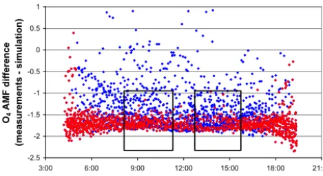
Figure 6.Comparison of measured O4DAMFs (right axis) with
simulated O4AMFs (left axis) for different AOD. In the top panel
all observations are shown and in the bottom panel only clear-sky observations are shown. The rectangles indicate the SZA ranges (30–50◦) used for the calibration of the O4measurements. The right yaxis is shifted compared to the leftyaxis by the O4AMF of the
FRS (−1.78). The measurements are from the period 12 June to 15 July 2009; the simulations are performed for a day (26 June 2009) in the middle of the campaign (aerosol layer height: 1000 m, surface albedo: 5 %).
represented by the simulations (for clear sky), indicating that during the CINDI campaign situations with only high thin cloud layers did not occur. This finding is confirmed by re-sults from lidar measurements (see Wagner et al., 2014). Of course, the probability of high clouds (without low clouds present at the same time) can be different for other seasons and locations. Thus we recommend that a cloud filter should always be applied to the measured O4DAMF, before they are
compared to the simulated O4AMFs.
Figure 7 presents the measured O4DAMFs after the
simu-lated O4AMFs for AOD of 0.2 were subtracted. This
normal-isation procedure is applied to remove the SZA dependence. The choice of the simulations for AOD of 0.2 is somehow arbitrary, but the exact choice has only a very small effect on the normalisation results. Polynomial expressions and tabu-lated values of the O4AMF for AOD=0.2 (clear-sky
-2.5 -2 -1.5 -1 -0.5 0 0.5 1
3:00 6:00 9:00 12:00 15:00 18:00 21:00
Time
O
A
M
F
d
if
fe
re
n
ce
4
(m
ea
su
re
m
en
ts
s
im
u
la
ti
o
n
)
Figure 7. Normalised O4DAMF for all measurements (blue) or
measurements under clear-sky conditions (red). The normalisation
is performed by subtracting the simulated O4 AMFs for AOD of
0.2. The rectangles indicate the SZA ranges used for the calibration
of the O4DAMF. The measurements are from the period 12 June to
15 July 2009.
For the calibration of the O4 DAMF, measurements for
SZA between 30 and 50◦were chosen for two reasons. a. For different aerosol layer heights, the SZA for which
the O4 AMF for different AOD become similar varies
slightly between about 30◦(for layer heights of 500 m)
and 50◦ (for layer heights of 2000 m), see Fig. A1 in the Appendix. Since the aerosol layer height is usually unknown and can vary with time, we chose a SZA range which covers typical aerosol layer heights.
b. After applying the cloud filter, the number of measure-ments decreased by about a factor of 3. The rather large SZA range ensures that a useful number of measure-ments is still available for the comparison with the sim-ulation results.
In Fig. 8 the frequency distribution of the normalised O4
DAMF is shown for all observations (blue) or only clear-sky observations (red). The maximum values and uncertainties are determined in the same way as for the CI (Sect. 2). For both cases (all measurements or clear-sky measurements) a value for the O4AMF of the FRS (AMFFRS)of 1.78 is
de-rived. The uncertainties are ±0.09 and ±0.08 for all and clear-sky observations respectively. Here it should be noted that the rather large uncertainties are caused by the low num-ber of observations and can probably be reduced if measure-ments for longer periods with more clear days are analysed. In the original version of our algorithm (Wagner et al., 2014) AMFFRS was determined based on selected clear-sky days
with similar AOD. In spite of the different procedures, a very similar value for AMFFRS(1.75) was found.
In Fig. 8 results for MAX-DOAS observations at Wuxi (China) are also shown (Wang et al., 2015). Measurements over a period from 1 January to 31 December 2012 were used. As for the Cabauw measurements, a clear peak is found indicating that the method works in a similar way for
com-0 0.05 0.1 0.15 0.2
-2 -1.5 -1 -0.5 0 0.5 1 1.5 2
Difference of measured O4 DAMF and simulated O4 AMF
R
el
at
iv
e
fr
eq
ue
nc
y
Reihe1 Relative frequency rel_fraction
All measurements
Clear sky Clear sky (Wuxi)
Figure 8.Frequency distribution (for bins of 0.05) of the normalised
O4DAMF for SZA between 30 and 50◦. The blue and red curves
represent observations at Cabauw for all sky conditions (896 mea-surements) and clear-sky conditions (302 meamea-surements) respec-tively. For both selections the frequency maximum is found for −1.78. The black curve represents the frequency distribution for
clear-sky observations at Wuxi (790 measurements).
pletely different locations and measurement conditions. The derived value for the O4AMF of the FRS is almost the same
as for the Cabauw measurements as both FRS were recorded at similar AOD and SZA.
Finally, two important aspects should be mentioned. a. For long-term measurements, it might be necessary to
use different FRS for different parts of the whole time series. In such cases the calibration procedure has to be applied for each selected FRS.
b. The O4VCD depends on atmospheric temperature and
pressure. Thus it varies with time. Depending on the weather conditions and season, such changes can ex-ceed 10 %. The variation of the O4 VCD leads to a
similar variation of the measured O4DAMFs. In
addi-tion, the temperature dependence of the O4cross section
probably further increases this variability. So far, these effects are not explicitly considered in most studies, and here we also assumed the O4VCD to be constant. Thus
part of the scatter of the measured O4AMFs in Figs. 7
and 8 might be caused by the variation of the O4VCD
and temperature dependence of the O4 cross section.
However, the current version of the algorithm is only slightly affected by the corresponding uncertainties of the derived O4DAMFs, because they are used only for
the identification of optically thick clouds and fog. Fu-ture studies might take the effects discussed above into account when retrieving the O4DAMFs from the
Clear sky, low aerosol
Continuous clouds
Smooth temp. var. of CIZ
andspread of CI for
different elevation angles
Clear sky, high aerosol CIZ,meas< Ciref?
CI the same for all elevation angles ?
Broken clouds
Rapid temp. var. of CI ?Z
YesNo Clear sky betw.
clouds
Fog
Thick clouds (continuous or
broken)
O4the same for all
elevation angles ?
O4,Z> O4,ref ?
Rapid temp. var.
of CIZ ?
(TSI > TSIref ?)
YesNo
Yes
Yes
Yes
Yes
Yes 2
2
3 3 1 1
4 4
8 8
cloud infl. for indiv. meas. CI for other elevation angles
vary rapidly ? yes
5 5
6 6
7 7
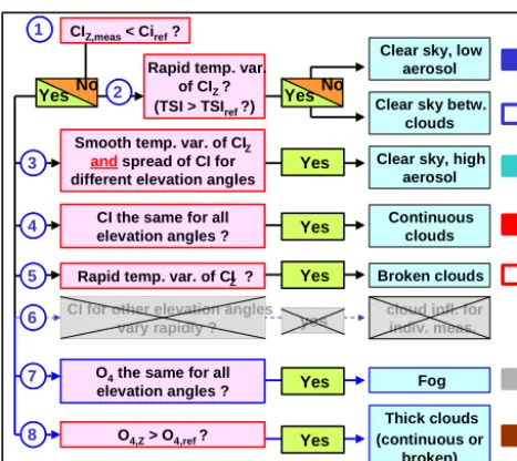
Figure 9.Flow chart of the updated cloud classification scheme. The basic structure is the same as in the original scheme (Fig. 14 in Wagner et al., 2014). However, except for the decision criterium for fog (decision no. 7), all other criteria were changed compared to the original scheme. The individual changes are summarised in Table 1. For decision no. 6, no universal recommendation can be given, be-cause the spread of the non-zenith angles depends in particular on the relative azimuth angle. Thus it is omitted in the updated classi-fication scheme.
4 Update of the cloud classification scheme using the newly calibrated MAX-DOAS CI and O4data
Wagner et al. (2014) developed a scheme for the classifica-tion of cloud and aerosol condiclassifica-tions based on MAX-DOAS measurements. In this section we introduce an updated ver-sion of this classification scheme. Compared to the original version, four major changes are applied.
a. The threshold values of the original scheme have been adapted to the newly calibrated CI and O4data.
b. The new threshold values are based on well-defined at-mospheric conditions. Thus the procedures for the de-termination of the threshold values can be applied to any measurements at different locations and seasons. The new threshold values also better represent the SZA dependencies.
c. The threshold values are also provided for the new CI. d. The determination of optically thick clouds is only
based on O4measurements (without making use of the
radiance measurements).
The basic scheme of the original classification algorithm, however, is not changed. For most of the individual decision steps the normalisation procedures and the definition of the
threshold values for the involved quantities were adapted. An overview on the new classification scheme and the applied changes is provided in Fig. 9 and Table 1. Only for the identi-fication of fog, are exactly the same criteria as in the original algorithm still used. For the other quantities the new thresh-olds were chosen to best match those of the original scheme. The individual changes are summarised in Table 1 and are discussed in detail in the next subsections. At the end of this chapter (Sect. 4.6) the results of the new scheme are com-pared to the results of the original scheme.
4.1 New threshold values for the CI
In the original cloud classification scheme the measured CI was first normalised (divided) by a SZA-dependent clear-sky reference value (simulated for an AOD of 0.3). The normal-isation was applied to correct the strong SZA dependence of the CI (see Fig. 1). Then a constant threshold (indepen-dent of the SZA) was used to discriminate clear from cloudy observations. However, it turned out that the simple normal-isation was not sufficient for large SZA (>60◦). Thus we decided to use a SZA-dependent threshold in the new ver-sion of our cloud classification algorithm (but we not apply the normalisation of the measured CI values anymore). As threshold values, we use simulation results for AODs of 0.75 for 440 nm (CIorig)and 0.85 for 390 nm (CInew)respectively.
The AOD value of 0.75 at 440 nm was chosen to achieve consistency between the new and the original classification scheme (for small SZA). The corresponding AOD values at the other wavelengths (including those for the calculation of CInew)were derived from the AOD at 440 nm using a typical
Ångstrøm exponent of unity.
In Fig. 10 the calibrated CIorig and CInew for 24 June
2009 are compared to simulated CI for different aerosol and cloud properties. Note that the CI for AOD of 0.85 at 390 nm represents the SZA-dependent threshold value, see Tables 1 and A1. During the morning the measured CI are similar to the simulation results (blue lines) for the AOD obtained from the simultaneous AERONET measurements. Around noon, the AOD increases and some clouds also appear. As a consequence the measured CI decreases and it even falls slightly below the simulated minimum values several times. After about 15:00 the clouds disappear, but the CI stays at low levels because of the increased AOD in the afternoon.
Polynomial expressions describing the SZA-dependent threshold values for zenith viewing direction are provided in Table 1; tabulated values are provided in Table A1 in the Ap-pendix.
4.2 New threshold values for the temporal smoothness indicator (TSI)
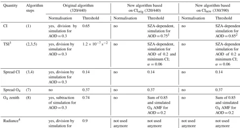
Table 1.Comparison of the normalisation procedures and threshold values for the individual decisions of the cloud classification scheme of the original algorithm and the new algorithms (for CIorigand CInew). In the column “algorithm steps” it is indicated in which decisions the
selected quantity is involved (see Fig. 9).
Quantity Algorithm Original algorithm New algorithm based New algorithm based
steps (320/440) on CIorig(320/440) on CInew(330/390)
Normalisation Threshold Normalisation Threshold Normalisation Threshold
CI (1) yes, division by
simulation for
AOD=0.3
0.65 no SZA-dependent,
simulation for
AOD=0.751
no SZA-dependent,
simulation for
AOD=0.852
TSI3 (2,3,5) yes, division by
simulation for
AOD=0.3
1.2×10⁻⁷s−2 no SZA-dependent,
simulation for AOD of 0.2 and minimum CI;
α=0.06
no SZA-dependent,
simulation for AOD of 0.2 and minimum CI;
α=0.06
Spread CI (3,4) yes, division by
simulation for
AOD=0.3
0.14 no 0.14 no 0.14
Spread O4 (7) no 0.37 no 0.37 no 0.37
O4zenith (8) yes, subtraction
of simulation for
AOD=0.3
0.74 no Sum of 0.85
and simulated
O4AMF for
AOD=0.2
no Sum of 0.85
and simulated
O4AMF for
AOD=0.2
Radiance4 yes, division by
simulation for
AOD=0.3
0.9 not used
anymore
not used anymore
not used anymore
not used anymore
1AOD for 440 nm;2AOD for 330 nm;3The definition of TSI has changed: for the new TSI no time information is used (see text).4In the new scheme optically thick clouds are identified by
the O4absorption alone.
to identify rapid variations of the sky conditions, e.g. related to broken clouds. In our original study, the time differences between the individual measurements were explicitly con-sidered for the calculation of the TSI. In fact, the TSI was defined as the discrete approximation of the second deriva-tive in time. The TSI was also normalised (divided) by the clear-sky reference value and a constant threshold was ap-plied to discriminate measurements with high TSI from mea-surements with low TSI (indicating a smooth temporal vari-ation of the CI). In the new version two important changes are applied: first, the time difference between the individual measurements is not considered anymore for the calculation of the TSI. The motivation for this change is the fact that the TSI (as defined in Eq. 7 in Wagner et al., 2014) depends strongly on the time differences between individual measure-ments and thus on the individual instrument properties and measurement protocols. For practical use in MAX-DOAS in-versions it is, however, sufficient to know whether the sky condition has changed during the time interval of a typical elevation sequence (independent from the actual duration of this elevation sequence). Thus, in the updated version of the cloud classification scheme, we use the following (simpler) definition of the TSI:
TSIn=
CI
n+1+CIn−1
2 −CIn
. (7)
Here CIn indicates the CI in zenith direction of thenth
el-evation sequence. Another change compared to the original classification scheme is that the TSI is not normalised by the clear-sky CI reference values, but instead a SZA-dependent threshold is used. The advantage of this approach is that the threshold values can be calculated based on well-defined at-mospheric scenarios. Here we suggest using the difference of the CI for a clear-sky scenario with moderate aerosol load (AOD of 0.2) and the minimum CI for cloudy conditions (see Fig. 10). The AOD of 0.2 is assumed for the upper wave-length and the AOD for the lower wavewave-length is calculated assuming an Ångström exponent of 1. The threshold value is calculated from the CI for both scenarios:
TSIthreshold(SZA)=α×CIdiff(SZA)= (8)
α× [CIAOD=0.2(SZA)−CImin(SZA)].
Here TSIthreshold(SZA) represents the threshold value and
CIdiff(SZA) is the difference of the simulated CI for clear and
cloudy conditions. We chose the proportionality constantα
such that for SZA around 50◦the threshold value for the new version of the algorithm matches that of the original version. The best agreement is found forα=0.06 (see Fig. 11). The polynomial expression for CIdiff (SZA) for the exact zenith
0.0 0.5 1.0 1.5 2.0 2.5
03:00 06:00 09:00 12:00 15:00 18:00 21:00
Time
C
I
I(
32
0
nm
)
/
I(
44
0
nm
)
Reihe6 Reihe3 Reihe1 Reihe9 Reihe5
Measurements
AOD: 0 AOD: 0.13 AOD: 0.75
Minimum
0.0 0.4 0.8 1.2 1.6 2.0
03:00 06:00 09:00 12:00 15:00 18:00 21:00
Time
C
I
I(
33
0
nm
)
/
I(
39
0
nm
)
Reihe6 Reihe3 Reihe2 Reihe9 Reihe5
Measurements
AOD: 0 AOD: 0.16 AOD: 0.85
Minimum
Figure 10. Comparison of measured normalised CI for 24 June 2009 with simulated CI for different scenarios. Top: original CI for 320 and 440 nm; Bottom: new CI for 330 nm/390 nm. The AOD val-ues in the legends correspond to the wavelengths 440 and 390 nm respectively. The blue curves represent CI for the AOD measured by the AERONET instrument on the morning of 24 June 2009. The red curves represent CI for the threshold values used in the new classi-fication scheme. The minimum values represent cloudy conditions (see Fig. 1). The simulations are made for a day (26 June 2009) in the middle of the campaign.
have to be multiplied byα=0.06 before they can be used as threshold value for the new TSI.
In this study, we do not provide a set of thresholds for the TSI in non-zenith viewing directions, because they also de-pend on the azimuth angle, which is different for different instruments (and seasons).
4.3 Threshold values for the spread of the CI for different elevation angles
The spread of the CI for the different elevation angles ap-proaches zero in the presence of clouds (Wagner et al., 2014), which makes it a useful quantity for the distinction between situations with enhanced aerosol loads or clouds. In addition, the spread of the CI can be used to identify clouds at low SZA, when identification by the absolute value of the CI fails (see Wang et al., 2015). The spread of the CI is calculated as the difference between the maximum and minimum CI for all elevation angles of an individual elevation sequence. Wagner
(a)
0 0.5 1 1.5
C
I (
I320 /I44
0
) CI (I320/I440)
(b)
0E+0 4E-7 8E-7
4:00 6:00 8:00 10:00 12:00 14:00 16:00 18:00
T
S
I
(I32
0
/I440
) TSI
old (I320/I440)
(c)
0 0.1 0.2 0.3
4:00 6:00 8:00 10:00 12:00 14:00 16:00 18:00
T
S
I (
I320 /I44
0
) TSInew (I320/I440)
(d)
0 0.1 0.2
04:00 06:00 08:00 10:00 12:00 14:00 16:00 18:00 Time
T
S
I
(I33 0/I
3
9
0
) TSI
new (I330/I390)
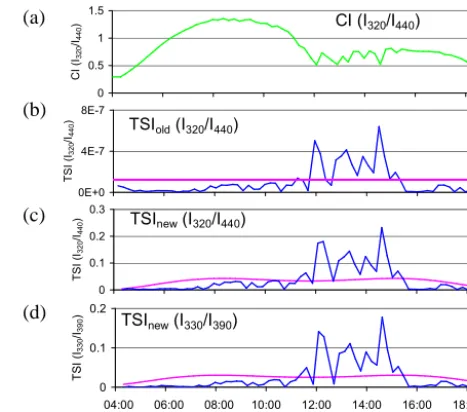
Figure 11. (a) Measured normalised CI (a) for 24 June 2009. (b)Normalised TSI according to the original algorithm. Here a con-stant threshold value was used.(c, d)New TSI as used in this study without normalisation and explicit consideration of the time (Eq. 7). The threshold values for the new TSI depend on the SZA.
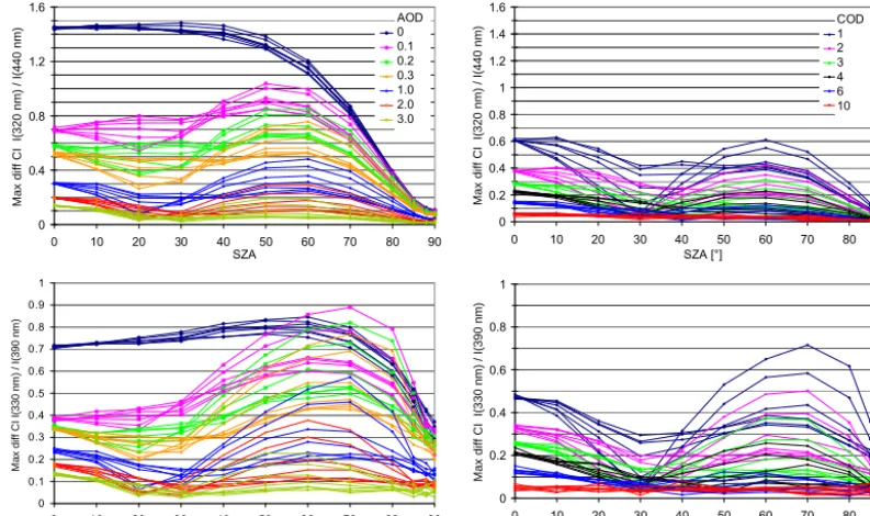
et al. (2014) performed simulations of the spread of the CI for selected relative azimuth angles only. Here we extended these calculations to cover all relevant combinations of rel-ative azimuth angles and SZA (see Fig. 12). Based on these results the following can be concluded.
a. No clear SZA dependence is found. Thus a simple nor-malisation as a function of the SZA (as in Wagner et al., 2014) is in general not appropriate, and in the new version of the classification scheme no normalisation as function of the SZA is performed. We keep the original threshold value of 0.14 (see Table 1), because accord-ing to Fig. 12 it still seems to be a good compromise to discriminate clouds and aerosols. Here it should be noted that for individual measurements (with a specific relation between the SZA and the relative azimuth an-gle) a monotonous relationship between the spread of the CI and the SZA might occur. In such cases a SZA-dependent threshold might still be useful.
b. Clouds and aerosols (with the same optical depth) have a very similar effect on the spread of the CI (the differ-ences are mainly a result of the different wavelength de-pendence of cloud and aerosol scattering). Thus in many cases, it is difficult to clearly discriminate between both types of atmospheric scatterers based on the spread of the CI.
0 0.4 0.8 1.2 1.6
0 10 20 30 40 50 60 70 80 90
SZA
M
a
x
d
if
f
C
I
I
(3
2
0
n
m
)
/
I(
4
4
0
n
m
) Reihe1
Reihe2 Reihe4 Reihe3 Reihe5 Reihe6 Reihe7
AOD 0 0.1 0.2 0.3 1.0 2.0 3.0
0 0.2 0.4 0.6 0.8 1 1.2 1.4 1.6
0 10 20 30 40 50 60 70 80 90
SZA [°]
M
a
x
d
if
f
C
I
I
(3
2
0
n
m
)
/
I(
4
4
0
n
m
)
320_440 Reihe2 Reihe3 Reihe4 Reihe5 Reihe6
COD 1 2 3 4 6 10
0 0.1 0.2 0.3 0.4 0.5 0.6 0.7 0.8 0.9 1
0 1 0 20 30 40 50 6 0 70 80 90
SZA
M
a
x
d
if
f
C
I
I(
3
3
0
n
m
)
/
I(
3
9
0
n
m
)
0 0.2 0.4 0.6 0.8 1
0 10 20 30 40 50 60 70 80 90
SZA [°]
M
a
x
d
if
f
C
I
I
(3
3
0
n
m
)
/
I(
3
9
0
n
m
)
Figure 12.Spread of the CI (top: CIorigfor 320 nm/440 nm; bottom: CInewfor 330 nm/390 nm) between the different elevation angles for
different aerosol (left) and cloud (right) scenarios. The spread is calculated as the difference between the maximum and minimum CI for a given combination of SZA and relative azimuth angle. The different lines of the same colour represent simulations for different relative azimuth angles (0, 30, 60, 90, 120, 150, 180◦). The simulations are made assuming an elevation angle of 85◦for zenith view. Results for exact zenith view are almost identical (see Fig. A2 in the Appendix).
the presence of clouds in situations (e.g. at small SZA) in which they can not be identified based on the zenith CI itself (Wang et al., 2015).
4.4 New threshold for the O4AMF in zenith direction
In contrast to the original version of the algorithm, the SZA dependence of the measured O4 AMFs is not corrected by
subtracting the corresponding clear-sky reference values in the new algorithm. Instead, the measured O4AMFs are
com-pared to the wavelength-dependent clear-sky reference value, to which a constant offset is added (representing the effect of multiple scattering inside optically thick clouds). In contrast to the original classification scheme, the clear-sky reference value is calculated for an AOD of 0.2 (instead of 0.3) to be consistent with the AOD measured by the AERONET sun photometer on 24 June 2009, which was chosen as a clear-sky reference. Because of the new O4calibration and the new
clear-sky reference values a slightly different offset (0.85) compared to the original version (0.74) was chosen in order to bring the results of the new algorithm into close agree-ment with those of the original algorithm. A comparison of the measured (calibrated) O4AMF with the threshold value
for a day with occasional optically thick clouds is shown in Fig. 13.
0 2 4
03:00 05:00 07:00 09:00 11:00 13:00 15:00 17:00 19:00
Figure 13. Measured O4 AMF (blue, after normalisation) for
15 June 2009. The magenta curve represents the SZA-dependent threshold.
4.5 Threshold for the spread of the O4AMF
The calculation of the spread of the O4AMF for the different
elevation angles is not affected by the new calibration, since the same offset value is added to the O4DAMF of all
eleva-tion angles. Thus, the same threshold value as in the original version (0.37) is still used.
4.6 Comparison of the results of the original and the new classification schemes
We applied the updated classification scheme (using ei-ther CIorig or CInew)to the same data set as in Wagner et
0 % 20 % 40 % 60 % 80 % 100 % 0 % 20 % 40 % 60 % 80 % 100 %
SZA: 70°–85°
SZA: 28°–70°
Old yes New yes Old yes New no Old no New no Old no New yes
Clear, low Clear, high aerosols aerosols
Cloud holes
Continous clouds
Broken clouds
Fog Thick clouds 1 2 1 2 1 2 1 2 1 2 1 2 1 2 1 2 1 2 1 2 1 2 1 2 1 2 1 2 1: CI 320 / 440 nm
2: CI 330 / 390 nm
Figure 14. Comparison of the results of the original and updated classification scheme. The black numbers indicate the comparison results between the original algorithm and the updated algorithm
using CIorig (1) and between the original algorithm and the
up-dated algorithm using CInew(2). Blue and red colours represent
cases which were assigned or not assigned to the respective class by the original algorithm. Bars with full colours indicate agreement between the old and new algorithm, hatched bars indicate disagree-ment between the old and new algorithm.
substantial deviations for particular classification results also occur. These differences are mainly caused by the different treatment of the normalisation and the SZA dependence of the thresholds, in particular those for the absolute value of the CI (step no. 1 in Fig. 9). Due to this change, much fewer mea-surements for SZA>70◦are assigned to the class “clear sky with low aerosol” than in the original classification scheme. This change, however, seems to be reasonable, since for the new algorithms the relative fraction of the class “clear sky with low aerosol” has become more similar for low and high SZA. The updated threshold for the CI also leads to a con-siderable shift of cases from the class “cloud holes” to the class “broken clouds”. This change also seems to be reason-able, because the results of the new algorithm for both classes have become more similar for low and high SZA, especially for the new CI.
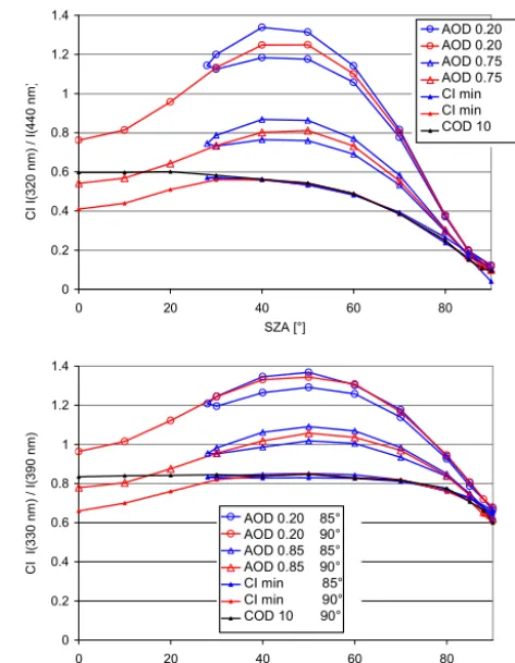
4.7 Threshold values for observations at exactly zenith direction (elevation angle of 90◦)
Since the zenith observations were not performed in exact zenith direction (but instead at an elevation angle of 85◦)
for our MAX-DOAS measurements during the CINDI cam-paign, the question arises as to whether the threshold values can also be used for observations in exact zenith direction. In Fig. 15 the threshold values for the CI (based on the de-fined atmospheric scenarios) are compared for elevation an-gles of 85 and 90◦. The differences of the CI are typically
<10 % (the minimum values are almost identical). Thus we
0 0.2 0.4 0.6 0.8 1 1.2 1.4
0 20 40 60 80
SZA [°]
C
I I
(3
20
n
m
)
/ I
(4
40
n
m
)
320_AE1 CI_320_440_AE1 320_AE1 CI_320_440_AE1 CI_330_390_min CImin_320_440 CI_OD_10_320_440 AOD 0.20 85° AOD 0.20 90° AOD 0.75 85° AOD 0.75 90° CI min 85° CI min 90° COD 10 90°
0 0.2 0.4 0.6 0.8 1 1.2 1.4
0 20 40 60 80
SZA [°]
C
I
I(
33
0
nm
)
/ I
(3
90
n
m
)
330_AE1 CI_320_440_AE1 320_AE1 CI_320_440_AE1 CI_330_390_min CImin_320_440 CI_OD_10_320_440 AOD 0.20 85° AOD 0.20 90° AOD 0.85 85° AOD 0.85 90° CI min 85° CI min 90° COD 10 90°
Figure 15. Comparison of simulated CI (top: CIorig:
320 nm/440 nm; bottom: CInew: 330 nm/390 nm) for elevation
angles of 85◦ (blue lines) and 90◦ (red lines). The different
symbols represent different atmospheric scenarios. The black line represents results for a cloud optical depth of 10.
0 0.5 1 1.5 2 2.5 3
0 10 20 30 40 50 60 70 80 90
SZA [°]
O
4
A
M
F
3
60
n
m
(
A
O
D
=
0.
2)
Reihe1 Reihe2
85° 90°
Figure 16.Comparison of the clear-sky reference values of the O4 AMF for elevation angles of 85 and 90◦.
an-gles of 85 and 90◦are compared. Almost identical values are found, indicating that the reference value for 85◦ can also
be used for measurements at exactly zenith view. Polynomial expressions for all threshold values for exact zenith direction are provided in Table 2; tabulated values are provided in Ta-ble A1 in the Appendix.
5 Further improvements of the classification scheme
In this section possible extensions and improvements of the calibration procedure and classification scheme are dis-cussed.
5.1 Effect of instrumental degradation for long-term measurements
Especially for long-term measurements, instrumental degra-dation can become an important issue, because the results of the CI, O4absorption (and radiance) might systematically
change over time. Wang et al. (2015) presented a method to quantify the effect of instrument degradation using time se-ries of the derived quantities. They also suggested a degra-dation correction for the observed CI and radiance. Unfor-tunately, the effect of instrumental changes for the O4
ab-sorption (in particular the change of the instrument’s reso-lution) can be very strong, and these influences cannot usu-ally be corrected well. In such cases, the O4absorption can
not be used for the detection of optically thick clouds. Thus, for long-term observations the occurrence of optically thick clouds should probably be based on observations of the radi-ance. An approach for an indirect calibration of the radiance will be proposed in Sect. 5.2.
5.2 Estimation of a SZA-dependent threshold for the radiance
Optically thick clouds can be identified using the O4
absorp-tion or the measured radiance (Wagner et al., 2014). Espe-cially for long-term measurements, the effect of instrumen-tal degradation on the radiance is usually much weaker than for the retrieved O4absorption (see e.g. Wang et al., 2015).
However, as mentioned before, the calibration of the radi-ance requires more effort than the calibration of the CI and O4 absorption. In particular, measurements for days with
constant and well-known AOD are required (Wagner et al., 2015). Thus, the updated version of the cloud classification scheme does not use the measured radiance for the detection of optically thick clouds, because such clouds can also be clearly identified by the O4absorption observed in zenith
di-rection. Nevertheless, especially for long-term observations, the use of O4observations for the detection of optically thick
clouds might be strongly affected by instrumental degrada-tion (Wang et al., 2015). For such cases it might still be useful to identify optically thick clouds based on the measured ra-diance. Thus, in this subsection we propose a simple method
0E+00 1E+07 2E+07 3E+07 4E+07 5E+07 6E+07
03:00 06:00 09:00 12:00 15:00 18:00 21:00
Time
S
ig
n
a
l [
co
u
n
ts
se
c
]
Thin clouds Thick clouds
–1
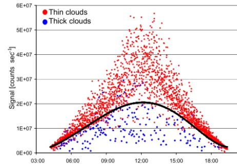
Figure 17.Measured radiance at 360 nm (in units of counts s−1) for near-zenith observations during the Cabauw campaign. The blue/red dots indicate measurements which were classified as un-der optically thick/thin clouds, based on the calibrated O4
absorp-tion using the updated thresholds. The black curve represents the threshold value for the radiance used in the original version of the algorithm. The measurements are from the period 12 June to 15 July 2009.
for the determination of a threshold value which can be ap-plied to the uncalibrated radiance. It is based on the compari-son of measured radiances for optically thick and thin clouds as determined from the O4absorption. In Fig. 17 all radiance
observations for optically thin clouds (identified by the O4
absorption) are indicated by red dots and measurements for optically thick clouds by blue dots. In spite of some outliers, the transition between thin and thick clouds (as a function of the SZA) can be clearly identified. Moreover, the threshold value used in the original version of the algorithm (indicated by the black line) fits well to the transition between the red and blue points. This finding indicates the possibility of de-termining the threshold value for the radiance without per-forming an explicit radiance calibration of the instrument via the relationship with the observed O4 absorption in zenith
direction. This method could be applied for periods in which the effect of instrumental changes on the O4absorption are
negligible. The derived radiance calibration could then be used for the entire period of the MAX-DOAS measurements.
5.3 Observations at low latitudes
The results in Fig. 15 indicate a potential problem for mea-surements at low SZA (<30◦). For such viewing geometries,
iden-Table 2.Polynomial expressions for the different SZA-dependent clear-sky reference and threshold values.
Function in
classification scheme
Quantity Scenario Polynomial as function of the normalised SZA
(S=SZA/90◦) Clear-sky reference
value
CInew
(330 nm/390 nm)
AOD=0.2 =8.399×S6−24.253×S5+29.143×S4−21.056×
S3+7.673×S2−0.197×S+0.964
Threshold value CInew
(330 nm/390 nm)
AOD=0.85 = −0.654×S6+0.367×S5+2.647×S4−6.006×S3+
3.576×S2−0.094×S+0.779
Minimum value CInew
(330 nm/390 nm)
cloudy sky = −5.261×S6+8.045×S5+0.621×S4−6.588×S3+
3.029×S2+0.09×S+0.66
Difference between clear and cloudy sky1
TSI for CInew
(330 nm/390 nm)
CIdiffas defined in
Eq. (8)
=13.66×S6−32.298×S5+28.522×S4−14.468×
S3+4.644×S2−0.288×S+0.304
Clear-sky reference value
CIorig
(320 nm/440 nm)
AOD=0.2 =22.785×S6−54.778×S5+53.783×S4−33.961×
S3+12.088×S2−0.563×S+0.762
Threshold value1 CIorig
(320 nm/440 nm)
AOD=0.75 =11.216×S6−25.441×S5+22.575×S4−13.89×
S3+5.313×S2−0.221×S+0.542
Minimum value CIorig
(320 nm/440 nm)
cloudy sky =18.635×S6−57.262×S5+67.785×S4−39.153×
S3+10.144×S2−0.472×S+0.41
Difference between clear and cloudy sky1
TSI for CIorig
(320 nm/440 nm)
CIdiffas defined in
Eq. (8)
=4.15×S6×+2.484×S5−14.002×S4+5.191×S3+
1.944×S2−0.09×S+0.352
Clear-sky reference value2
O4AMF zenith AOD=0.2 = −81.975×S6+197.773×S5−172.649×S4+
64.482×S3−7.832×S2+0.964×S+1.265
1For use as threshold for the TSI, the polynomial has to be multiplied by a factorα=0.06(see Eq. 8).2For use as threshold for the O
4AMF, a value of 0.85 has to be added to the polynomial.
tify clouds by the spread of the CI as proposed by Wang et al. (2015).
5.4 Possible ways of distinguishing between the effects of clouds and aerosols with similar optical depths
As discussed in Sect. 4.3, from measurements of the absolute value of the CI alone it is difficult to distinguish between aerosols and clouds if they have the same optical thickness (especially for optical thicknesses between about 1 and 6). This is especially important for the presence of continuous clouds, because they cannot be detected by enhanced values of the temporal smoothness indicator.
We recommend making use of the O4observations to
dis-tinguish between aerosols and continuous clouds. We suggest the following two approaches.
a. If clouds are not included in the forward model for the aerosol profile inversion of MAX-DOAS retrievals, continuous clouds might be simply identified by the bad convergence (large differences between the measured O4absorptions and the corresponding results) of the
for-ward model.
b. More sophisticated versions of the forward model might even include a simple parameterisation of clouds (e.g.
based on homogenous clouds with different optical depths and altitudes). Homogenous clouds might then simply be identified by the retrieved layer height (if they is larger than the typical aerosol layer height).
These possibilities should be investigated in further stud-ies.
5.5 Observations at high latitudes and over bright surfaces
The application of the cloud classification scheme at high latitudes is subject to two specific problems. First, measure-ments at small SZA are rare. This problem mainly affects the calibration of the O4absorption. Second, the surface will be
covered by snow and ice during large parts of the year. Here it should be noted that, also at midlatitudes, the surface might be covered by ice and snow during part of the year. Increased values of the surface albedo strongly affect the atmospheric radiative transport and thus probably also the proposed cali-bration approaches and derived threshold values.
Figure 18 shows simulated CI and O4AMFs in zenith
0 0.5 1 1.5
0 20 40 60 80
SZA [°]
C
I
I(
3
3
0
n
m
)
/ I
(3
9
0
n
m
)
Reihe1 Reihe3 Reihe4
AOD 0.20 90°, alb. 0.80 AOD 0.85 90°, alb. 0.80 COD 10 90°, alb. 0.80
0 1 2 3 4
0 20 40 60 80
SZA [°]
O4
A
M
F
Surface albedo: 5 %
0 1 2 3 4
0 20 40 60 80
SZA [°]
O4
A
M
F
Reihe1 Reihe2 Reihe3 Reihe4 Reihe5 Reihe6 Reihe7
AOD: 0 0.1 0.2 0.3 1.0 2.0 3.0 Surface albedo: 80 %
Figure 18.Top: simulated CI for zenith direction for clear-sky
mea-surements above bright surfaces (albedo=80 %). Middle and
bot-tom: simulated O4 AMF for low (5 %) and high (80 %) surface albedo. The different colours indicate results for different AOD.
an almost constant value, indicating the effect of increased multiple scattering, which also leads to more Rayleigh scat-tering events of the observed photons. These results indicate that for measurements over snow- and ice-covered surfaces a similar calibration approach for the CI as for measurements over low albedo can be applied.
In contrast, the O4AMFs (Fig. 18, bottom) are strongly
affected by the increased surface albedo. Compared to the results for low surface albedo, systematically higher values are found. Moreover, for SZA<80◦, the O4 AMF depends
strongly on the AOD. We made additional simulations for different values of the surface albedo between zero and unity (see Fig. A3 in the Appendix). Interestingly, for all values a specific SZA exists, for which the O4AMFs become
inde-pendent from the AOD. The dependence of this SZA on the surface albedo is almost linear (see Fig. 19).
From these findings we conclude that the calibration method developed for measurements above small surface albedo has to be modified before it can be applied to mea-surements over high surface albedo. Clear-sky meamea-surements at large SZA can probably be used for the comparison of measured and simulated O4AMF. Fortunately, this
possibil-0 20 40 60 80
0 0.2 0.4 0.6 0.8 1
Surface albedo
S
Z
A
[
°]
Figure 19.SZA, for which the O4absorption becomes independent from the aerosol optical depth as function of the surface albedo (see also individual simulation results in Fig. A3 in the Appendix).
ity fits well to the fact that at high latitudes most measure-ments are performed at moderate to high SZA.
These simulation results indicate that for measurements over bright surfaces modified calibration approaches and threshold values would have to be used. These modifications need to be tested in more detail. Here it should also be con-sidered that the surface albedo often changes rapidly, espe-cially in spring and autumn. Thus methods for the detection (and quantification) of changes of the surface albedo based on the MAX-DOAS observations should also be developed.
6 Conclusions and outlook
We developed methods for the calibration of the colour index (CI) and the O4absorption derived from MAX-DOAS
mea-surements of scattered sunlight, which are an important step towards a universal cloud classification scheme for MAX-DOAS observations. Both calibration methods are based on the comparison of measurements and radiative transport sim-ulations for well-defined atmospheric conditions (e.g. clear or cloudy conditions) and limited SZA ranges. It should be noted that, except for the determination of the spread of the CI and the O4absorption (see Fig. 9), the algorithm can also
be applied to “traditional” zenith sky DOAS instruments. For the calibration of the CI, observations under cloudy conditions are used, for which minimum values of the CI are found (if the CI is defined as the ratio of the intensity at the short wavelength divided by the intensity at the long wave-length). The result of the calibration procedure is a propor-tionality constant, which is applied to the measured CI.
For the calibration of the O4absorption observations under
clear-sky conditions and for a limited SZA range are used. As a result of the calibration procedure a constant offset is determined (the O4 absorption of the Fraunhofer reference
spectrum), which is added to the measured O4 absorption.
In the second part of our study we applied the cloud clas-sification algorithm described in Wagner et al. (2014) to the calibrated CI and O4 absorptions and adapted the original
threshold values accordingly. Together with the calibration method, the new set of threshold values can be used in a con-sistent way for any MAX-DOAS measurement thus consti-tuting a universal method for cloud classification. In addition to the new threshold values, the updated version of the cloud classification includes further important improvements.
a. We used a new wavelength pair (330 nm/390 nm) for the CI. Compared to the CI (320 nm/440 nm) used in our original study (Wagner et al., 2014) this choice has two advantages: the change of the low wavelength to 330 nm largely minimises the impact of the ozone absorption on the CI. The change of the upper wavelength to 390 nm ensures that the new CI can be calculated for almost all UV (MAX-)DOAS instruments (which often do not cover 440 nm).
b. The new threshold values better describe the SZA dependence. They are obtained from radiative trans-fer simulations for well-defined atmospheric scenarios. This aspect is important, since it ensures that thresh-old values for possible modified CI or additional cloud-sensitive quantities could be determined in a consistent way (based on the same atmospheric scenarios). c. No radiance measurements are used in the new version,
because the absolute calibration of the measured radi-ance spectra is more complicated than those of the CI and the O4absorption. Fortunately, the omission of the
radiance measurements has no large impact on the clas-sification results, because the radiance was only used for the detection of optically thick clouds, which can also be identified from the O4absorption.
We compared the results of the updated cloud classifica-tion scheme with those from the original version and found general good agreement. The comparison results indicate that the updated classification scheme yields more consistent results for high SZA (>70◦) than the original classification scheme.
It should be noted that our cloud classification algorithm is optimised for MAX-DOAS measurements at midlatitudes.
For measurements at high and low latitudes specific prob-lems occur: at low latitudes, many measurements are per-formed for small SZA, for which the CI becomes indistin-guishable for clear and cloudy conditions. As suggested by Wang et al. (2015) this problem can be partly overcome by the use of the spread of the CI for the identification of clouds. At high latitudes, measurements at small SZA are rare, which can lead to problems for the application of the calibration methods, especially for the O4absorption. In
ad-dition, frequently increased surface albedo due to snow and ice strongly affect the atmospheric radiative transfer and thus the prerequisites of our calibration methods. However, sensitivity studies suggest that for such conditions modified versions of the calibration methods and cloud classification scheme can still be applied.
Another problem with the new version of the algorithm is that, especially for long-term observations, the derived O4
absorptions might be strongly affected by temporal changes of the instrument properties. Thus, the identification of op-tically thick clouds might be impossible for such measure-ments. As a possible solution for this limitation we propose a new indirect determination of the threshold value for the un-calibrated radiance, which is based on the O4measurements
for periods which are not affected by instrumental changes. Optically thick clouds could then be identified based on the uncalibrated radiances, which are usually less affected by in-strument degradation (and can be better corrected for instru-mental changes than the O4absorption).
Finally we identify important research areas, which should be addressed in future studies in order to further improve the cloud classification scheme. These areas include a more so-phisticated use of CI from individual elevation angles (in-stead of simply using the spread of the CI), modifications for the cloud classification algorithm for situations with high surface albedo, an improved discrimination of clouds and aerosols based on O4absorptions as well as the investigation
of 3-D cloud effects on the CI.
7 Data availability