www.atmos-meas-tech.net/5/2469/2012/ doi:10.5194/amt-5-2469-2012
© Author(s) 2012. CC Attribution 3.0 License.
Measurement
Techniques
1 km fog and low stratus detection using pan-sharpened MSG
SEVIRI data
H. M. Schulz1, B. Thies1, J. Cermak2, and J. Bendix1
1Laboratory for Climatology and Remote Sensing, Faculty of Geography, Philipps-University, Marburg, Germany 2Institute of Geography, Ruhr University Bochum, Bochum, Germany
Correspondence to: H. M. Schulz ([email protected])
Received: 30 March 2012 – Published in Atmos. Meas. Tech. Discuss.: 26 June 2012 Revised: 24 September 2012 – Accepted: 25 September 2012 – Published: 22 October 2012
Abstract. In this paper a new technique for the detection of fog and low stratus in 1 km resolution from MSG SEVIRI data is presented. The method relies on the pan-sharpening of 3 km narrow-band channels using the 1 km high-resolution visible (HRV) channel. As solar and thermal channels had to be sharpened for the technique, a new approach based on an existing pan-sharpening method was developed using local regressions. A fog and low stratus detection scheme origi-nally developed for 3 km SEVIRI data was used as the basis to derive 1 km resolution fog and low stratus masks from the sharpened channels. The sharpened channels and the fog and low stratus masks based on them were evaluated visually and by various statistical measures. The sharpened channels devi-ate only slightly from reference images regarding their pixel values as well as spatial features. The 1 km fog and low stra-tus masks are therefore deemed of high quality. They contain many details, especially where fog is restricted by complex terrain in its extent, that cannot be detected in the 3 km reso-lution.
1 Introduction
Fog and low stratus (FLS) have operationally been detected from AVHRR and MODIS data for quite some time (first approach for fog detection at nighttime using AVHRR 3.7– 10.8 µm differences: Eyre et al., 1984; Daytime approaches: e.g. Bendix and Bachmann, 1991; Kudoh and Noguchi, 1991; Bendix et al., 2006). Also for geostationary satel-lite systems, which have the advantage of a high tempo-ral resolution, many reliable approaches for FLS detec-tion exist (e.g. Lee et al., 1997; comprehensive overview
in Gultepe et al., 2007). For Meteosat Second Genera-tion (MSG) Spinning-Enhanced Visible and Infrared Im-ager (SEVIRI) data the Satellite-based Operational Fog Ob-servation Scheme (SOFOS) developed by Cermak (2006) is a recent and reliable algorithm for FLS detection. It has been extensively validated and proven its suitability for op-erational deployment (Cermak and Bendix, 2008), which is why it was used as the underlying FLS detection scheme in this study.
corrections so that it cannot be used for operational applica-tions.
The main aim of the current paper is to develop an auto-matic method that can be used operationally without man-ual post-processing. The technique is based on a specific pan-sharpening approach, also including the SEVIRI ther-mal bands. This is an innovation in comparison to com-mon pan-sharpening algorithms (see Strait et al., 2008 for an overview). However, statistical downscaling approaches that could most probably be used in the context of FLS detec-tion do exist but have not proven their ability for the sharp-ening of thermal channels yet (Deneke and Roebeling, 2010) or cannot be used for SEVIRI data as multidimensional high-resolution input is needed (Liu and Pu, 2008). The newly de-veloped technique presented in this paper is based on a local regression approach presented by Hill et al. (1999). Sharp-ened solar and thermal channels are then used to detect FLS by using the SOFOS approach.
Data and techniques used for this study are described in Sect. 2. The results are shown and discussed in Sect. 3. In Sect. 4, a conclusion is drawn and a short outlook given.
2 Data and methods
2.1 SEVIRI data
SEVIRI raw data distributed via EUMETCast (EUMETSAT, 2012) is operationally received at the Marburg Satellite Sta-tion. The data is decoded, unpacked and further processed by the FMet package (Cermak et al., 2008). Radiances in W m−2sr−1, reflectance and blackbody temperatures (BBTs)
in K are calculated for a section of the SEVIRI full disk showing Europe. Several products, such as the SOFOS 3 km FLS mask, are computed operationally from these data. In this study 144 daytime scenes from 17 November 2008, 10 December 2008, 22 December 2008 and 17 January 2011 showing Europe were incorporated.
2.2 METAR data
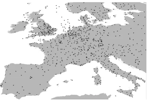
For validation purposes 6799 METereological Aerodrome Reports (METAR) from 21 points in time on the same days, obtained from a freely available online archive (Berge, 2012) were used. Geographic coordinates of the 982 European sta-tions (Fig. 1) that have published these METARs were taken from Thompson (2011).
2.3 FLS identification via SOFOS
1 km FLS masks were created from pan-sharpened chan-nels using SOFOS. SOFOS generally checks every pixel of a scene for FLS cloud properties using a range of tests (Cermak and Bendix, 2008, 2011). Most of these tests are conducted on a per-pixel basis:
Fig. 1. Positions of the METARs stations used in this study.
– cloud identification (application of a threshold derived from a histogram analysis on the difference between the 3.9 and 10.8 µm BBT);
– snow pixel elimination (application of thresholds on the 0.8 and 10.8 µm channels as well as on the Normal-ized Difference Snow Index (NDSI), which is calculated from the 0.6 and the 1.6 µm channel);
– test for liquid phase (application of a threshold of 230 K on the 10.8 µm BBT. Further tests exclude warmer ice clouds and thin cirrus clouds which are not detected by this simple threshold approach);
– test for small droplet size (application of a dynamically derived threshold on the 3.9 µm channel).
Pixels which do not pass all of these tests are rejected as obviously non-FLS. Further tests checking for spatial param-eters do not consider single pixels’ properties but properties of spatially coherent entities of cloud. For this purpose spa-tially connected pixels that were not rejected as obviously non-FLS are grouped together in entities (cf. Cermak and Bendix, 2008). The following tests are performed on these entities:
– test for stratiformity (A threshold of 2 K is applied on the standard deviation of the 10.8 µm BBT for each en-tity);
– test for low clouds (cloud top height<1000 m. The cloud top height is derived from the 10.8 µm BBT or in some cases interpolated from the height of the sur-rounding terrain).
Fig. 2. Relationship between the HRV reflectance and the re-flectance at 0.8 µm (left), and the BBT at 10.8 µm (right) for each pixel of a section of the SEVIRI scene of 17 January 2011 showing Europe.
2.4 The pan-sharpening algorithm
For global regression-based pan-sharpening as used by Bugliaro and Mayer (2004) the HRV panchromatic image is degraded to match the resolution of the SEVIRI narrow-band channels. Afterwards the pixel values of the degraded panchromatic channel can be directly related to any other SEVIRI channel as shown in Fig. 2 for a solar and a thermal channel. A regression function computed on this basis can be used to calculate approximate narrow-band spectral values from the degraded broad-band HRV channel or to calculate a high-resolution version of a given narrow-band channel from the original HRV channel as done by global regression pan-sharpening. The better the regression line fits the point cloud, the better the resulting image quality.
Obviously R2 is high (0.9008) for the displayed solar narrow-band channel but quite low (0.2491) for the thermal channel. This was to be expected, as the HRV is a solar chan-nel. This is the reason why most pan-sharpening techniques are not applicable in the thermal regions. However, local fea-tures such as the contrast between cloud and clear-sky re-gions register in both the solar and thermal rere-gions of the spectrum. The fringe area of the clouds in the northwest of the scene shown in Fig. 3 is an example of this. Here, the re-flectance in the HRV channel fades from high values in pix-els completely covered by thick clouds to low values in cloud free pixels. The pixels with a high fractional cloud cover have low BBTs in the 10.8 µm channel while pixels with less and thinner clouds have higher BBTs. Thus, a negative correla-tion can be assumed between the 10.8 µm channel and the HRV for this area. Therefore, local regressions based only on small areas of an image should be suitable for the pan-sharpening of thermal SEVIRI channels (Except SEVIRI’s water vapor channels).
A window-based pan-sharpening technique using linear local regressions is described by Hill et al. (1999). The idea of the method is not to calculate one regression function for a whole scene but one regression function for the calcula-tion of every single 3 km pixel. Each of these is based on the
Fig. 3. HRV reflectance (left) and 10.8 µm BBT (right) for a section of the SEVIRI scene from 17 January 2011 showing the Alps in the center of the image and Mediterranean Sea in the south.
Fig. 4. The pan-sharpening algorithm adapted from Hill et al. (1999). After degradation of the HRV channel (a) a regression for each 3 km pixel is calculated from the values of narrow-band pixels and degraded HRV pixels covered by a 5×5 pixels win-dow (b). Each regression is used to calculate the values for 3×3 1 km narrow-band pixels (corresponding to one 3 km pixel) from 3×3 HRV pixels (c).
degraded HRV and narrow-band pixel values in a window of 5×5 surrounding pixels. Similar to global regression pan-sharpening, a 1 km narrow-band channel is generated from the HRV channel on this basis. In contrast to global regres-sion pan-sharpening, however, not the same regresregres-sion func-tion is applied on all HRV pixels. For every HRV pixel, the regression function that was calculated for the corresponding 3 km pixel is used instead (cf. Fig. 4).
i. application of a potential regression; ii. distance weighting;
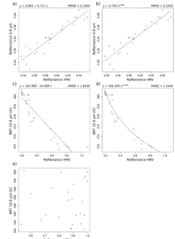
iii. different combinations of window sizes and shapes. (i) The first improvement is related to the type of regression used by the pan-sharpening algorithm. In Fig. 5 the pixel val-ues of solar and thermal channels were plotted against the degraded HRV channel for different single windows to deter-mine the nature of the relationship between these channels. Some relationships (a and b) can be described well by linear as well as potential regressions. For other windows (c and d) they can much better be described by potential regressions and in a few windows there is no relationship between both channels at all (e). The latter case is reflected in locally dete-riorated sharpening quality (see Sect. 3). The other findings suggest improving the algorithm by using a potential regres-sion in the form of
y=a×xb (1)
with
b=
n×
n
P
i=1
(ln(xi)×ln(yi))− n
P
i=1
ln(xi)× n
P
i=1
ln(yi)
n×
n
P
i=1
ln(xi)2−
n
P
i=1
ln(xi)
2 (2)
and
a=
n
P
i=1
ln(yi)−b× n
P
i=1
ln(xi)
n (3)
wherexi is the degraded HRV value and yi is the
narrow-band channel value for a window pixeli.nis the number of pixels in the current window (some windows next to an im-age’s border are cut off and therefore consist of fewer pixels). (ii) The second change to Hill et al.’s (1999) algorithm was implemented to account for Tobler’s (1970) first law of ge-ography saying that near things are more related than distant things. In this context this means that a window’s regression should particularly be affected by pixels close to the window center. Therefore we introduced a weighting factor wi for
each window pixelithat depends on the Euclidean distance di (measured in pixels) to a window’s central pixel:
wi=
( 1
di ifdi>0 1
0.5 ifdi=0
. (4)
Sincedi is 0 for the central pixel and therefore this pixel
would be weighted infinitely,di is set to 0.5 for these pixels.
To account forwi in such a way that window pixels nearer to
Fig. 5. Types of relationships between different narrow-band chan-nels and the HRV channel for single windows in a SEVIRI scene from 30 September 2003. The relationship shown in the upper row can be described well by a linear (a) and a potential regression (b). The relationship shown in the middle row is better described by a potential regression (d) than by a linear regression (c), while the re-lationship shown in (e) cannot be explained by the HRV values at all.
the window’s center have a stronger influence on the central pixel. Eqs. (2) and (3) were altered, such that:
b= n P i=1
wi× n P i=1
(ln(xi)×ln(yi)×wi)− n P i=1
(ln(xi)×wi)× n P i=1
(ln(yi)×wi) n
P i=1
wi× n P i=1
ln(xi)2×wi− n
P i=1
(ln(xi)×wi)
2 (5)
and
a=
n
P
i=1
(ln(yi)×wi)−b× n
P
i=1
(ln(xi)×wi)
n
P
i=1
wi
. (6)
of only 3×3 pixels in size, and windows of a roughly round shape were tested (round windows cannot be achieved with only a few pixels. For 3×3 pixels a cruciform shape is there-fore the nearest possible approximation to a round window. For 5×5 pixel a better approximation is possible).
Besides the use of a potential regression and the changes regarding the window shape and size, the basic idea of the pan-sharpening algorithm described by Hill et al. (1999) and shown in Fig. 4 was not altered.
2.5 Methodology of validation
Several variations of the pan-sharpening approach described in Sect. 2.4 are possible since the different window sizes and shapes, distance weighting and the two types of regression can be combined in various ways. To find the best-suited version for 1 km FLS detection, several steps of validation were necessary. First, the spectral as well as the spatial qual-ity of pan-sharpened channels were measured for each possi-ble combination (see Sect. 2.5.1). The most promising vari-ations of the pan-sharpening technique were used to sharpen SEVIRI channels for FLS masking. These masks were com-pared to reference masks and METARs (see Sect. 2.5.2). The additional METAR validation was necessary to account for some special characteristics of SOFOS regarding its reaction to an increased resolution of its input channels.
For the statistical validation of the pan-sharpened chan-nels and the comparison of FLS masks with reference masks, 144 daylight scenes under various illumination conditions from (randomly chosen) FLS appearances on 17 Novem-ber 2008, 10 DecemNovem-ber 2008, 22 DecemNovem-ber 2008 and 17 Jan-uary 2011 were utilized. For the METAR validation the num-ber of scenes was reduced to 21 to avoid overload of the used online archive.
Besides the validation using statistical measures, the qual-ity of sharpened channels and FLS masks based on them was additionally assessed visually for individual scenes. FLS masks based on channels, the resolution of which was in-creased by using a nearest-neighbour interpolation, were included in this visual validation to be able to judge to what degree differences between 3 km and 1 km channels were caused by SOFOS’ above-mentioned reaction to high-resolution input channels.
The validation study on the performance of the pan-sharpening was conducted including all seven SEVIRI chan-nels used as input for SOFOS (see Sect. 2.3).
2.5.1 Validation of pan-sharpened channels
In order to validate the spectral quality of the sharpened channels the average Root Mean Square Error (RMSE, see Strait et al., 2008) was calculated for all 144 scenes. Since it is a measure for the average difference between a data se-ries and a reference data sese-ries, it can be used for measuring the difference between the pixel values of an image and the
corresponding pixel values in a reference image. As it is in the nature of pan-sharpening that images in a resolution in which the corresponding channels did not priorly exist are created, the RMSE cannot be calculated in the SEVIRI 1 km resolution for lack of a reference image. To overcome this problem a method suggested by Thomas and Wald (2004) was utilized. According to their approach (hereinafter re-ferred to as “validation approach A”) the narrow-band chan-nels as well as the HRV channel are downsampled by the factor 3. The 3 km HRV channel obtained in this way is used to sharpen the degraded 9 km narrow-band channels. The resulting 3 km narrow-band channels can be compared to the original ones as reference. The area on the Earth’s surface covered by a window of a certain pixel size is de-pendent on the resolution of the image. As spatial aspects are taken into account by the new pan-sharpening algorithm in many ways, the validation via approach A, in which the pan-sharpening algorithm is applied on channels in a reduced resolution, may lead to wrong results regarding the window shape and size as well as the distance weighting. Therefore in a second validation approach (further referred to as “valida-tion approach B”) the narrow-band channels were sharpened to the HRV channel’s resolution and afterwards degraded to their original size, in which they were compared to the un-altered channels as reference images. Validation approach B has the disadvantage that information from individual pix-els is lost when the sharpened images are degraded to the original resolution. Thus, errors affecting only isolated pix-els cannot be accounted for by this approach. For this reason both approaches were used.
The spatial quality, a measure of the degree of similarity between the geometry of a sharpened channel and a reference image, for the different variations of the pan-sharpening al-gorithm was calculated using a slightly modified variation of a method developed by Zhou et al. (1998). By application of a Laplacian filter using the convolution mask
Dxy=
−1−1−1
−1 8 −1
−1−1−1
, (7)
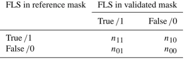
Table 1. Layout of the confusion matrices used to calculate the dif-ferent statistical measures.nis the number of occurrences.
FLS in reference mask FLS in validated mask
True/1 False/0
True/1 n11 n10
False/0 n01 n00
2.5.2 Validation of FLS masks
FLS masks based on sharpened channels were validated in two different ways. First, channels treated according to val-idation approaches A and B were used to create 3 km FLS masks via SOFOS. These masks were compared with refer-ence masks calculated by SOFOS from unaltered 3 km chan-nels. Confusion matrices (cf. Table 1) based on each pixel and each of the 144 scenes used were calculated. From these tables the following statistical measures (Wilks, 1995; Joliffe and Stephenson, 2003) were calculated (see Appendix A for formulas):
– Proportion Correct (PC);
– Bias;
– Probability of Detection (POD);
– Probability of False Detection (POFD);
– False Alarm Rate (FAR);
– Hanssen-Kuipers Discriminant (HKD);
– Additionally a new measure, the Edge Precision (EP), was developed. It describes how well the positions of edge pixels of FLS entities in the validated masks fit the positions of edge pixels of the corresponding entities in the reference mask. For this purpose the convolution maskDxywas applied on each mask and each reference
mask, in order to gain images showing only the edges of each mask’s FLS entities. For these edge images and reference edge images contingency tables were created and the POD, which in this context describes the frac-tion of edges pixels that are on the correct posifrac-tion, was calculated.
For purposes of comparison, these measures were also cal-culated for masks based on channels, the resolution of which was increased after degradation by using a simple nearest-neighbour interpolation instead of pan-sharpening. A com-parison with interpolated data was done for validation ap-proach A only since apap-proach B would gain perfect results for masks based on channels that were interpolated using a nearest-neighbour approach and degenerated afterwards.
The second approach to validate the FLS masks was nec-essary as SOFOS shows a tendency to identify different
(mostly larger) areas as FLS when the input channels’ res-olution is increased. This tendency is not caused by spec-tral errors that appear during sharpening as it can also be ob-served for channels whose resolution was increased by sim-ple nearest-neighbour interpolation (see Sect. 3). To check whether this behaviour affects the FLS masks negatively METAR data was utilized. A contingency table was calcu-lated for FLS masks based on 1 km pan-sharpened as well as on unaltered 3 km channels using the METARs as refer-ence for all scenes used. From these tables the same statis-tical measures as used for the first approach for FLS valida-tion were calculated (except the Edge Precision, as it does not make sense for the comparison with point data).
A principal problem when validating a satellite-based cloud product by making use of METAR data is mentioned by Cermak and Bendix (2007): As the instruments at ground-based stations publishing METARs are below the clouds they have another perspective on the clouds than satellites. To eliminate this problem as far as possible, not only the cloud base height but also the fractional cloud cover, the range of sight and (if included) the cloud type were uti-lized. Assuming a typical cloud thickness of 200 m for FLS (this value was empirically determined from random sam-ples taken from a cloud thickness product which was calcu-lated as described in Cermak and Bendix, 2011), METARs with cloud base heights of less than 800 m were interpreted as showing FLS presence if no cumulonimbus or cumulus congestus with a large vertical extent had been reported. Ad-ditionally, METARs reporting a line of sight of less than 1000 m were interpreted as indicating ground fog. Reports mentioning additional cloud layers above the 800 m thresh-old were interpreted as FLS-free since the additional layers would block the view from the satellite on underlying layers. Finally, METARs with a fractional cloud coverage of less than 3/8 were interpreted as free of FLS since it is very un-likely for such a low coverage that the respective pixel would be cloud-covered.
Due to the small sample size the METAR validation here should not be seen as a general validation of SOFOS’ sharp-ening quality. For a detailed METAR validation of SOFOS based on 1030 scenes see Cermak’s (2006) original work.
3 Results and discussion
3.1 The quality of sharpened channels
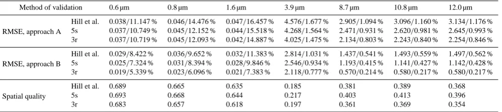
Table 2. Validation results for the spectral and spatial quality of different variations of the pan-sharpening approach. The RMSE is given in absolute values (Reflectance for solar channels, blackbody temperature for thermal channels) as well as in % of the mean pixel value of each validated scene.
Method of validation 0.6 µm 0.8 µm 1.6 µm 3.9 µm 8.7 µm 10.8 µm 12.0 µm
RMSE, approach A
Hill et al. 0.038/11.147 % 0.046/14.476 % 0.047/16.457 % 4.576/1.677 % 2.905/1.094 % 3.096/1.160 % 3.134/1.176 % 5s 0.037/10.749 % 0.045/12.152 % 0.044/15.518 % 4.268/1.564 % 2.471/0.931 % 2.620/0.981 % 2.645/0.993 % 3r 0.037/10.719 % 0.045/12.093 % 0.042/14.887 % 4.025/1.475 % 2.134/0.803 % 2.243/0.840 % 2.254/0.846 %
RMSE, approach B
Hill et al. 0.029/8.422 % 0.036/9.652 % 0.032/11.383 % 2.814/1.031 % 1.437/0.541 % 1.493/0.559 % 1.497/0.562 % 5s 0.025/7.324 % 0.031/8.394 % 0.028/9.846 % 2.546/0.934 % 1.193/0.415 % 1.141/0.427 % 1.142/0.428 % 3r 0.019/5.339 % 0.023/6.096 % 0.021/7.383 % 2.118/0.777 % 0.570/0.214 % 0.580/0.217 % 0.580/0.217 %
Spatial quality
Hill et al. 0.689 0.665 0.635 0.185 0.381 0.389 0.368
5s 0.693 0.668 0.644 0.217 0.403 0.413 0.396
3r 0.683 0.657 0.618 0.197 0.361 0.369 0.354
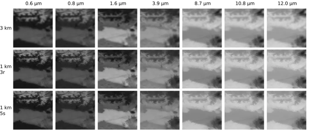
window (further referred to as 3r). The algorithm version us-ing a 5×5 pixels square window (further referred to as 5s), which yields a lower spectral quality (but is still better than that of the unaltered algorithm by Hill et al., 1999), yields the highest spatial quality. The spatial as well as the spec-tral quality of the other algorithm versions using potential regression and distance weighting (5×5 pixels round win-dow and 3×3 pixels square window, not shown in Table 2) lies between the quality of 3r and 5s. These findings are not surprising: the spectral quality improves for smaller windows consistent with the consideration that relationships between the HRV channel and the narrow-band channels are mostly spatially limited. As the sample size of each regression gets smaller for smaller windows, the regression calculated a 3 km pixels is of low significance in some cases and cannot be used for every corresponding 1 km pixel. The resulting failures occur rarely and only affect single pixels, which is why the overall spectral quality is hardly affected. Since these single pixel errors have impact on the high frequency component of an image, they strongly affect the spatial quality. Due to the trade-off between the spatial and the spectral quality the window size and shape has to be chosen depending on the intended use. In order to check whether the spatial or spec-tral quality of SOFOS input channels is more important for the quality of the FLS detection, the validation of the result-ing masks was necessary to choose the best version of the pan-sharpening algorithm.
Figure 6 shows the quality of the new algorithm using 5s and 3r for the sharpening of each of the SOFOS input chan-nels. For the 3r version the mentioned errors in individual pixels can be clearly identified. Since the lowered spectral quality of the 5s variation cannot be recognized by the hu-man eye, a 5×5 pixels window seems to be a suitable choice for visualization purposes. The scene shows fog in the Po Valley in the center and the snow-covered Alps in the north. North of the fog in the plain Lake Iseo can be recognized. For each channel these different surfaces were sharpened well. The fog margin is very sharp and even small valleys, along which the fog reaches into the northern parts of the Apen-nine Mountains, can be recognized. In the southeast of the
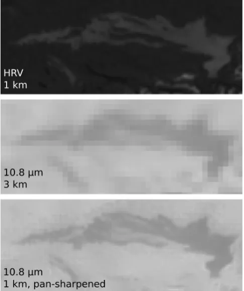
scene there are high clouds above the FLS, which are shown in dark shades in the thermal channels (low temperature). In the thermal spectrum the spatial quality of the scene is low-ered for these clouds by some weakly pronounced rectangu-lar artifacts in the original 3 km resolution. These artifacts are caused by a situation as shown in Fig. 5e. As no relationship between the narrow-band channel and the degraded HRV channel can be established, a more or less horizontal regres-sion function is assumed, which is why for these areas quite similar values are assigned to all 1 km pixels covered by the same 3 km pixel. These flaws do not affect the spectral qual-ity. Further they are rare and can mostly be observed for high clouds, especially for cumuliform clouds where the bright-ness of the HRV channel is strongly influenced by the illu-mination geometry. Therefore they should only minimally affect the quality of FLS masks based on sharpened chan-nels. In addition to Fig. 6, the pan-sharpening quality of 5s is demonstrated for a thermal channel in Fig. 7 showing an FLS entity covering Lake Constance and adjacent valleys. 3.2 The quality of FLS masks based on sharpened
channels
Fig. 6. Sharpening results for different variations of the pan-sharpening algorithm and each of SOFOS’ input channels showing fog in the Po Valley on 22 December 2008. In order to achieve better comparability the 3 km channels were interpolated to the size of the 1 km images via nearest-neighbour interpolation.
Table 3. Statistical measures describing the quality of FLS masks based on channels that were sharpened by different variations of the pan-sharpening algorithm as well as on interpolated channels.
Method of validation PC Bias POD POFD FAR HKD EP
Validation approach A
Hill et al. 0.933 0.987 0.746 0.038 0.244 0.708 0.336
5s 0.936 1.045 0.787 0.040 0.246 0.747 0.356
3r 0.950 1.0002 0.816 0.029 0.184 0.787 0.425
Interpolation 0.948 1.001 0.807 0.030 0.194 0.777 0.372
Validation approach B
Hill et al. 0.956 1.011 0.842 0.026 0.167 0.816 0.502
5s 0.966 1.013 0.880 0.021 0.132 0.859 0.612
3r 0.974 1.002 0.904 0.015 0.098 0.888 0.703
Best Possible Result 1 1 1 0 0 1 1
same can be observed for the bias, the POD, the POFD, the FAR and the HKD. Although Figs. 6 and 7 show that the spatial quality of the 5s method is much higher than that of a simple interpolation, even the Edge Precision (EP) of sharp-ened masks is lower than that of masks based on interpolated channels. All of these findings are most probably caused by an insufficient spectral quality of the original algorithm and the 5s version. This hypothesis is supported by the fact that only the 3r variation, which has the best spectral quality, out-performs the interpolation for all statistical measures. In ad-dition this variant delivers a spatial quality (cf. Fig. 6) that is much higher than that of a simple interpolation and thus gains the best Edge Precision. Therefore it is the best choice for the sharpening of SOFOS input channels.
3.3 Comparison of 3 km and 1 km FLS masks
Fig. 7. Fog covering Lake Constance and adjacent valleys on 17 Jan-uary 2011. In order to achieve better comparability the 3 km chan-nel was interpolated to the size of the 1 km images via nearest-neighbour interpolation.
Table 4. Results of the METAR validation.
Statistical 3 km 1 km measure masks masks
PC 0.574 0.600
Bias 0.197 0.378
POD 0.654 0.658
POFD 0.057 0.107
FAR 0.346 0.342
HKD 0.072 0.141
is enhanced, the degree of underestimation was lowered and the changes in the degree of overestimation depend on the measure for overestimation, FLS masks do, all in all, benefit from SOFOS’ reaction to resolution enhancement.
Additional insights into the degree of enhancement of FLS masks via pan-sharpening can be obtained from Figs. 8 to 12. Figure 8 shows fog on 17 January 2011 covering Lake Con-stance in the northeast and Lake Geneva and Lake Neuchˆatel in the southwest. The outlines of FLS masks based on 3 km SEVIRI channels as well as on channels that where sharp-ened by the 3r method are shown. In both resolutions the FLS has been detected very well. Nevertheless, the quality of the
Fig. 8. 3 km (top) and 1 km (middle) FLS mask for fog in Southern Germany and Switzerland on 17 January 2011. White line=boundary of the masks. White arrow=detail that strongly benefits from the resolution enhancement.
1 km mask is much higher, since fine details that cannot be displayed at the 3 km resolution can be found along the bor-ders of the FLS entities. For example the fog-covered Thur Valley (white arrow) south of Lake Constance can hardly be recognized in the 3 km resolution, while its shape can be identified precisely in the 1 km mask. Figure 9 shows a fog occurrence on the same date in central Germany. Again, many details (white arrows), especially fog that is restricted in its extent by the shape of valleys can only be recognized in the 1 km resolution. In addition, the tendency of SOFOS to identify different areas as FLS for 1 km input channels had a large impact on the quality of the 1 km FLS mask. The western FLS entity is hardly covered by the 3 km FLS mask, while it was well-detected from pan-sharpened as well as in-terpolated (black outline) 1 km channels.
Fig. 9. 3 km (top) and 1 km (center) FLS mask for fog in Cen-tral Germany on 17 January 2011. White line=boundary of the 3 km and 1 km masks. Black line=boundary of an additional FLS mask based on channels interpolated to 1 km resolution (Notice that this mask matches the 3 km mask perfectly for the eastern FLS entity, which is why the black outline is not visible here). White arrows=details that strongly benefit from the resolution enhance-ment.
masks and the DEM shows that many terrain features affect-ing the shape of the fog entity (white arrows) like many small valleys in the northern Apennines, the Superga hill range ris-ing from the middle of the fog or the remnants of a moraine arc in the northwest of the scene, are hardly reflected in the 3 km mask. In the 1 km mask, all of these features can be dis-tinguished easily. In addition, the 3 km mask does not cover the western part of the fog, while the 1 km mask does. A drawback of the sharpened mask is marked by a black ar-row. A hole in the mask, where the FLS was not recognized, can be found here. Again, these differences to the 3 km mask were not caused by a low quality of the sharpening but by the effect of the increased resolution of its input channels on SOFOS. For interpolated input channels (black outline) the hole in the mask is even bigger.
Fig. 10. FLS masks (indicated by the white outline) in 3 km (left) and 1 km (center) resolution for fog in the Po Valley on 22 De-cember 2008. The masks’ outlines are underlaid by a DEM. White line=boundary of the 3 km and 1 km masks. Black line=boundary of an additional FLS mask based on channels interpolated to 1 km resolution. White arrows=details that strongly benefit from the res-olution enhancement. Black Arrow=area where FLS was not de-tected.
Figure 11 shows FLS in Southern Germany delimited by the northern margin of the Alps. Again, the topography-induced shape of the FLS, including many valleys (white ar-rows), can be much better identified in the 1 km mask than in the 3 km mask. There are also some areas where FLS could only be identified on the basis of the 1 km channels (dark-grey arrow) or on the basis of the 3 km channels (light-(dark-grey arrow). A comparison of the 1 km mask with a mask based on interpolated channels (black outline) shows that these differ-ences are, again, caused by the reaction of SOFOS to high-resolution input channels, which has (as the METAR valida-tion has shown) a positive overall influence.
Snow close to fog areas in Figs. 8, 10 and 11 was not misidentified as FLS in any case, which is a big advantage of the new method over a threshold approach. However, if fog and snow or other clouds are situated directly side by side, they fall into common windows and therefore the algorithm tries to describe the dependency of a narrow-band channel from the pan channel by the same regressions for both mate-rials. Since this is not reasonable in many cases, a situation similar to that shown in Fig. 5e could occur and therefore drawbacks in the spatial quality of the sharpened channels and in the resulting mask should be possible. 3 km artifacts in the 1 km FLS mask caused by this could not be observed for the margins of snow-covered areas or for any entity of ground fog. In the margin area of FLS without ground con-tact, however, this kind of artifacts could be observed in rare cases (cf. Fig. 12).
Fig. 11. 3 km (top) and 1 km (center) FLS masks (indicated by the white outline) for fog north of the Alps on 2 February 2011. The masks’ outlines are underlaid by a DEM. White line=boundary of the 3 km and 1 km masks. Black line=boundary of an additional FLS mask based on channels interpolated to 1 km resolution. White arrows=details that strongly benefit from the resolution enhance-ment. Black arrows=Areas that were not identified as FLS regard-less of the resolution. Light grey arrow=an area that was only de-tected as FLS in 3 km resolution. Dark grey arrow=an area that was only detected as FLS in 1 km resolution.
4 Conclusion and outlook
A method for the creation of 1 km fog and low stratus (FLS) masks from MSG SEVIRI data was presented. The new method uses an innovative application for a further devel-oped version of an existing pan-sharpening algorithm suit-able to enhance the spatial quality of solar as well as ther-mal 3 km SEVIRI channels to 1 km by using the instru-ment’s panchromatic HRV channel. The resulting 1 km syn-thetic narrow-band channels are used as input for the well-validated FLS detection scheme SOFOS in order to produce 1 km FLS masks. The pan-sharpening approach strongly im-proves the spatial quality of the resulting masks. As the shape of many small valleys cannot be distinguished at a 3 km
Fig. 12. FLS masks (indicated by the white outline) for low stratus without ground contact over Central France on 10 December 2008 based on 3 km (left) and 1 km (right) SEVIRI channels. The spatial quality of the 1 km mask is reduced by rectangular artifacts in the 3 km resolution.
spatial resolution, this is especially important for the proper mapping of FLS entities delimited by topography. The new approach combines a relatively high spatial resolution with the high temporal resolution of a geostationary instrument. Therefore it offers new possibilities for short-range forecast-ing and the creation of fog climatologies. Errors in the high-resolution FLS masks caused by a low spectral quality of the sharpened input channels could not be found. The only flaws which can be traced back to the pan-sharpening algorithm are local reductions of the spatial quality reflected in rectangular artifacts in the mask border. These artifacts are rare and could only be observed for the fuzzy border of FLS without ground contact. As they never reduce the spatial quality of the mask to a level lower than that of 3 km masks, a sharpening of SOFOS input channels using the improved pan-sharpening algorithm seems to be a suitable method to gain high quality 1 km FLS masks.
Appendix A
Formulas utilized for the validation of FLS masks
The following formulas were used for calculating of the sta-tistical measure used in Sect. 2.5.2:
PC= n11+n00
n11+n10+n01+n00
(A1) Bias=n11+n01
n11+n10
(A2) POD= n11
n11+n10
(A3) POFD= n01
n01+n00
(A4) FAR= n01
n11+n01
(A5)
HKD=POD−POFD (A6)
Acknowledgements. This research was funded by a grant from the
German Research Council DFG (BE 1780/14-1).
Edited by: A. Kokhanovsky
References
Bendix, J. and Bachmann, M.: A method for detection of fog us-ing AVHRR imagery of NOAA satellites suitable for operational purposes, Meteor. Rundsch., 43, 169–178, 1991 (in German). Bendix, J., Thies, B., and Cermak, J.: A feasibility study of daytime
fog and low stratus detection with TERRA/AQUA-MODIS over land, J. Appl. Meteorol., 13, 111–125, 2006.
Bensi, P., Aminou, D., Bezy, J. L., Stuhlmann, R., Rodriguez, A., and Tjemkes, S.: Overview of meteosat third generation (MTG) activities, Second MSG RAO Workshop, 9–10 September 2004, Salzburg, Austria, 2004.
Berge, D.: Navlost.eu – Navigation and Positioning Resources, available at: http://www.navlost.eu (last access: 20 March 2012), 2012.
Bugliaro, L. and Mayer, B.: Study on quantitative use of the High Resolution Visible channel onboard the Meteosat Second Gener-ation satellite, final report phase II, Technical Report, EUMET-SAT, Darmstadt, Germany, 2004.
Cermak, J.: SOFOS – A new Satellite-based Operational Fog Obser-vation Scheme, PhD thesis, Philipps-University Marburg, 2006. Cermak, J. and Bendix, J.: Dynamical nighttime fog/low stratus
de-tection based on Meteosat SEVIRI data: A feasibility study, Pure Appl. Geophys., 164, 1179–1192, 2007.
Cermak, J. and Bendix, J.: A novel approach to fog/low stratus de-tection using Meteosat 8 data, Atmos. Res., 87, 279–292, 2008.
Cermak, J. and Bendix, J.: Detecting ground fog from space – a microphysics-based approach, Int. J. Remote Sens., 32, 3345– 3371, 2011.
Cermak, J., Bendix, J., and Dobbermann, M.: FMet – an integrated framework for data processing for operational scientific applica-tions, Comput. Geosci., 34, 1638–1644, 2008.
Deneke, H. M. and Roebeling, R. A.: Downscaling of METEOSAT SEVIRI 0.6 and 0.8 µm channel radiances utilizing the high-resolution visible channel, Atmos. Chem. Phys., 10, 9761–9772, doi:10.5194/acp-10-9761-2010, 2010.
EUMETSAT: EUMETCast, available at: http://www.eumetsat.int/ Home/Main/DataAccess/EUMETCast/index.htm (last access: 20 March 2012), 2012.
Eyre, J. R., Brownscombe, J. L., and Allam, R. J.: Detection of fog at night using Advanced Very High Resolution Radiometer (AVHRR) imagery, Metereol. Mag., 113, 265–271, 1984. Gultepe, I., Tardif, R., Michaelides, S. C., Cermak, J., Bott, A.,
Bendix, J., M¨uller, M. D., Pagowski, M., Hansen, B., Ellrod, G., Jacobs, W., Toth, G., and Cober, S. G.: Fog Research: A Review of Past Achievements and Future Perspectives, Pure Appl. Geo-phys., 164, 1121–1159, 2007.
Hill, J., Diemer, C., St¨over, O., and Udelhoven, T.: A local corre-lation approach for the fusion of remote sensing data with spa-tial resolutions in forestry applications, Int. Arch. Photogramm. Remote Sens., 32, Part 7-4-3 W6, Valladolid, Spain, 3–4 June, 1999.
Joliffe, I. T. and Stephenson, D. B.: Forecast Verification – A Prac-titioner’s Guide in Atmospheric Science, John Wiley & Sons, Chicester, West Sussex, UK, 2003.
Kudoh, J. and Noguchi, S.: Identification of fog with NOAA AVHRR images, IEEE T. Geosci. Remote Sens., 29, 704–709, 1991.
Lee, T. F., Turk, F. J., and Richardson, K.: Stratus and fog products using GOES-8-9 3.9-µm data, Weather Forecast., 12, 664–677, 1997.
Liu, D. and Pu, R.: Downscaling thermal infrared radiance for sub-pixel land surface temperature retrieval, Sensors, 8, 2695–2706, 2008.
Strait, M., Rahmani, S., and Markujev, D.: Evaluation of pan-sharpening methods, Technical Report, UCLA Department of Mathematics, Los Angeles, 2008.
Thomas, C. and Wald, L.: Assessment of the quality of fused prod-ucts, Proceedings of the 24th EARSeL Symposium “New Strate-gies for European Remote Sensing”, Dubrovnik, 1–25, 2004. Thompson, G.: Untitled list of ICAO airport codes, available
at: http://www.rap.ucar.edu/weather/surface/stations.txt (last ac-cess: 22 May 2011), 2011.
Tobler, W.: A computer movie simulating urban growth in the De-troit region, Econ. Geogr., 46, 234–240, 1970.
USGS: GTOPO30, available at: http://eros.usgs.gov/#/Find Data/ Products and Data Available/gtopo30 info (last access: 22 May 2011), 1996.
Wilks, D. S.: Statistical Methods in the Atmospheric Sciences – An Introduction, Academic Press, San Diego, 1995.