www.the-cryosphere.net/8/1347/2014/ doi:10.5194/tc-8-1347-2014
© Author(s) 2014. CC Attribution 3.0 License.
Modelling the evolution of the Antarctic ice sheet since the last
interglacial
M. N. A. Maris1, B. de Boer1,2, S. R. M. Ligtenberg1, M. Crucifix3, W. J. van de Berg1, and J. Oerlemans1 1Institute for Marine and Atmospheric Research Utrecht, Utrecht University, P.O. Box 80005, 3508 TA Utrecht, the Netherlands
2Department of Earth Sciences, Faculty of Geosciences, Utrecht University, Utrecht, the Netherlands
3Earth and Life Institute (ELI), Georges Lemaître Centre for Earth and Climate Research (TECLIM), Place Louis Pasteur 3, SC10 – L4.03.08, 1348 Louvain-la-Neuve, Belgium
Correspondence to: M. N. A. Maris ([email protected])
Received: 4 December 2013 – Published in The Cryosphere Discuss.: 6 January 2014 Revised: 21 June 2014 – Accepted: 24 June 2014 – Published: 30 July 2014
Abstract. We present the effects of changing two slid-ing parameters, a deformational velocity parameter and two bedrock deflection parameters on the evolution of the Antarc-tic ice sheet over the period from the last interglacial until the present. These sensitivity experiments have been conducted by running the dynamic ice model ANICE forward in time. The temporal climatological forcing is established by inter-polating between two temporal climate states created with a regional climate model. The interpolation is done in such a way that both temperature and surface mass balance follow the European Project for Ice Coring in Antarctica (EPICA) Dome C ice-core proxy record for temperature. We have de-termined an optimal set of parameter values, for which a real-istic grounding-line retreat history and present-day ice sheet can be simulated; the simulation with this set of parameter values is defined as the reference simulation. An increase of sliding with respect to this reference simulation leads to a decrease of the Antarctic ice volume due to enhanced ice ve-locities on mainly the West Antarctic ice sheet. The effect of changing the deformational velocity parameter mainly yields a change in east Antarctic ice volume. Furthermore, we have found a minimum in the Antarctic ice volume during the mid-Holocene, in accordance with observations. This is a robust feature in our model results, where the strength and the tim-ing of this minimum are both dependent on the investigated parameters. More sliding and a slower responding bedrock lead to a stronger minimum which emerges at an earlier time. From the model results, we conclude that the Antarctic ice sheet has contributed 10.7±1.3 m of eustatic sea level to the
global ocean from the last glacial maximum (about 16 ka for the Antarctic ice sheet) until the present.
1 Introduction
to have the same climate as the PD. An interpolation method is used to create a climatological forcing that is continuous in time, making use of the EPICA Dome C ice core record (Jouzel et al., 2007). This method leads to a realistic simula-tion of the climate while still being computasimula-tionally feasible. The interpolation method is described in detail in Sect. 2.2.
Despite numerous studies on the subject, little is known about the sediment beneath the AIS and its effects on the magnitude and variations in sliding. Consequently, the ef-fects of sediment on sliding is heavily parameterised in dy-namic ice models (e.g. Bueler and Brown, 2009; Pollard and DeConto, 2012a). Furthermore, dynamic ice models gener-ally make use of Glen’s isotropic flow law (Glen, 1958), while ice is a highly anisotropic material. Therefore, so-called enhancement factors are introduced (see for instance Huybrechts, 1992; Ma et al., 2010; De Boer, 2012; Pol-lard and DeConto, 2012b). These factors are different for grounded ice (which can be described by the shallow ice ap-proximation, the SIA) and sliding or floating ice (both de-scribed by the shallow shelf approximation, the SSA). Ad-ditionally, the lithosphere is thinner under the West Antarc-tic ice sheet (WAIS) than under the East AntarcAntarc-tic ice sheet (EAIS) (Huerta and Harry, 2007). However, little is known about the lithospheric structure under Antarctica and how it influences the ice sheet (Morelli and Danesi, 2004). A thin-ner lithosphere is associated with smaller response times of the bed elevation to the ice load and to less rigidity, that is, the amplitude of the deflection is larger for a given ice load (Le Meur and Huybrechts, 1996).
In this study we use the dynamical ice-sheet model ANICE (De Boer et al., 2012) to investigate how the AIS reacts to different lithospheric and sliding parameters by doing sensi-tivity experiments on the period of 120 ka to the present. The last interglacial period ended around 120 ka, when tempera-tures and sea levels were close to PD values. The goal of this study is to learn how sensitive the AIS is to changes in differ-ent model parameters. Additionally, we want to find an opti-mal set of parameter values for which a realistic grounding-line retreat history and PD ice sheet are simulated. With these parameter values, a more focussed study on the behaviour of the AIS during the last deglaciation can be facilitated.
2 Methods
Starting with an initial state of the AIS 120 ka, see Sect. 2.1, the dynamic ice model ANICE has been run forward to the present. The applied climatological forcing combines the output of a regional atmospheric climate model with the EPICA Dome C ice core record and will be discussed in Sect. 2.2. The surface mass balance is part of this climato-logical forcing, whereas the basal mass balance is deduced from the basal heat flux where the ice is grounded, and from the ocean heat flux (see Sect. 2.3) where ice is in contact with water. Calving is parameterised by removing all
float-ing ice below a threshold thickness of 250 m, at the end of every period of 300 yr. Other values for these two calving parameters have been tested as well, where the threshold thickness has been varied between 100 and 300 m and the period between 100 and 500 yr. These parameterisations did not change the grounding line or the grounded ice volume significantly, and therefore we decided to use the original pa-rameterisation with a threshold ice thickness of 250 m and a calving period of 300 yr.
Ice velocities are calculated in ANICE by using both the SIA and the SSA (Bueler and Brown, 2009). The SIA is used as a basis for the velocities on the grounded part of the ice sheet and the SSA is used for ice-shelf and sliding velocities. The SSA velocity, which is assumed to be the basal veloc-ity, and the SIA velocity are superposed as in the Potsdam Parallel Ice Sheet Model (PISM-PIK) (Winkelmann et al., 2011). Both approximations include an enhancement factor because, generally, the SIA underestimates the ice velocity and the SSA overestimates it (Ma et al., 2010). We varied both enhancement factors in the sensitivity experiments.
Whether the ice is sliding or not and how fast it is sliding also depends on the sediments underneath the ice. Almost nothing is known about the material which these sediments consist of, but the assumption is that the subglacial sediments (till) are weaker when the bed is beneath sea level. Below sea level the bed is assumed to have a marine history, leading to a smaller grain size and clay-like till with little pore space. Therefore, water stays mostly on top of the till, enhancing the sliding potential of the ice (Clarke, 2005). The weakness of the till has been varied in the sensitivity experiments as well.
In addition to the enhancement factors and the till, there is another factor influencing the evolution of the AIS: the thickness of the lithosphere. In ANICE, an ELRA (Elastic Lithosphere, Relaxed Asthenosphere) model is included to describe the response of the bed elevation to the ice loading history (Le Meur and Huybrechts, 1996). The bed underneath the ice sheet is described as a thin, elastic lithosphere, con-trolling the geometric shape of a deformation; the elasticity is determined by the flexural rigidity in the model. The litho-sphere floats on a viscous asthenolitho-sphere, which governs the time-dependent characteristics of a deformation. In the sensi-tivity experiments, the response time and the flexural rigidity of the bedrock have been varied. The theory behind the sen-sitivity experiments will be discussed in Sect. 2.4.
2.1 Initial state
Figure 1. The PD surface elevation, used as an initial configuration
120 ka. The white line indicates the grounding line and the black line separates the WAIS from the EAIS. The light blue box shows the ANICE model domain.
between the EAIS and the WAIS. This line is drawn at 30◦W→86◦S→160◦E. The model ANICE is run forward in time with the PD surface temperatures and a fixed geome-try (the ice thickness is kept fixed), such that the 3-D temper-ature field within the ice reaches a thermodynamical equi-librium. The output of this simulation has been used as the initial state.
2.2 Climatological forcing
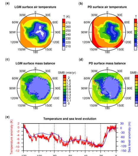
We use the PD climate as an initial forcing at 120 ka and a simulation of the LGM climate at the LGM. The climato-logical forcing of ANICE consists of the 2 m air temperature and the surface mass balance (SMB). The two climate states (PD and LGM) are a product of the regional atmospheric climate model RACMO2. This model includes a sophisti-cated snow model (Ettema et al., 2009) and albedo scheme (Kuipers Munneke et al., 2011) in order to realistically sim-ulate snow–air interactions and liquid water processes (melt, percolation, retention, refreezing and runoff). In combination with a better horizontal grid resolution (55 km), RACMO2 is therefore able to simulate a more realistic Antarctic cli-mate than a general circulation model (GCM) (Ligtenberg et al., 2013). When forced with re-analysis data for the recent past, RACMO2 has yielded realistic results over Antarctica, compared to in situ observations (Van de Berg et al., 2006; Lenaerts et al., 2012).
For the simulation of the Antarctic LGM climate, RACMO2 is forced with a GCM simulation from the Hadley Centre Coupled Model, version 3 (HadCM3). The HadCM3 model was chosen because it consistently performs among the better GCMs above the Antarctic region (Maris et al., 2012). The method of laterally forcing RACMO2 with GCM data was previously successfully used in future scenario sim-ulations for the AIS (Ligtenberg et al., 2013). RACMO2 is forced at the lateral boundaries of the domain with fields of
( ) ( )
( ) ( )
( )
Figure 2. RACMO2 output fields of (a) the LGM temperature, (b) the PD temperature, (c) the LGM surface mass balance in metres
ice equivalent per year and (d) the PD surface mass balance. Panel
(e) – the temperature evolution according to the EPICA Dome C ice
core (Jouzel et al., 2007) is shown in red and the sea level evolution according to Bintanja and van de Wal (2008) in blue.
temperature, wind components, surface pressure and specific humidity from the GCM simulation. Every six hours, the model value is linearly interpolated with the external forcing. Sea-ice concentration and sea-surface temperature are also prescribed by HadCM3. The extent and surface height of the AIS are part of the RACMO2 input as well, but these vari-ables are not well known for the LGM. We used the ICE-5G reconstruction by Peltier (2004) to provide RACMO2 with topographical data because this topography was also used to produce the HadCM3 data. For the PD, ALBMAP data pro-vided the topography, see Fig. 1. The output of RACMO2 has been integrated over 25 years to yield a representative climate for the LGM and PD periods.
We use this interpolation method instead of a simple ice-core based interpolation of the temperature and SMB fields because the patterns should evolve with the topography of the ice sheet. As the topography of the ice sheet lags behind the air temperature, evolving the patterns with air temperature in-stead of linearly in time would change them too quickly. The changing climate (temperature and SMB) between 120 ka, the LGM and the PD is derived from the two RACMO2 cli-mate states by a linear interpolation technique in three steps, which is done for each spatial point (i, j):
1. Normalisation of the data (division by the mean) to de-termine the temperature and SMB patterns:
Tnorm(i, j,LGM)=
T (i, j,LGM) Tmean(LGM)
, (1)
Tnorm(i, j,PD)=
T (i, j,PD) Tmean(PD)
. (2)
Here, T is the temperature (in K), and the means are taken over the continent. The same equations hold for the SMB (in m i.e. yr−1, where i.e. is ice equivalent). 2. Linear interpolation through time from one normalised
state to the next. In the normalised data, only the spa-tial patterns are visible (e.g. it is colder in the interior of the ice sheet than near the coast). With the interpolation those patterns are evolved through time. For tempera-ture from the last interglacial (the reference (ref), where the temperature is the same as the PD temperature) to the LGM:
Tnorm(i, j, t )=
1− t−tref
tLGM−tref
·Tnorm(i, j,PD) + t−tref
tLGM−tref
·Tnorm(i, j,LGM) (3) For temperature from the LGM to the present, where
tPD=0: Tnorm(i, j, t )=
1−t−tLGM −tLGM
·Tnorm(i, j,LGM) + t−tLGM
−tLGM
·Tnorm(i, Tnorm)(i, j,PD) (4)
Again, the same equations are applied to the SMB. 3. Multiplication by a factor in such a way that the original
states remain the same. For temperature:
T (i, j, t )=Tnorm(i, j, t )·(Tmean(PD)+fT·1T ) (5) And for the SMB (in metres ice equivalent per year): SMB(i, j, t )=SMBnorm(i, j, t )·(SMBmean(PD)
+fSMB·1T ) (6)
Here,1T is the temperature anomaly as given by the EDC (EPICA Dome C) ice core record from Jouzel et al. (2007). The multiplication factors before1T are chosen in such a way that multiplying them with1T, gives the difference be-tween the LGM and PD mean values. That is,
fT =
Tmean(LGM)−Tmean(PD)
1T (LGM) . (7)
The temperature anomaly 21 ka was−9.2 K according to the EDC record. Filling this in for1T (LGM), and subtract-ing the mean PD temperature of 254.8 K from the LGM mean temperature of 247.9 K, this gives a value forfT of 0.75. The mean SMB at the LGM is 0.12 m i.e. yr−1and presently it is 0.21 m i.e. yr−1, so using
fSMB=
SMBmean(LGM)−SMBmean(PD)
1T (LGM) , (8)
gives a value forfSMBof 0.0098. 2.3 Oceanic forcing
The basal mass balance (BMB) of floating ice is determined by the influence of the ocean water on the ice following Hol-land and Jenkins (1999):
BMB=Fmelt·ρo·cpo·γT ·(To−Tf) / (L·ρi) . (9)
The BMB depends on the difference between the water tem-perature (To) and the freezing temperature (Tf). A more de-tailed list of model parameters and variables, and the symbols used to represent them in this paper, is given in Table 1. The ocean temperature is given by
To=(θo−1.7)+0.3·1T −0.12·10−310−3·Dshelf. (10) The PD ocean potential temperature (θo), is provided by ECHAM53, from the Paleoclimate Modelling Intercompar-ison Project Phase II (PMIP2) (Braconnot et al., 2007). A cross-section of θo at 300 m depth is shown in Fig. 3. ECHAM53 was chosen because both the vertical and hor-izontal patterns match observations from the World Ocean Circulation Experiment (WOCE) atlas (Orsi and Whitworth III, 2004). However,θois on average too high by about 1.7◦, so this value is subtracted from theθo-field. Furthermore, the coarse resolution (which is already higher in ECHAM53 than in most other GCMs) precludes the output of beneath the in-nermost ice shelves. Therefore, the data have been interpo-lated for these regions by simple inverse distance interpola-tion. The temperature anomaly with respect to the present (1T) is retrieved from the EDC ice core record, see Fig. 2e. Furthermore, to go from potential temperature to real tem-perature, a lapse rate is included, multiplied by the depth of the ice shelf (Dshelf). The mean lapse rate in water is 0.12×10⁻³K m−1(Knauss, 1997) and the freezing temper-ature is given by
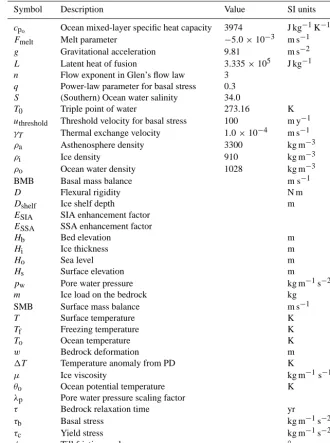
Table 1. List of used symbols, their descriptions and values and SI units when applicable.
Symbol Description Value SI units
cpo Ocean mixed-layer specific heat capacity 3974 J kg
−1K−1
Fmelt Melt parameter −5.0×10⁻³ m s−1 g Gravitational acceleration 9.81 m s−2
L Latent heat of fusion 3.335×10⁵ J kg−1
n Flow exponent in Glen’s flow law 3
q Power-law parameter for basal stress 0.3
S (Southern) Ocean water salinity 34.0
T0 Triple point of water 273.16 K uthreshold Threshold velocity for basal stress 100 m y−1 γT Thermal exchange velocity 1.0×10⁻⁴ m s−1
ρa Asthenosphere density 3300 kg m−3 ρi Ice density 910 kg m−3 ρo Ocean water density 1028 kg m−3
BMB Basal mass balance m s−1
D Flexural rigidity N m
Dshelf Ice shelf depth m
ESIA SIA enhancement factor ESSA SSA enhancement factor
Hb Bed elevation m
Hi Ice thickness m
Ho Sea level m
Hs Surface elevation m
pw Pore water pressure kg m−1s−2 m Ice load on the bedrock kg
SMB Surface mass balance m s−1
T Surface temperature K
Tf Freezing temperature K
To Ocean temperature K
w Bedrock deformation m
1T Temperature anomaly from PD K
µ Ice viscosity kg m−1s−1
θo Ocean potential temperature K λp Pore water pressure scaling factor
τ Bedrock relaxation time yr
τb Basal stress kg m−1s−2 τc Yield stress kg m−1s−2
φ Till friction angle ◦
The height of the sea level changes with time and plays a key role in the evolution of the AIS (Pol-lard and DeConto, 2009; De Boer et al., 2012). In this study, the sea-level anomaly is taken from work by Bintanja and van de Wal (2008). They used an ice-sheet model in combination with an ocean-temperature model to extract a 3 Myr record of air temperature and sea level from benthic oxygen isotopes. The part of the record that is used in this study is presented in Fig. 2e. We used this record because it is representative of eustatic sea-level change.
2.4 Varied parameters in the sensitivity experiments 2.4.1 Ice-flow enhancement factors
As mentioned before, the SIA and SSA velocities in ANICE are superposed to calculate the ice velocity. The SIA velocity is given by
VSIA= −2(ρi·g)n· |∇Hs|n−1·
∇Hs z Z
b
ESIA·A(T∗)·(Hs−z)ndζ, (12)
Figure 3. Ocean potential temperature at 300 m depth, as given by
ECHAM53 (Braconnot et al., 2007). In the areas where no water is present, a mask has been placed (transparent areas in the figure).
flow-rate factor (A(T∗)) depends on the temperature, which is corrected for pressure melting. The SIA enhancement fac-tor (ESIA) is varied between 7 and 11 in the sensitivity exper-iments. This factor determines how much the deformational flow of the ice is enhanced. There is also an SSA enhance-ment factor,ESSA, which appears in the vertically averaged viscosityµ:
µ= 1
2(ESSA·A)1/n · " ∂u ∂x 2 + ∂v ∂y 2 +∂u ∂x ∂v ∂y+ 1 4 ∂u ∂y+ ∂v ∂x
2#12−nn , (13)
in the SSA velocity equations:
∂ ∂x
2µHi
2∂u ∂x+ ∂v ∂y + ∂ ∂y µHi ∂u ∂y+ ∂v ∂x
+τb,x=ρigHi ∂Hs
∂x , (14)
and
∂ ∂y
2µHi
2∂v ∂y+ ∂u ∂x + ∂ ∂x µHi ∂v ∂x+ ∂u ∂y
+τb,y=ρigHi ∂Hs
∂y . (15)
In Eq. (13),Ais the vertical mean ofA(T∗),uandv are the SSA velocities in thexandy direction respectively, and
τb,x andτb,y are the basal shear stresses in thex andy di-rection.ESSA is varied between 0.6 and 1.0. The variations of both enhancement factors for the sensitivity experiments have been established following the work of Ma et al. (2010). They suggest that the SIA enhancement factor should lie be-tween 5 and 6, and the SSA enhancement factor should lie between 0.5 and 0.7 for ice shelves and between 0.6 and 1 for ice streams. As ANICE uses the same enhancement fac-tor for ice streams and ice shelves,ESSAhas been chosen in
the range of the ice streams as these are the most important for the evolution of the AIS over time. AnESIA of 5 or 6 would yield too much ice on the EAIS, therefore a range of higher values has been chosen for this parameter, see Sect. 4. 2.4.2 Basal stress
In ANICE, the basal stress (τbin Eqs. 14–15) is determined as a function of the yield stress and the basal sliding velocity, as in Bueler and Brown (2009). The basal stress is given by
τb=τc· V
q−1 SSA
uqthreshold·, (16)
whereτcis the yield stress:
τc=(tanφ)·(ρigHi−pw) , (17) andpwis the pore water pressure:
pw=0.96·λp·ρi·g·Hi. (18) Here,λpis a scaling factor such that the pore water pressure is maximal when the ice is resting on bedrock at or below sea level. Below sea level, the pores in the till are assumed to be saturated with water soλpis then equal to 1. The factorλp is scaled with the height above sea level up until 1000 m. At and above 1000 m,λpis equal to 0. Finally, the till friction angle in Eq. (17) (φ) is parameterised by
φ=
φmin ifHb≤ −103,
−Hb 103·φmin+
1+Hb
103
·φmax if −103< Hb<0,
φmax if 0< Hb.
(19)
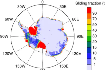
φmaxis kept constant at a value of 30◦in the sensitivity ex-periments andφminis varied between 8◦and 12◦.φmin deter-mines the sliding below−1000 m and partly between−1000 and 0 m, and therefore controls the sliding on large parts of the WAIS. The assumption here is that the till is weaker when situated below sea level and therefore the friction angle is smaller, and sliding more dominant. This effect can clearly be seen in Fig. 4, where the fraction of sliding velocity with respect to the total ice velocity is shown for the reference simulation (see Sect. 3) at the PD. For ice shelves, sliding is the only displacement mechanism, so the sliding velocity is 100 % of the total velocity. Additionally, sliding is present where the bed elevation is below sea level and most dominant near the coast because the ice is thinner there.
2.4.3 Bedrock response
M. N. A. Maris et al.: The evolution of the AIS since the last interglacial 1353
Fig. 4.The fraction of sliding velocity (VSSA/Vtot) with respect to the total vertically averaged ice velocity at the PD for the refer-ence simulation (φmin= 10).
Figure 4. The fraction of sliding velocity (VSSA/Vtot) with respect
to the total vertically averaged ice velocity at the PD for the refer-ence simulation (φmin=10◦).
The downward bedrock deformation w, created by a point loadmfor a (floating) elastic plate is a solution of (Le Meur and Huybrechts, 1996):
D∇4w=m−ρagw. (20)
Here, ρagw is the upward buoyancy force exerted on the deflected part of the lithosphere inside the asthenosphere. The deformation at a normalised distancex=r/Lrfrom the point load is then given by
w(x)= mL 2 r
2π Dχ (x), (21)
withχ (x)a Kelvin function of zero order atx,rthe real dis-tance from the loadm, andLrthe radius of relative stiffness, given by
Lr= D
ρag 1/4
. (22)
In this way, a load will cause a depression within a distance of four timesLrwith a minimum at the location of the load. Beyond this distance a small bulge appears. Lithospheric de-formation is a linear process, so the total deflection at each point is simply calculated as the sum of the contributions of all neighbouring points within a distance of about 6 timesLr. In the sensitivity experiments,Dis varied between 1×1024 and 1×1025N m, based on estimates by Stern and ten Brink (1989).
Equation (21) holds for an instantaneous reaction of the bedrock to a load, but in reality the adaptation to a load is delayed. We assume that the bedrock adjusts exponentially to a new loading situation. Furthermore, we state that the speed of adjustment is proportional to the difference between the equilibrium profilewand the current profilehand inversely proportional to a time constantτ:
dh
dt =
1
τ(w−h) , (23)
where w is the bedrock deflection, given by Eq. (21), h
is positive upward and τ is the Maxwell relaxation time in which the bedrock has adapted to the new load with a factor e. The relaxation time can be calculated from τ=
η/G(Ranalli, 1995), where ηis the viscosity of the upper part of the asthenosphere, in the range of 0.5–4×10²¹Pa s (Forte and Mitrovica, 2001) and G is the shear modulus, ranging from 2 to 11×1010Pa. These numbers yield re-laxation times between 150 and 6000 years approximately. Crucifix et al. (2001) showed that the values used in other dynamic ice models range from 3000 to 12 000 years. How-ever, these seem to be at the high end of geological esti-mates, so we varied the relaxation time between 1000 and 3000 years, after Whitehouse et al. (2012).
Combining Eq. (23) with Eq. (21) yields a differential equation:
dh
dt =
1
τ X
i,j
mi,jL2r 2π D χ (xi,j)
!
−h !
, (24)
which is solved in ANICE. Here, the sum is taken over alli, j
within a distance of about 6 timesLr. The loadingmis equal to the weight of the water column where there is no ice or where the ice is floating:m=(Ho−Hb)×σ ×ρo×g, with Ho−Hbthe height of the water column andσthe surface of the column, equal to 400 km2. Where the ice is grounded,m
is equal to the weight of the ice:m=Hi×σ·ρi·g.
3 The reference simulation
Before presenting the sensitivity of the model, a reference simulation is described in this section. We defined the ref-erence simulation as the simulation that showed the best re-sults regarding the PD grounding-line location and surface elevation, after varying the parameters used in this sensitiv-ity study, with a climate forcing as described in Sect. 2.2 and running the model from 120 ka until the PD. The set-tings for the reference simulation in this study are as follows:
φmin=10◦,ESSA=0.8,ESSA=9,D=5.0×1024N m and τ=2000 yr. Figure 5a shows the modelled PD surface eleva-tion of the AIS, and b shows the ice sheet as observed (from the ALBMAP data set). For comparison, Fig. 5c shows the modelled minus the observed surface elevation.
The modelled and observed surface elevations are very similar. However, the plateau of the EAIS is slightly lower in ANICE, whereas the east coast of the Weddell Sea, the Antarctic Peninsula and the region around the Amery Ice Shelf are higher (see Fig. 6 for a map of these regions). This is probably due to the resolution of ANICE being insufficient to catch the detailed topography of these areas. Furthermore, the grounding line of the Filchner–Ronne Ice Shelf is located slightly too far inland.
( ) ( ) ( )
Figure 5. Surface elevation of the PD ice sheet (a) as modelled, (b) as observed (ALBMAP), and (c) the difference between (a) and (b).
An ta rctic
P en
insula
Ross Sea Weddell
Sea
Tran sa
nta rctic
M oun
tain
s
Figure 6. The Antarctic ice sheet in blue, with the three major ice
shelves indicated in different colours.
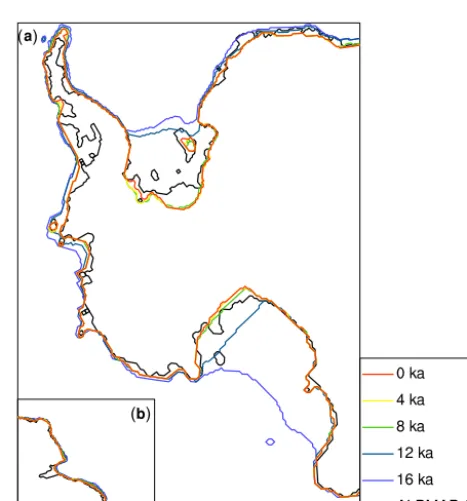
grounding lines at other time slices are shown here. The grounding line has moved very little along the EAIS, there-fore a zoom on the WAIS is shown in Fig. 7a. The grounding line on the western side of the Antarctic Peninsula has not re-treated far enough, which is probably also due to the low res-olution of the model. However, the PD grounding line along most of the rest of the coast, including the Ross Ice Shelf is well modelled in ANICE. The grounding line of the southern part of the Filchner–Ronne Ice Shelf has retreated too far in-land, but the timing of the onset of retreat (around 13 ka) is in agreement with Anderson et al. (2002). However, a more recent study by Weber et al. (2011) suggests that the onset of retreat took place around 19 ka in the Weddell Sea, which indicates a too-late retreat in ANICE. Additionally, they find that the margin of the ice shelf had retreated to half the length of the continental shelf around 14 ka and to its PD position around 11 ka, which does agree with the model results. The onset of the retreat of the Ross Ice Shelf is timed at 18 ka in ANICE. This is in accordance with the results of Ander-son et al. (2002), but they indicate that the PD position of the grounding line was not reached until 7 ka, while in ANICE the PD position is already reached around 10 ka. Addition-ally, the study by McKay et al. (2008) suggests a fast retreat of the Ross Ice Shelf between 11 and 10 ka. This fast retreat is also modelled by ANICE, but it is too early by about 3 kyr.
( )
( )
Figure 7. Grounding-line retreat from 16 ka until the PD, with in
black the PD grounding line from ALBMAP in (a) West Antarctica and (b) Prydz Bay (the Amery Ice Shelf region).
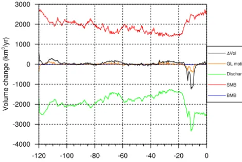
Figure 8. Evolution of the different contributions to grounded ice
volume change (in black): Grounding-line motion (orange), ice dis-charge over the grounding line (green), surface mass balance (red) and basal mass balance (blue).
In Sect. 4, results of the sensitivity experiments will be dis-cussed with the aid of the evolution of the grounded ice vol-ume for different simulations. Grounded ice volvol-ume change is attributed to SMB, BMB, ice discharge over the ground-ing line and groundground-ing-line retreat or advance. These four components are shown in Fig. 8 for the reference simulation. The BMB (in blue) gives a minor contribution to the ice vol-ume. The SMB (in red) and the discharge over the grounding line (in green) give the largest contributions, but as they are opposite and almost equal, their combined contribution is ap-proximately as large as the contribution of the grounding-line motion (in orange). Volume change (in black) is mostly posi-tive until the LGM, due to the SMB being slightly larger than the discharge and a gradual grounding-line advance. Around 16 ka the volume change becomes negative and stays nega-tive until the mid-Holocene. In the period from 16 to 7 ka the grounding line strongly retreats in the Weddell and Ross Seas (see Fig. 7) due to sea level rise. A lot of ice is then discharged over the grounding line, while the SMB is still growing to its PD level. At the PD, the ice discharge is al-most stable, albeit more pronounced than before the LGM. Grounding-line motion is negligible at the present, while the SMB seems to be still slightly growing.
4 Results of the sensitivity experiments
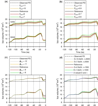
4.1 Ice-flow enhancement factors and basal stress The first sensitivity experiment involves the SIA enhance-ment factor. The evolution in time of the WAIS and EAIS ice volume for different values ofESIAis shown in Fig. 9a. The reference simulation is represented by the black solid line and the PD ice volume by the black dashed line. The ice volume in the figure is split into the volume of the EAIS
(upper part) and of the WAIS (lower part). The figure shows clearly that higher deformational velocities (largerESIA) lead to faster ice flow and therefore to less volume. The effect of changingESIA is strongest on the EAIS, where the move-ment of ice is mainly driven by deformation (Fig. 4). The PD ice volume is somewhat overestimated due to an overes-timation of the ice thickness on the Antarctic Peninsula, the Amery Ice Shelf region and the east coast of the Weddell Sea (Fig. 5c).
In the second sensitivity experiment, the SSA enhance-ment factor has been varied as shown in Fig. 9b. The fig-ure shows clearly that more sliding (largerESSA) leads to less volume. This is due to sliding causing the ice especially on the WAIS to flow faster and therefore the ice sheet loses more mass. The timing of the LGM is also different for dif-ferent values ofESSA. This is because high ice velocities are reached earlier in time for higher values ofESSA, preventing the ice sheet from advancing. Hence, the ice sheet starts re-treating earlier and therefore the LGM is timed earlier than for lower values ofESSA.
Between 9 and 5 ka, a minimum in ice volume is visible in all simulations in Fig. 9, especially for the EAIS volume. This dip is less pronounced in the simulations with less slid-ing, and it appears later. Other modelling studies that show the evolution of the grounded ice volume do not seem to find the same results (see for instance Philippon et al., 2006; Ritz et al., 2001), but there is sufficient observational evidence for a readvance as shown by Ingólfsson et al. (1998), Hall (2009), and Ackert Jr. et al. (2013), for example. From these studies it seems likely that the minimum should be timed around the mid-Holocene, which is consistent with the re-sults for φmin=10–12◦. Most of the grounding-line read-vance in ANICE is located on the eastern and western side of the Filchner–Ronne Ice Shelf and on the western side of the Ross Ice Shelf. This is in accordance with the observations, but other readvances that have been observed are not mod-elled (e.g. on the Antarctic Peninsula), due to the too coarse resolution of the model. This mid-Holocene readvance and, at other locations, stagnation of the grounding line leads to less discharge while the surface mass balance increases due to higher temperatures. Together, these two effects lead to an increase in ice volume.
( ) ( )
( ) ( )
Figure 9. EAIS (upper lines) and WAIS (lower lines) grounded ice volume from 120 ka until the present for different values of the (a) SIA
enhancement factor (ESIA), (b) SSA enhancement factor (ESSA), (c) sliding parameterφminand (d) flexural rigidity (D) and relaxation
time (τ), with an extra blue line indicating the simulation withD=5.0×1024Nm,τ=2000 yr for the WAIS andD=1.0×1025Nm,
τ=3000 yr for the EAIS. The reference simulation (black solid line) hasESIA=9,ESSA=0.8,φmin=10◦,D=5×1024Nm andτ=
2000 yr. Dashed lines have been drawn in black at the level of the PD grounded ice volume for both the EAIS and the WAIS.
4.2 Bedrock response
The effect of changing the flexural rigidity and the relaxation time on the ice volume evolution is shown in Fig. 9d. A thin-ner lithosphere implies both a smaller value for D and for
τ. As these two parameters are coupled, we chose to show the simulations where both parameters have been changed in the same direction. However, we have done simulations with independently varied D andτ, and it should be noted that the effect of varyingDis smaller than the effect of varying
τ, which indicates that the speed of the lithosphere reaction is more important for the evolution of the ice sheet than the amplitude.
From Fig. 9d it is clear that a thinner lithosphere leads to a higher PD ice volume, especially on the WAIS. Here, the largest changes in ice loading take place (relative with
sheet, but it is influenced by the higher values for Dandτ
used for the EAIS, leading to a slightly smaller PD ice vol-ume.
For the EAIS, there seems to be a threshold value between
D=1.0×1024Nm, τ=1000 yr and D=2.5×1024Nm,
τ =1500 yr, where the ice sheet hardly shrinks from the LGM to the PD. Because of this, the simulation withD= 1.0×1024Nm,τ =1000 yr is not regarded as realistic. The bedrock model parameters also have an influence on the ice volume minimum in the mid-Holocene. A thinner lithosphere causes a less pronounced dip which occurs later.
4.3 Ice volume and grounding-line retreat
In ALBMAP, the PD WAIS grounded ice volume is 8.1× 10⁶km3and the EAIS volume is 16.7×10⁶km3. Together they make up 24.8×10⁶km3of ice for the entire AIS. Both the WAIS and the EAIS PD grounded ice volume are overes-timated, by 1.3×10⁶km3and 0.7×10⁶km3respectively. A large part of the overestimation of the WAIS volume (about 30 %) is due to a too-low resolution to model the topography of the Antarctic Peninsula correctly, which can be seen from Fig. 5c.
The additional grounded ice volume present on the AIS during the LGM is estimated to be between 14 m and 24.5 m sea level equivalent (s.l.e.), or 5.6 to 9.8×10⁶km3by Clark and Mix (2002), about 8 m s.l.e. or 3.2×10⁶km3by White-house et al. (2012) and Golledge et al. (2013), between 6.3 and 10.5 m s.l.e. or between 2.5 and 4.2×10⁶km3by Briggs and Tarasov (2013) and between 7 and 9 m s.l.e. or between 2.8 and 3.6×10⁶km3by Gomez et al. (2013). This means there was 27.3 to 34.6×10⁶km3of ice present on the AIS at the LGM. For all simulations, the total AIS LGM ice volume falls within this range; the LGM grounded ice volume from our sensitivity simulations ranges between 30.5 and 32.4× 10⁶ km3. If the extremes are not taken into account (i.e. the results for φmin=8, φmin=12, ESIA=7, ESIA=11, ESSA=0.6,ESSA=1.0 and the upper and lower values for Dandτ), filtering out unrealistic simulations like the simu-lation withD=1.0×1024Nm,τ=1000 yr (see Sect. 4.2), the LGM grounded ice volume ranges between 31.0 and 31.8×10⁶km3. For these simulations, the change in ice vol-ume from the LGM to the PD is−4.3±0.5×10⁶km3which is equivalent to 10.7±1.3 m s.l.e. and falls within the range found in the literature. Our model predicts that the maximum ice volume on the AIS was reached between 15 and 16 ka, which is in good agreement with Verleyen et al. (2005), for example, who found that the maximum ice volume occurred at 16 ka.
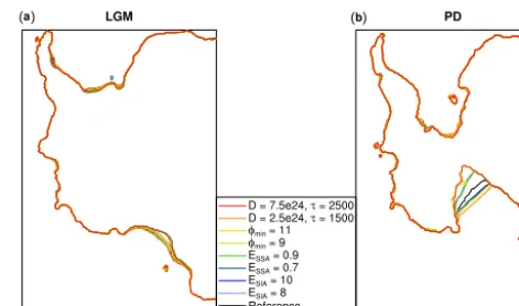
A comparison of the grounding-line positions at the LGM and the PD for different values of the investigated parameters is shown in Fig. 10. At the LGM, there is not much difference between the grounding-line positions because they are all close to the continental shelf and hence cannot advance fur-ther. Anderson et al. (2002) and Denton and Hughes (2002)
( ) ( )
Figure 10. Grounding-line positions at (a) the LGM, 16 ka and (b)
the PD, for the reference simulation and for simulations with varia-tions of the indicated parameters.
both show LGM grounding-line reconstructions, which agree with our modelled grounding-line positions. However, the grounding lines for theD=7.5×1024Nm, τ=2500 and theESSA=0.9 simulations seem to be located slightly too far inland from the Ross Sea. The PD grounding-line loca-tions only vary substantially in the Ross Sea, indicating that the Ross Ice Shelf is more sensitive than the Filchner–Ronne Ice Shelf. The location of the grounding line is strongly cor-related with the WAIS ice volume, that is, a lower WAIS ice volume with respect to the reference simulation is connected to a grounding line that is situated further inland.
5 Conclusions
We investigated the effect of the friction angle of the bed below sea level, the SSA and SIA enhancement factors and the flexural rigidity and the relaxation time of the bedrock on the evolution of the AIS. We did this by first defin-ing a reference simulation with the followdefin-ing settdefin-ings of the studied parameters:φmin=10◦,ESSA=0.8,ESSA=9, D=5.0×1024N m andτ =2000 yr. The reference simula-tion gives satisfactory results for the LGM and the PD. The effect of the aforementioned parameters has been tested by doing sensitivity experiments.
Furthermore, we studied the effect of changing the SIA en-hancement factor (ESIA) and two bedrock model parameters on the ice sheet. The effect of the SIA enhancement factor is mostly seen on the EAIS, where the ice moves due to defor-mation. A larger value ofESIAleads to less volume over the entire simulation period 120 ka–present.
The effect of the changes in the flexural rigidity and the relaxation time of the bedrock are most pronounced on the WAIS where the largest changes in ice loading take place. A thinner lithosphere (modelled by a smaller flexural rigidity and relaxation time) leads to a higher PD ice volume due to a faster rebounding of the bed, which causes a shallower grounding line and therefore a reduction in the ice flux across the grounding line.
We compared grounding-line positions for different sen-sitivity experiments. From this we conclude that the grounding-line position at the LGM is not very sensitive to changes in the investigated parameters. For the PD ice sheet, the largest differences occur for the grounding line in the Ross Sea. The grounding-line position is correlated to the WAIS ice volume, where a smaller PD ice volume is con-nected to a grounding line located further inland.
The maximum grounded ice volume for the entire AIS occurred between 15 and 16 ka and lies between 30.5 and 32.4×10⁶km3, which is within the range of 28.0 to 34.6× 10⁶km3 found in the literature. The PD grounded ice vol-ume is overestimated in the model by about 8 %, which is probably mainly due to the fact that with a resolution of 20×20 km the details of the topography of the Antarctic Peninsula and the Amery Ice Shelf area cannot be modelled correctly. The difference between the modelled LGM and the PD grounded ice volume is−4.3±0.5×10⁶km3, equivalent to 10.7±1.3 m s.l.e., which is also within the range found in the literature (8 to 24.5 m s.l.e.)
We conclude that ANICE performs well regarding the PD grounding line, grounding-line retreat and LGM grounded ice volume. The optimal set of parameters we used in this study to define the reference simulation can be applied to study the deglaciation of the AIS from LGM to PD in more detail. In such subsequent studies, it would be interesting to perform ensemble runs and compare results from ANICE to observations, as has been done by Briggs et al. (2013), for example.
Acknowledgements. The figures in this paper were produced with
NCL (UCAR/NCAR/CISL/VETS, 2013). We thank SURFsara (www.surfsara.nl) for the support in using the Cartesius Compute Cluster. Furthermore, computational resources required for exper-iments with HadCM3 have been provided by the supercomputing facilities of the Université catholique de Louvain (CISM/UCL). We also want to thank an anonymous reviewer, J. Fastook and the editor, E. Larour for their suggestions and detailed comments, which led us to significant improvements of the manuscript. Edited by: E. Larour
References
Ackert Jr., R., Putnam, A., Mukhopadhyay, S., Pollard, D., De-Conto, R., Kurz, M., and Borns Jr., H.: Controls on interior West Antarctic Ice Sheet Elevations: inferences from geologic con-straints and ice sheet modeling, Quaternary Sci. Rev., 65, 26–38, doi:10.1016/j.quascirev.2012.12.017, 2013.
Anderson, J., Shipp, S., Lowe, A., Smith Wellner, J., and Mosola, A.: The Antarctic Ice Sheet during the Last Glacial Maximum and its subsequent retreat history: a review, Quaternary Sci. Rev., 21, 49–70, 2002.
Aschwanden, A., Aðalgeirsdóttir, G., and Khroulev, C.: Hindcast-ing to measure ice sheet model sensitivity to initial states, The Cryosphere, 7, 1083–1093, doi:10.5194/tc-7-1083-2013, 2013. Bintanja, R. and van de Wal, R.: North American ice-sheet
dynam-ics and the onset of 100,000-year glacial cycles, Nature, 454, 869–872, doi:10.1038/nature07158, 2008.
Braconnot, P., Otto-Bliesner, B., Harrison, S., Joussaume, S., Pe-terchmitt, J.-Y., Abe-Ouchi, A., Crucifix, M., Driesschaert, E., Fichefet, Th., Hewitt, C. D., Kageyama, M., Kitoh, A., Laîné, A., Loutre, M.-F., Marti, O., Merkel, U., Ramstein, G., Valdes, P., Weber, S. L., Yu, Y., and Zhao, Y.: Results of PMIP2 coupled simulations of the Mid-Holocene and Last Glacial Maximum – Part 1: experiments and large-scale features, Clim. Past, 3, 261– 277, doi:10.5194/cp-3-261-2007, 2007.
Briggs, R. and Tarasov, L.: How to evaluate model-derived deglacia-tion chronologies: a case study using Antarctica, Quaternary Sci. Rev., 63, 109–127, doi:10.1016/j.quascirev.2012.11.021, 2013. Briggs, R., Pollard, D., and Tarasov, L.: A glacial systems model
configured for large ensemble analysis of Antarctic deglacia-tion, The Cryosphere, 7, 1949–1970, doi:10.5194/tc-7-1949-2013, 2013.
Bueler, E. and Brown, J.: Shallow shelf approximation as a “sliding law” in a thermomechanically coupled ice sheet model, J. Geo-phys. Res., 114, 1–21, doi:10.1029/2008JF001179, 2009. Clark, P. and Mix, A.: Ice sheets and sea level of the Last Glacial
Maximum, Quaternary Sci. Rev., 21, 1–7, 2002.
Clarke, G.: Subglacial Processes, Annu. Rev. Earth Pl. Sc., 33, 247– 276, doi:10.1146/annurev.earth.33.092203.122621, 2005. Crucifix, M., Loutre, M.-F., Lambeck, K., and Berger, A.: Effect of
isostatic rebound on modelled ice volume variations during the last 200 kyr, Earth Planet. Sc. Lett., 184, 623–633, 2001. De Boer, B.: A reconstruction of temperature, ice volume and
atmo-spheric CO2over the past 40 million years, Ph.D. thesis, Utrecht
University, Utrecht, 2012.
De Boer, B., van de Wal, R., Lourens, L., Bintanja, R., and Reerink, T.: A continuous simulation of global ice volume over the past 1 million years with 3-D ice-sheet models, Clim. Dynam., 41, 1365–1384, doi:10.1007/s00382-012-1562-2, 2012.
Denton, G. and Hughes, T.: Reconstructing the Antarctic Ice Sheet at the Last Glacial Maximum, Quaternary Sci. Rev., 21, 193–202, doi:10.1016/S0277-3791(01)00090-7, 2002.
Ettema, J., van den Broeke, M., van Meijgaard, E., van de Berg, W., Bamber, J., Box, J., and Bales, R.: Higher surface mass balance of the Greenland ice sheet revealed by high-resolution climate modeling, Geophys. Res. Lett., 36, L12501, doi:10.1029/2009GL038110, 2009.
Glen, J.: The flow law of ice: A discussion onf the assumptions made in glacier theory, their experimental foundations and con-sequences, IASH Publ., 47, 171–183, 1958.
Golledge, N., Fogwill, C., Mackintosh, A., and Buckley, K.: Dy-namics of the last glacial maximum Antarctic ice-sheet and its response to ocean forcing, P. Natl. Acad. Sci. USA, 109, 16052– 16056, doi:10.1073/pnas.1205385109, 2012.
Golledge, N., Levy, R., McKay, R., Fogwill, C., White, D., Graham, A., Smith, J., Hillenbrand, C.-D., Licht, K., Den-ton, G., Ackert Jr., R., Maas, S., and Hall, B.: Glaciol-ogy and geological signature of the Last Glacial Maxi-mum Antarctic Ice Sheet, Quaternary Sci. Rev., 78, 225–247, doi:10.1016/j.quascirev.2013.08.011, 2013.
Gomez, N., Pollard, D., and Mitrovica, J.: A 3-D cou-pled ice sheet – sea level model applied to Antarctica through the last 40 ky, Earth Planet. Sc. Lett., 384, 88–99, doi:10.1016/j.epsl.2013.09.042, 2013.
Hall, B.: Holocene glacial history of Antarctica and the sub-Antarctic islands, Quaternary Sci. Rev., 28, 2213–2230, doi:10.1016/j.quascirev.2009.06.011, 2009.
Holland, D. and Jenkins, A.: Modeling thermodynamic ice-ocean interactions at the base of an ice shelf, J. Phys. Oceanogr., 29, 1787–1800, 1999.
Huerta, A. and Harry, D.: The transition from diffuse to fo-cused extension: Modeled evolution of the West Antarc-tic Rift system, Earth Planet. Sc. Lett., 255, 133–147, doi:10.1016/j.epsl.2006.12.011, 2007.
Huybrechts, P.: The Antarctic ice sheet and environmental change: a three-dimensional modelling study, Berichte zur Polarforschung, 99, 1–241, 1992.
Huybrechts, P.: Sea-level changes at the LGM from ice-dynamic reconstructions of the Greenland and Antarctic ice sheets during the glacial cycles, Quaternary Sci. Rev., 21, 203–231, 2002. Ingólfsson, Ó., Hjort, C., Berkman, P., Björck, S., Colhoun, E.,
Goodwin, I., Hall, B., Hirakawa, K., Melles, M., Möller, P., and Prentice, M.: Antarctic glacial history since the Last Glacial Maximum: an overview of the record on land, Antarct. Sci., 10, 326–344, 1998.
Jouzel, J., Masson-Delmotte, V., Cattani, O., Dreyfus, G., Falourd, S., Hoffmann, G., Minster, B., Nouet, J., Barnola, J., Chappel-laz, J., Fischer, H., Gallet, J., Johnsen, S., Leuenberger, M., Loulergue, L., Luethi, D., Oerter, H., Parrenin, F., Raisbeck, G., Raynaud, D., Schilt, A., Schwander, J., Selmo, E., Souchez, R., Spahni, R., Stauffer, B., Steffensen, J., Stenni, B., Stocker, T., Tison, J., Werner, M., and Wolff, E.: EPICA Dome C ice core 800kyr deuterium data and temperature estimates, IGBP PAGES/World Data Center for Paleoclimatology data contribu-tion series 2007-091, NOAA/NCDC Paleoclimatology Program, Boulder CO, USA, 2007.
Knauss, J.: Introduction to physical oceanography, Prentice Hall, Upper Saddle River, New Jersey, 2 Edn., 1997.
Kuipers Munneke, P., van den Broeke, M., Lenaerts, J., Flanner, M., Gardner, A., and van de Berg, W.: A new albedo parameter-ization for use in climate models over the Antarctic ice sheet, J. Geophys. Res., 116, D05114, doi:10.1029/2010JD015113, 2011. Le Brocq, A. M., Payne, A. J., and Vieli, A.: An improved Antarctic dataset for high resolution numerical ice sheet models (ALBMAP v1), Earth Syst. Sci. Data, 2, 247–260, doi:10.5194/essd-2-247-2010, 2010.
Le Meur, E. and Huybrechts, P.: A comparison of different ways of dealing with isostasy: examples from modelling the Antarctic ice sheet during the last glacial cycle, Ann. Glaciol., 23, 309–317, 1996.
Lenaerts, J., van den Broeke, M., van de Berg, W., van Meijgaard, E., and Kuipers Munneke, P.: A new, high-resolution surface mass balance map of Antarctica (1979–2010) based on regional atmospheric climate modeling, Geophys. Res. Lett., 39, 1–5, doi:10.1029/2011GL050713, 2012.
Ligtenberg, S., van de Berg, W., van den Broeke, M., Rae, J., and van Meijgaard, E.: Future surface mass balance of the Antarctic ice sheet and its influence on sea level change, simulated by a re-gional atmospheric climate model, Clim. Dynam., 41, 867–884, doi:10.1007/s00382-013-1749-1, 2013.
Ma, Y., Gagliardini, O., Ritz, C., Gillet-Chaulet, F., Durand, G., and Montagnat, M.: Enhancement factors for grounded ice and ice shelves inferred from an anisotropic ice-flow model, J. Glaciol., 56, 805–812, doi:10.3189/002214310794457209, 2010. Maris, M. N. A., de Boer, B., and Oerlemans, J.: A climate model
intercomparison for the Antarctic region: present and past, Clim. Past, 8, 803–814, doi:10.5194/cp-8-803-2012, 2012.
McKay, R., Dunbar, G., Naish, T., Barrett, P., Carter, L., and Harper, M.: Retreat history of the Ross Ice Sheet (Shelf) since the Last Glacial Maximum from deep-basin sediment cores around Ross Island, Palaeogeogr. Palaeocl., 260, 245–261, doi:10.1016/j.palaeo.2007.08.015, 2008.
Morelli, A. and Danesi, S.: Seismological imaging of the Antarc-tic continental lithosphere: a review, Global Planet. Change, 42, 155–165, doi:10.1016/j.gloplacha.2003.12.005, 2004.
Orsi, A. and Whitworth III, T.: Hydrographic Atlas fo the World Ocean Circulation Experiment (WOCE) Volume 1: Southern Ocean, International WOCE Project Office, Southampton, U.K., 2004.
Pattyn, F., Schoof, C., Perichon, L., Hindmarsh, R. C. A., Bueler, E., de Fleurian, B., Durand, G., Gagliardini, O., Gladstone, R., Goldberg, D., Gudmundsson, G. H., Huybrechts, P., Lee, V., Nick, F. M., Payne, A. J., Pollard, D., Rybak, O., Saito, F., and Vieli, A.: Results of the Marine Ice Sheet Model Intercomparison Project, MISMIP, The Cryosphere, 6, 573–588, doi:10.5194/tc-6-573-2012, 2012.
Pattyn, F., Perichon, L., Durand, G., Favier, L., Gagliardini, O., Hindmarsh, R., Zwinger, T., Albrecht, T., Cornford, S., Doc-quier, D., Fürst, J., Goldberg, D., Gudmundsson, G., Humbert, A., Hütten, M., Huybrechts, P., Jouvet, G., Kleiner, T., Larour, E., Martin, D., Morlighem, M., Payne, A., Pollard, D., Rück-amp, M., Rybak, O., Seroussi, H., Thoma, M., and Wilkens, N.: Grounding-line migration in plan-view marine ice-sheet models: results of the ice2sea MISMIP3d intercomparison, J. Glaciol., 59, 410–422, doi:10.3189/2013JoG12J129, 2013.
Peltier, W.: Global glacial isostasy and the surface of the ice-age Earth: The ICE-5G (VM2) Model and GRACE, Annu. Rev. Earth Pl. Sc., 32, 111–149, doi:10.1146/annurev.earth.32.082503.144359, 2004.
Pollard, D. and DeConto, R.: Modeling West Antarctic ice sheet growth and collapse through the past five million years, Nature, 458, 329–332, doi:10.1038/nature07809, 2009.
Pollard, D. and DeConto, R. M.: Description of a hybrid ice sheet-shelf model, and application to Antarctica, Geosci. Model Dev., 5, 1273–1295, doi:10.5194/gmd-5-1273-2012, 2012a.
Pollard, D. and DeConto, R. M.: A simple inverse method for the distribution of basal sliding coefficients under ice sheets, applied to Antarctica, The Cryosphere, 6, 953–971, doi:10.5194/tc-6-953-2012, 2012b.
Ranalli, G.: Rheology of the Earth, Chapman & Hall, 2–6 Boundary Row, London, 2 Edn., 1995.
Ritz, C., Rommelaere, V., and Dumas, C.: Modeling the evolution of Antarctic ice sheet over the last 420,000 years: Implications for altitude changes in the Vostok region, J. Geophys. Res., 106, 31943–31964, 2001.
Stern, T. and ten Brink, U.: Flexural uplift of the Transantarctic Mountains, J. Geophys. Res., 94, 10315–10330, 1989.
UCAR/NCAR/CISL/VETS: The NCAR Command Language (Ver-sion 6.1.2) [Software], Boulder CO, doi:10.5065/D6WD3XH5, 2013.
Van de Berg, W., van den Broeke, M., Reijmer, C., and van Mei-jgaard, E.: Reassessment of the Antarctic surface mass balance using calibrated output of a regional atmospheric climate model, J. Geophys. Res., 111, D11104, doi:10.1029/2005JD006495, 2006.
Van Meijgaard, E., van Ulft, L., van de Berg, W., Bosveld, F., van den Hurk, B., Lenderink, G., and Siebesma, A.: The KNMI re-gional atmospheric climate model RACMO version 2.1, Royal Netherlands Meteorological Institute, De Bilt, the Netherlands, 2008.
Verleyen, E., Hodgson, D., Milne, G., Sabbe, K., and Vyver-man, W.: Relative sea-level history from the Lambert Glacier region, East Antarctica, and its relation to deglaciation and Holocene glacier readvance, Quaternary Res., 63, 45–52, doi:10.1016/j.yqres.2004.09.005, 2005.
Weber, M., Clark, P., Ricken, W., Mitrovica, J., Hostetler, S., and Kuhn, G.: Interhemispheric ice-sheet synchronicity dur-ing the Last Glacial Maximum, Science, 334, 1265–1269, doi:10.1126/science.1209299, 2011.
Whitehouse, P., Bentley, M., and Le Brocq, A.: A deglacial model for Antarctica: geological constraints and glaciolog-ical modelling as a basis for a new model of Antarctic glacial isostatic adjustment, Quaternary Sci. Rev., 32, 1–24, doi:10.1016/j.quascirev.2011.11.016, 2012.