www.clim-past.net/10/437/2014/ doi:10.5194/cp-10-437-2014
© Author(s) 2014. CC Attribution 3.0 License.
Climate
of the Past
Forward modelling of tree-ring width and comparison
with a global network of tree-ring chronologies
P. Breitenmoser1,2, S. Brönnimann1,2, and D. Frank2,3
1Institute of Geography, Climatology and Meteorology, University of Bern, Bern, Switzerland 2Oeschger Centre for Climate Change Research, University of Bern, Bern, Switzerland
3Swiss Federal Institute for Forest, Snow and Landscape Research (WSL), Birmensdorf, Switzerland Correspondence to: P. Breitenmoser ([email protected])
Received: 30 June 2013 – Published in Clim. Past Discuss.: 18 July 2013
Revised: 25 January 2014 – Accepted: 28 January 2014 – Published: 11 March 2014
Abstract. We investigate relationships between climate and
tree-ring data on a global scale using the process-based Vaganov–Shashkin Lite (VSL) forward model of tree-ring width formation. The VSL model requires as inputs only lat-itude, monthly mean temperature, and monthly accumulated precipitation. Hence, this simple, process-based model en-ables ring-width simulation at any location where monthly climate records exist. In this study, we analyse the growth response of simulated tree rings to monthly climate condi-tions obtained from the CRU TS3.1 data set back to 1901. Our key aims are (a) to assess the VSL model performance by examining the relations between simulated and observed growth at 2287 globally distributed sites, (b) indentify opti-mal growth parameters found during the model calibration, and (c) to evaluate the potential of the VSL model as an observation operator for data-assimilation-based reconstruc-tions of climate from tree-ring width. The assessment of the growth-onset threshold temperature of approximately 4–6◦C for most sites and species using a Bayesian estimation ap-proach complements other studies on the lower temperature limits where plant growth may be sustained. Our results sug-gest that the VSL model skilfully simulates site level tree-ring series in response to climate forcing for a wide range of environmental conditions and species. Spatial aggregation of the tree-ring chronologies to reduce non-climatic noise at the site level yielded notable improvements in the coherence between modelled and actual growth. The resulting distinct and coherent patterns of significant relationships between the aggregated and simulated series further demonstrate the VSL model’s ability to skilfully capture the climatic signal
contained in tree-ring series. Finally, we propose that the VSL model can be used as an observation operator in data assimilation approaches to reconstruct past climate.
1 Introduction
primarily limited by cold temperatures. This leaves the vast areas away from high mountains and high-latitude environ-ments poorly represented by high-quality temperature proxy data (Wahl and Frank, 2012).
In recent years, data assimilation approaches have found an increasingly important role in palaeoclimatic reconstruc-tion efforts (Hughes and Ammann, 2009; Trouet et al., 2009; Goosse et al., 2010; Widmann et al., 2010; Franke et al., 2011; Bhend et al., 2012; Tingley et al., 2012; Steiger et al., 2014; for an introduction and overview see Hakim et al. (2013) and Brönnimann et al. (2013)). Combining infor-mation from climate models and proxy archives, also includ-ing associated errors and their covariance, provides a physi-cally plausible representation of past climate consistent with available proxy data. An observation operator, which ex-presses the proxy as a function of the model data, is the for-mal link between model and proxy data. So-called forward proxy models (process-based or empirical) could potentially be used as an observation operator in data assimilation ap-proaches (Hughes and Ammann, 2009).
The Vaganov–Shashkin (VS; Vaganov et al., 2006, 2011) process-based forward model has been demonstrated to skil-fully simulate tree-ring width in North America and Siberia (Anchukaitis et al., 2006; Evans et al., 2006; Vaganov et al., 2011), China (Shi et al., 2008; Zhang et al., 2011), and Tunisia (Touchan et al., 2012). This forward-model of tree-ring growth was developed to quantify tree-ring forma-tion as a funcforma-tion of climate and environmental variables (Vaganov et al., 2006, 2011). Yet applications generating “pseudo ring-width” series from global climate models have so far been hindered by the complexity of forward models needed to accomplish this task. Recently, Tolwinski-Ward et al. (2011a, b) introduced a simplified model version (the so-called Vaganov–Shashkin Lite (VSL) model) that skil-fully reproduced climate-driven variability in North Amer-ican tree-ring width chronologies. This simple and efficient model of non-linear climatic controls on tree-ring width re-quires only latitude, monthly temperature, and monthly pre-cipitation as inputs and has the potential to simulate tree rings across a wide range of environments, species, and spa-tial scales. The VSL model may thus theoretically serve as a link between the proxy data and climate variables in any re-construction methodology that can support use of a forward model.
The goals of this study are to (a) to assess the VSL model performance by examining the relations between simulated and observed growth at 2287 globally distributed sites, (b) identify optimal growth parameters found during the model calibration, and (c) to evaluate the potential of the VSL model as an observation operator for data-assimilation-based reconstructions of climate from tree-ring width. This study is the first report examining the VSL model’s application on a global scale, and thereby across a wide range of species and site conditions, using a gridded data set based on direct observations from meteorological stations. All raw tree-ring
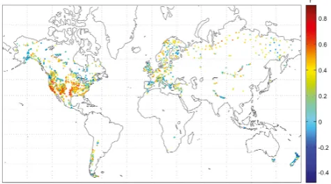
Fig. 1. Locations of the 2287 tree-ring width chronologies
(TRWITRDB)and the correlation coefficients between TRWITRDB and TRWVSLfor 1901–1970.
width measurements from the International Tree Ring Data Bank (ITRDB) are processed and analysed in a consistent manner.
The paper is organised as follows: we provide a brief in-troduction to the climate data, the structure and parameterisa-tions of the VSL model, and the tree-ring chronologies. The main results and discussion detailing the coherence between observed and simulated growth and associated climatic con-trols across space and over time are then presented. Finally, based on our findings, we discuss possible pathways of how tree-ring data could be used in data assimilation and climate reconstruction contexts.
2 Data and methods
2.1 Climate data
tree-ring network. Note that sites of tree-ring chronologies are, on average, located 164 m higher than the elevation of the corresponding CRU grid cell. Correction for elevational differences requires knowledge of the site-specific climato-logical lapse rate and is therefore difficult to achieve (e.g. tests assuming a constant moist-adiabatic lapse rate on a site-by-site basis did not improve fits between tree-ring and model data) and was not further considered.
2.2 Forward model description: the VSL model
We use the Vaganov–Shashkin Lite (VSL) model and a Bayesian parameter estimation approach (Tolwinski-Ward et al., 2013) to produce synthetic tree-ring chronolo-gies (Tolwinski-Ward et al., 2011a, b; version 2.3 acces-sible from http://www.ncdc.noaa.gov/paleo/softlib/softlib. html). The VSL model only requires monthly mean tem-perature, accumulated precipitation, and latitude to model growth. A further 12 adjustable parameters are required re-lated to climatic limitations on growth, parameterisations for soil moisture availability, and the calendar periods when an-nual increment of wood is responsive to climate. The net ef-fect of the dominating non-linear climatic controls on tree growth are implemented in terms of the principle of limiting factors and threshold growth response functions.
For a specific site and given monthi, growth is calculated from the minimum of the growth responses to temperature (gT)and moisture (gM), modulated by the response to inso-lation (gE):
G (i)=gE(i)∗min{gT(i) , gM(i)}. (1)
Annual ring width is then defined as the sum of the monthly growth increments G(i) over a specified growth period I
(Tolwinski-Ward et al., 2011a): TRWVSL=
X
i∈I
G(i). (2)
In Eq. (1),gEis the ratio of mean monthly day lengthL rela-tive to that in the summer solstice month at the corresponding latitude, computed using standard trigonometric approxima-tions:
gE(i)=
L(i)
max{L(i)}. (3)
The partial growth ratesgT andgM are defined as ramp func-tions, with growth parameters representing climate thresh-olds below which temperature T and moisture M are not high enough for growth (T1, M1), and thresholds above which temperature or moisture sustain non-limited growth (T2, M2). Values of these partial growth responses are be-tween zero and one (Tolwinski-Ward et al., 2011a):
gT(i)=
0 forT (i)≤T1 T (i)−T1
T2−T1 forT1< T (i)≤T2
1 forT (i) > T2
(4)
gM(i)=
0 forM (i)≤M1 M(i)−M1
M2−M1 forM1< M(i)≤M2
1 forM (i) > M2
. (5)
Site-specific growth parameters (T1, T2, M1, and M2) are necessary due to diverse environmental conditions, site ecologies, and species represented in this global network. Accordingly, the VSL growth response function parame-ters were determined for each chronology via Bayesian pa-rameter estimation using temperature, precipitation, site lati-tude, and ring-width data during the calibration interval. This scheme assumes uniform priors for the growth response pa-rameters, and independent, normally distributed errors for the ring-width model. The median of each of the growth parameters in the resulting posterior probability distribution was finally taken as the “calibrated” growth response values for a particular site. A more detailed description of the ap-proach can be found in Tolwinski-Ward et al. (2013). The Bayesian approach is computationally efficient, is able to incorporate expert knowledge about the likely values for parameters, and tends to guard against model overfitting (Tolwinski-Ward et al., 2013).
In addition to the above-described Bayesian approach to estimate the optimal growth parameters, we also estimated the optimal growth parameters for every site using a sim-ple optimisation procedure as described in Tolwinski-Ward et al. (2011a). Growth parameters in this optimisation approach were sampled uniformly across intervals, and the growth pa-rameter set producing the simulation that correlated most sig-nificantly with the corresponding observed series was then used to simulate the tree-ring series (note that throughout this paper we use Pearson’s correlation coefficients). Results from both growth parameter estimation approaches are gen-erally similar. There was some evidence that the optimisa-tion approach sometimes overfit the model due to the lack of independence between the fitting procedure and the tree-ring–VSL relationships. Nevertheless, the comparable results support the validity of either of these approaches with some possible advantages for the Bayesian parameter estimation (Tolwinski-Ward et al., 2011a, 2013).
Soil moistureM(i)is calculated from monthly tempera-ture and accumulated precipitation data,T (i)andP (i),via the empirical Leaky Bucket model of hydrology from the National Oceanic and Atmospheric Administration’s Climate Prediction Center (CPC), allowing for sub-monthly updates of soil moisture to account for the non-linearity of the soil moisture response (Huang et al., 1996; Tolwinski-Ward et al., 2011a; codes available from http://www.ncdc.noaa.gov/ paleo/softlib/softlib.html).
Table 1. VSL model parameters.
Parameter description Parameter Value
Temperature response parameters
Threshold temp. forgT>0 T1 ε[1◦C, 9◦C] Threshold temp. forgT= 1 T2 ε[10◦C, 24◦C] Moisture response parameters
Threshold soil moist. forgM>0 M1 ε[0.01, 0.035] v/v Threshold soil moist. forgM=1 M2 ε[0.1, 0.7] v/v
Soil moisture parameters
Runoff parameter 1 α 0.093 month−1
Runoff parameter 2 µ 5.8 (dimensionless) Runoff parameter 3 m 4.886 (dimensionless) Max moisture held by soil Wmax 0.8 v/v Min moisture held by soil Wmin 0.01 v/v
Root (bucket) depth dr 1000 mm
Integration window parameters
Integration start month I0 −4
Integration end month If 12
Tolwinski-Ward et al., 2011a; Zhang et al., 2011; Touchan et al., 2012), as is outlined in Table 1, which have demonstrated the applicability of VSL for a wide range of environmental conditions.
As growth period, I, we use a 16-month interval, start-ing in the previous September and endstart-ing in December of the modelled year (previous March to current June for the Southern Hemisphere). This integration interval accounts for some persistence in tree-ring growth (leading to autocor-relation) and showed the best overall performance in tests from a subset of our data set (which are all sites in Africa, New Zealand, Tasmania, Chile, Mongolia, southeastern Asia, Austria, Norway, Florida, and California). This interval is furthermore consistent with the outcomes from Tolwinski-Ward et al. (2011a) in their simulations of North American tree-ring series and with the importance of autumn phenol-ogy controlling interannual variability of net ecosystem pro-ductivity (Wu et al., 2013).
2.3 Tree-ring chronologies
A total of 2287 standardised tree-ring chronologies were used for our primary analyses. To obtain these series, we considered all available raw tree-ring width measurements from 2918 sites from 163 different tree species from the ITRDB (Grissino-Mayer and Fritts, 1997; http://www.ncdc. noaa.gov/paleo/treering.html). Prior to further analysis, we attempted to identify and correct data and metadata errors including repetitive measurements, feet-meter encoding, in-appropriate decimal points and hyphenations, incorrect series labelling, or misplaced series positions (see Table S1 in the Supplement).
To remove the biological age trend and other lower-frequency signals that may be driven by stand dynamics
or disturbances, we processed all data sets in the program ARSTAN (Cook, 1985) using standard dendroclimatologi-cal methods (i.e. detrending and standardisation to dimen-sionless growth indices). We tested different standardisation methods on a subset of 97 locations from all six continents and selected our detrending approach based on this subset. Methods tested include (a) a negative exponential curve and linear regression fits, (b) a smoothing spline fit with a 50 % frequency response cut-off (which is the wavelength at which 50 % of the amplitude of a signal is retained) equal to three-fourths of a series length, and (c) a smoothing spline with a 200 yr frequency response cut-off. These tests and Pearson’s correlation analyses between the differently standardised se-ries and the monthly climate parameters led us to favour a hi-erarchical approach: fitting negative exponential curves and linear regression curves of any slope were applied as first-order detrending options; but if these two methods were not suitable (e.g. because values of a fitted curve approached zero), a smoothing spline was fit with a 50 % cut-off fre-quency at 75 % of each series length. The detrending meth-ods applied allow retention of climate-related signals in any given chronology of the order of the median segment length of the constituent tree-ring series (Cook et al., 1995).
Combining multiple measurements into a single ring-width chronology should then ideally represent a coherent climate signal of a particular species at a site (Cook et al., 1990). Standard chronologies (TRWITRDB)of all these sites were developed by a biweight robust mean estimate (Cook et al., 1990) and the variance was stabilised to minimise arte-facts from changing sample size through time (Osborn et al., 1997; Frank et al., 2007). Further, we required that the sample depth of a chronology (number of samples from trees used for every point in time) is always≥8 and that the 1901– 1970 interval was fully covered by tree-ring data. These cri-teria resulted in the 2287 chronologies for further analyses.
2.4 Aggregation of observed tree-ring chronologies
In addition to comparing individual observed and VSL-modelled chronologies, we further analysed whether the signal-to-noise ratio can be enhanced by aggregating several neighbouring observed series into one “super-chronology”, which subsequently is modelled with VSL.
one chronology must be within 200 km of a grid cell such that both search radii result in the same spatial coverage.
In contrast to modelling individual chronologies, mod-elling aggregated chronologies requires a first-order sepa-ration of the climatic influences on growth into “moisture-limited” and “temperature-“moisture-limited” chronologies to enhance the signal-to-noise ratio. Note that this aggregation approach means that changes in the limitations over time cannot be accounted for as might apply to the debate over the so-called “divergence phenomena” (D’Arrigo et al., 2008; Es-per and Frank, 2009). Yet, site aggregation is particularly important in mountainous terrain with more complex cli-matic conditions and rapidly changing conditions within small spatial scales that locally impact tree growth (Salzer and Kipfmueller, 2005). Accordingly, we differentiated the sites based upon their principal climatic drivers and thus separately aggregated all temperature- and moisture-limited chronologies located within each grid cell node’s search ra-dius. Specifically, we classified temperature- and moisture-sensitive chronologies using the long-term averaged monthly growth responses gT and gM from the VSL model for all months where g >0. Temperature-sensitive chronolo-gies were defined as sites that have more temperature- than moisture-limited months (i.e. a greater number of months wheregT > gM). All other series are moisture-limited (equal or more months withgT> gM). Aggregated tree-ring width (ATRW) series for temperature- and moisture-limited se-ries were computed for every grid cell with one or more temperature and/or moisture-limited tree-ring chronologies located within the given search radius. For the 200 km (600 km) search radii, 10 % (7 %) of all land grid cells contain only temperature-limited series, 7 % (5 %) are only moisture-limited, and 11 % (37 %) of the cells include both temperature- and moisture-limited chronologies.
After identifying the series to be aggregated, we defined the aggregated tree-ring width ATRWITRDB as weighted means of the corresponding TRWITRDBseries. Weights were assigned according to four factors (Eqs. 6–9), and multipli-cation of the four relative weights gives the weight value we apply to each individual tree-ring series within the search radius. The weighting factors are (a) mean Rbar of each chronology, (b) mean EPS of each chronology, (c) distances
d between the site location and the grid node, and (d) the smaller p value of two correlations between CRUTS3.1 temperature or precipitation and TRWITRDB: for 12-month averages (January–December in the Northern Hemisphere, July–June in the Southern Hemisphere, respectively) and for 5-month averages for growing season interval (May– September and November–March, respectively). These two seasonal windows consider the summer months when cli-mate generally dominates tree growth (Briffa et al., 2002a) and also possibilities that growth is driven by a much wider seasonal window.
Weights are determined by to following functions (see Fig. S1), which vary between 0 and 1:
wRbar=e−2(1−Rbar)
5
(6)
wEPS=e−2(1−EPS) (7)
wd=e
−2d2
R2 (8)
wp=e−2p. (9)
There is no a priori reason to choose any particular weigh-ing function, but we determined the functions based on the-oretical considerations (e.g. see Ljungqvist et al., 2012, who used the Gaussian distance) and the parameter distribution as shown in Table 1. We re-calibrated the VSL simulations for all grid cells containing at least one aggregated tree-ring se-ries. The calibration was performed using monthly temper-ature and precipitation series from CRU and with the same VSL model parameter set-up described in Table 1.
2.5 Experimental and analysis design
The following experimental design is used in our study. First, we modelled (following Sect. 2.2) each individual ob-served chronology with data from the closest CRU grid cell as climatic input. These simulated chronologies are termed TRWVSL. In addition, we also modelled the aggregated chronologies using climate data from the centre of the search radius (closest grid cell), but calibrated using the aggregated observed chronologies ATRWITRDB. These chronologies are termed ATRWVSL. All observed and modelled chronologies were normalised (i.e. given a mean of zero and standard de-viation of unity) over the 1901–1970 period.
For both TRWVSLand ATRWVSL, we utilised 1901–1970 as the main calibration period for the growth parameters. However, for assessing result consistency, we also performed split-sample validation experiments in which we used the 1901–1935 period for calibration and the 1936–1970 period for validation and vice versa.
3 Results
3.1 Quality indicators for tree-ring chronologies
Fig. 2. Binned chronology characteristics for 1901–1970. Rbar is
the average inter-series correlation between all series from different trees (Cook et al., 1990); EPS is the expressed population signal and the vertical dashed line denotes the commonly cited 0.85 EPS criterion (Wigley et al., 1984; Cook et al., 1990). Mean 1901–1970 Rbar and EPS values were calculated using a 30 yr window that lags 15 yr; MSL is the mean segment length; and ASD is the average sample depth (48 bins were distinguished in each variable).
et al., 1984; a threshold value of 0.85 is routinely, but ar-bitrarily, cited in dendrochronological literature). Rbar and EPS statistics were calculated over moving 30 yr windows with 15 yr overlap. A total of 93 % of all mean EPS values in our network are above 0.85 over the 1901–1970 time pe-riod. Rbar values roughly follow a normal distribution with a mean of 0.39. These statistics suggest that the vast major-ity of chronologies have a relatively robust signal that should allow climatic drivers to be inferred. On average tree-ring chronologies are composed of 30 series with a mean segment length of 170 yr. However, these distributions have relatively long tails reflecting sites that are exceptionally well repli-cated or composed of long-lived tree species (e.g. Bristlecone pine). The mean segment length and our detrending approach suggest that we should be able to test inter-annual to (at least) multi-decadal variability in our modelling efforts. The geo-graphical distribution of the sites is dominated by low alti-tudes and the mid-latialti-tudes, but there are also a considerable number of high-latitude and high-elevation sites particularly in the Northern Hemisphere.
3.2 Site-specific Bayesian parameter estimation
The Bayesian approach provides estimates of the optimal parametersT1, T2, M1, andM2 for each site, with descrip-tive statistics of the parameter estimation for split-sample validation given in Table 2. Notably, we find great consis-tency among the temperature and moisture parameters that were calculated independently and separately for the 1901– 1935 and 1936–1970 periods. We find for example that the mean temperature for growth onset is 4.6 and 4.8◦C for the early and late calibration periods. Similarly, temperature no longer limited growth above 16.3 and 16.5◦C again for the independent early and late calibration periods. Figure 3
fur-Fig. 3. Histogram of the Bayesian estimated VSL growth response
parameters: (a) T1, lowest threshold temperature; (b) T2, lower bound for optimal temperature; (c)M1, lowest threshold for mois-ture; (d)M2, lower bound for optimal moisture parameters cal-culated during 1911–1970 for different tree genera: pine (pinus; n=821), spruce (picea; n=407), fir (abies; n=286), hemlock (tsuga;n=124), larch (larix;n=126), cedar (cedrus; n=107), juniper (juniperus; n=40), oak (quercus; n=253), and south-ern beech (nothofagus; n=62). Histogram of T1 threshold tem-perature for different pine species (e): Scots pine (Pinus sylvat-ica;n=172), Austrian pine (Pinus negra;n=45), ponderosa pine (Pinus ponderosa; n=181), pinyon pine (Pinus edulis;n=73), bristlecone pine (Pinus aristata, Pinus longaeva, and Pinus bal-fouriana;n=34), stone pine (Pinus pinea;n=7), and jack pine (Pinus banksiana;n=15). Numbers in brackets give the series con-tributing in each group of tree genera. The number of bins for each parameter is determined through the square root of its length.
ther illustrates the estimated temperature and moisture pa-rametersT1, T2, M1,andM2for each site and different tree genera. In terms of the currently debated (see Discussion) growth-onset threshold temperature (T1), we find most esti-mates fall within 4–6◦C with values for all sites and species between 1.80 and 8.41◦C (see also Table 2). Despite the generally narrow range of the parameters for all study sites, some evidence for species-dependent values also exists. For spruce, our estimates ofT1andT2are generally higher than for pine trees, while M2 is lower. We also find differences among the pine species. For ponderosa and pinyon pines,T1 is about 1 to 2◦C lower than for other pine species (Fig. 3e, compare also to Fig. 3a in which these two species clearly influence the shape of the pine histogram towards cooler threshold temperatures).
Table 2. Statistics of the Bayesian estimation of the site-by-site tuned VSL growth response parametersT1,T2,M1, andM2for the 1901– 1935 and 1936–1970 calibration intervals.
Calib. 1: 1901–1935 Calib. 2: 1936–1970
Mean Min Max SD Mean Min Max SD
T1(◦C) 4.64 1.80 8.41 0.93 4.75 1.74 7.97 0.89 T2(◦C) 16.34 10.14 22.80 1.62 16.52 10.36 21.87 1.59 M1(v/v) 0.023 0.02 0.025 0.001 0.023 0.019 0.025 0.001 M2(v/v) 0.44 0.11 0.64 0.09 0.43 0.11 0.64 0.09
values are significantly correlated with each other (r=0.60 and r=0.47, bothp <0.01). The often negative correla-tion between temperature and precipitacorrela-tion at inter-annual time scales is expressed by the inversely related tempera-ture and moistempera-ture growth parameters, with the relationship betweenT2 andM2 (r= −0.63,p <0.01) being the most noteworthy. Moreover, temperature-limited sites tend to have higher T1 and T2 values in comparison to the moisture-limited sites, whereas higherM1andM2values are charac-teristic of moisture-limited sites (please refer to Sect. 2.4 for the definition of temperature- and moisture-limited sites).
3.3 Relationships between actual and simulated
tree-ring growth
The VSL model was able to simulate tree-ring series for 2271 out of the 2287 sites, suggesting general applicability to di-verse environments and species. Of the remaining 16 sites, nine were high-latitude or high-elevation sites in Nepal (3), Siberia (1), and Canada/Alaska (5) for which no growth was simulated because temperatures never reached the threshold temperatureT1for growth initiation (hencegT =0). The re-maining seven sites were (sub-)tropical sites in Florida (1), Mexico (4), Argentina (1), and Indonesia (1), for which nei-ther temperature- nor moisture-limited growth (hencegT =1 andgM=1).
Similarity between the 2271 actual TRWITRDB and the corresponding modelled TRWVSLchronologies was assessed by Pearson’s correlation coefficients during the 1901–1970 period (Fig. 1). The average of Pearson’s correlation coeffi-cients between all TRWITRDBand TRWVSLis 0.29 (standard deviation=0.22). Approximately 41 % of the correlation co-efficients between TRWVSL and TRWITRDBare statistically significant at the 95 % confidence level (r >0.35), taking into account the reduction of degrees of freedom due to au-tocorrelation (Mitchell Jr. et al., 1966). Note, however, that the 1901–1970 period includes the calibration interval. Thus, analysing the correlation coefficients between TRWITRDB and TRWVSL in the split-sample validation, we find signif-icant (p=0.05;r >∼0.44) correlations during all four cali-bration/validation intervals (calibration 1901–1935 and vali-dation 1936–1970 and vice versa) for 13.3 % of all the series.
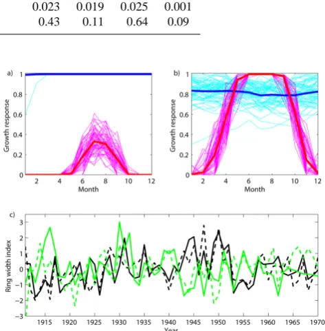
Fig. 4. Simulated monthly growth response curves for each year
(1911–1970) for temperature (gT, magenta lines) and moisture
(gM, cyan lines) for two sites in Switzerland: (a) Bergün Val Tuors,
European larch, 2065 m, and (b) Krauchthal, Scots pine, 550 m. The long-term (1911–1970) mean value is overlaid in red for tempera-ture and in blue for moistempera-ture; (c) TRWITRDBand TRWVSL(dashed lines) for Bergün Val Tuors (black lines),r=0.69,p <0.01 and Krauchthal (green lines),r=0.44,p <0.01.
Significant pairwise relationships between the TRWITRDB and TRWVSL series are found across the globe on all con-tinents. In particular, geographic areas with tendencies for higher model–data agreement are found in central Europe, Scandinavia, eastern/central Siberia and in the United States with a cluster of high correlations in California wherer >
0.8. Weak relationships are characteristic of the Africa sites, but are also evident in New Zealand, Tasmania, Alaska, a NW/SE band from central Canada to NE USA, the northern part of the British Isles, and parts of southern Europe (Fig. 1). To illustrate the monthly growth response values,gT and
month-wise minimum of either temperature or precipitation, Fig. 4a clearly shows that growth at the high-altitude site is temperature-limited (gT< gM). The lower-elevation site (Fig. 4b), on the other hand, is temperature-limited only briefly at the beginning and at the end of the growing sea-son, while precipitation limits growth during the summer months (gM< gT). Importantly, tree growth at the high-elevation site is negatively correlated with growth at the lower-elevation site. This negative correlation holds for both the observed and modelled chronologies with coefficients of −0.13 and −0.44, respectively. These relationships demon-strate the VSL model’s ability to incorporate joint influences of temperature and precipitation on growth, and simulta-neously suggest care is required when developing regional tree-ring time series (see Sect. 3.4.2 below). Our simulated growth responses for two selected sites in Switzerland ap-pears to be widely applicable across mountainous forest re-gions with large climatic gradients such as the southwest-ern USA (Salzer and Kipfmueller, 2005; Tolwinski-Ward et al., 2011a) and Mongolia (Poulter et al., 2013). One-year lagged autocorrelation coefficients (AR1) were assessed from TRWITRDBand TRWVSLseries at all sites. Mean coeffi-cients of 0.46 and 0.42, respectively, over all series clearly reveal persistence; i.e. 21 and 18 %, respectively, of the vari-ance in the width of the ring in the current year can be pre-dicted based upon simulated growth during the past year.
3.3.1 VSL simulations for aggregated TRW series
The aggregation generally enhances the correlation between ATRWVSL and ATRWITRDB. For instance, the average of all coefficients for R=200 km during the common 1901– 1970 interval is 0.34 for the temperature-limited series and 0.38 for the moisture-limited series compared with a mean of 0.29 for the non-aggregated tree-ring series. The spa-tial patterns of correlation coefficients for temperature- and moisture-limited ATRW for both search radii are shown in Fig. 5. Notably, ATRWVSL and ATRWITRDB show spatial coherency and capture the main climate signals and are thus suitable for data assimilation approaches (see Discus-sion). The 600 km search radius improves the relationships for both temperature and precipitation. Coherent regional-scale correlation patterns for temperature-limited series can be found in Scandinavia, western/central Siberia, and along the western and eastern United States (Fig. 5a and c). Re-gional correlation patterns for moisture-sensitive series en-compass the United States and central Canada (Fig. 5b and d). Regions such as central Europe, Turkey, central Asia, and the Andes are characterised by both temperature and mois-ture limitations, which is an expression of a complex terrain with small-scale climatic features and large climatic gradi-ents. High correlation coefficients between ATRWVSL and ATRWITRDB are present in all those regions, with a clear tendency towards temperature-limited, high-elevation sites. Poor agreement for the temperature-limited series can be
Fig. 5. World map displaying Pearson’s correlation coefficients
be-tween ATRWVSLand ATRWITRDBfor a search radius of 200 km
(a, b) and 600 km (c, d) at temperature-limited (a, c) and
P. Breitenmoser et al.: Forward modelling of tree-ring width 445
31
ITRDB
2
and moisture-limited (b,d) grid cells. Note that in panels c) and d) at least one chronology has 3
to be within the 200km search radius to make the correlations comparable. 4 5 6 7 8 9 10 11
Fig. 6. Scatter plot of correlation coefficients between each ATRWVSL and ATRWITRDB (200 km
12
search radius)series for the 1901-1935 and 1936-1970 independent time periods. Results are 13
shown for a) the early 1901-1935 calibration interval and b) the late 1936-1970 calibration 14
interval. 15
-1 -0.5 0 0.5 1 -1 -0.8 -0.6 -0.4 -0.2 0 0.2 0.4 0.6 0.8 1 a) b) -1 -0.8 -0.6 0 0.2 0.4 0.6 0.8 1 -0.4 -0.2
-1 -0.5 0 0.5 1 r during calibration 1901-35 r during calibration 1936-70
r d u ri n g v a li d a ti o n 1 9 3 6 -7 0 r d u ri n g v a lid a ti o n 1 9 0 1 -3 5
Fig. 6. Scatterplot of correlation coefficients between each
ATRWVSLand ATRWITRDB(200 km search radius) series for the 1901–1935 and 1936–1970 independent time periods. Results are shown for (a) the early 1901–1935 calibration interval and (b) the late 1936–1970 calibration interval.
found in Tasmania, New Zealand, western-central Canada, and in the eastern-central US, while moisture characteristics are poorly captured in Patagonia, northern Canada and in the European Alps.
Based on the split-sample validation experiment, Fig. 6 shows a scatterplot of the correlation coefficients between the ATRWVSL and ATRWITRDB, 200 km search radius, during different calibration/validation intervals (1901–1935/1936– 1970, and 1936–1970/1901–1935). Points along the 1:1 line are sites for which VSL produces simulations that are sta-ble in time, whereas points below this line represent sites for which the model yields a higher correlation during the calibration period. We find model skill (r >0.44) in Pear-son’s correlation coefficients in 36 % of the series during the calibration period, of which 54 % are also significant in the validation period. Correlations are stable for moisture-limited sites in large areas of the United States and cen-tral Canada, the lower-elevation sites in west-cencen-tral Eu-rope, Turkey, Mongolia, the western Himalayas, and in mid-Chile, whereas temperature-limited sites dominate Scandi-navia, Siberia, the eastern Himalayas, central Europe, south-ern South America, and parts of the westsouth-ern United States. Correlations are not particularly skilful for New Zealand, Tasmania, and Patagonia.
4 Discussion
4.1 Growth parameters
The site-by-site parameterisation for the moisture and tem-perature thresholds revealed interesting global-scale patterns. Notably, the parameter estimation of the VSL model pro-vides novel insights into the currently debated temperature threshold below which growth may no longer take place. Our estimations of growth-onset temperature (ca. 4–6◦C) is in agreement with the temperature range found by Tolwinski-Ward et al. (2013), who used a four-parameter beta distribu-tion to calibrate the model parameters on a subset of 277
se-ries in the United States. More striking is the convergence of findings with assessments of growing season temperatures at tree line based upon in situ loggers or remote sensing and in-terpolated climatic data (Körner and Paulsen, 2004; Körner, 2012), as well as observational studies of wood formation (Rossi et al., 2007). The wide range (1–9◦C) of the priors considered in our approach allowed ample room for devia-tion from the previous literature, so we interpret the agree-ment from these various lines of evidence as strong support for growth onset thresholds near 5◦C.
At the level of individual species or individual sites, our results compare well with findings of Vaganov et al. (2006), who, based on the VS model, reported minimum and opti-mal temperatures in the northern Taiga of 4 and 16◦C for larch, 6 and 18◦C for spruce, and 5 and 18◦C for Scots pine, respectively. The differences in growth thresholds might re-flect the better adaption of pines to lower-temperature con-ditions and drought. A comparison of the site values of the threshold temperatureT1at the corresponding elevations for different tree genera is shown in Fig. S2 in the Supplement. Species-related difference in moisture parameters may be due to needle structure as well as frequency and density of stomata which influence water loss due to evapotranspira-tion (Vaganov et al., 2006). Our results contribute to under-standing species specific growth responses as recently docu-mented in an analysis of 36 species from across the European continent (Babst et al., 2013).
At the same time, uncertainties arise from the parameter-isation of M and estimation of M1 and from the missing representation of winter precipitation stored as snowpack in the CPC Leaky Bucket model and its impact on the timing of snowmelt (Tolwinski-Ward et al., 2011a). Temperature-limited sites tend to have higherT1 andT2 than moisture-limited sites and vice versa for M1 andM2. This may be an expression of different climatic conditions, but may also be related to edaphic conditions and plant physiological dif-ferences. Figure S3 of the Supplement shows scatterplots of joint posterior relationships at each site between parameters (a)T1andT2, (b)M1andM2, (c)T2andM2, and (d)T1and
M1. Application of the VSL model in more controlled frame-works, such as in stands with mixed species compositions, will be useful to isolate and define species-specific growth characteristics while simultaneously excluding the possibili-ties that non-uniform species distributions along elevational gradients contribute to systemic differences in the obtained model parameters.
4.2 Relationships between actual and simulated growth
The broad-scale pattern of temperature-limited growth for high latitudes (e.g. Taymyr Peninsula, Russia), and high al-titudes (e.g. the European Alps) extends previous analyses of subsets of the ITRDB network (e.g. Briffa et al., 2002a; Wettstein et al., 2011; Babst et al., 2013). Our findings fur-thermore largely match the distribution of potential climatic constraints to plant growth in Nemani et al. (2003) and Beer et al. (2010) as well as the climate classification based on Köppen-Geiger by Kottek et al. (2006).
However, also prominent in our analysis were locations (e.g. Tasmania and New Zealand) where VSL simulations revealed little skill. To explore possible reasons for this we conducted initial simulations where climate variability was forced from a reanalysis product (20CR; Compo et al., 2011) and from the individual climate stations themselves. We found some evidence for improved skill which suggests that (a) the quality of the instrumental data sets and (b) strong orographic effects can affect our simulations. Caution is par-ticularly warranted where the quality and quantity of instru-mental stations rapidly decreases back in time (e.g. much of the Mediterranean, Asia, and Southern Hemisphere loca-tions with low population density and/or strong orographic effects).
The fact that VSL reproduces first-order autocorrelation structures (AR1) similar to the actual tree-ring chronologies highlights the importance of including last year’s growing season for growth simulation in the VSL model in order to retain potentially useful climate information contained in tree rings (see Table 1). Similarly, Wettstein et al. (2011) re-port median first-order autocorrelation coefficients of 0.47 for 762 ITRDB-derived tree-ring width series located pole-ward of roughly 30 to 40◦northern latitude, while Tingley et
al. (2012) found first-order autocorrelation coefficients of ap-proximately 0.6 for the tree-ring width series used in Mann et al. (2008). This reasonable agreement between the auto-correlation structure in actual versus simulated tree-ring data suggests that mechanistic modelling may help to reduce the effect of biases in the spectral characteristics of tree-ring chronologies on climate reconstructions (Meko, 1981; Cook et al., 1999; Franke et al., 2013). The global applicability of a 16-month seasonal window as applied herein will require further assessments for individual regions and species (for instance as in Wu et al., 2013). It is also conceivable to ap-ply differential weighting to previous years’ growth, but such schemes would be best implemented when understanding of lagged physiological processes and the roles of carbon re-serves are further advanced (e.g. Babst et al., 2013; Zielis et al., 2013).
4.3 Use of VSL in data assimilation
The favourable calibration–validation statistics of the VSL model and its ability to skilfully simulate growth for a wide range of environments suggest that the model could possi-bly be used for data assimilation approaches. In the
follow-ing section, several pathways are briefly outlined (see also Brönnimann et al., 2013) and connections are made to how such assimilation approaches could be implemented using the VSL model.
Data assimilation, in general, combines information from observations (here: tree-ring width, termed y) with a numeri-cal model simulation (termed xb)to obtain a physically con-sistent estimate of the climate state, x. It can be formulated as a cost function problem of the form
J (x)=(x−xb)TB−1(x−xb)+(y−H[x])TR−1(y−H[x]),(10)
where B and R represent the error covariance matrices of the model simulation and of the tree-ring widths, respec-tively.His the observation operator which simulates the tree rings from the model state. Provided that the model state encompasses all required climatic variables, this could be the VSL model. How VSL is used in the approach then de-pends on how Eq. (10) is minimised. Following Brönnimann et al. (2013), we distinguish “covariance-based approaches”, “analogue approaches”, and “nudging approaches”.
Covariance-based approaches use observations (here: tree rings) to correct the model simulations based on the model error covariance matrix. Formally, these approaches (e.g. en-semble Kalman filter, 4D-VAR) require the matrix H, which is the Jacobian ofH (requiring slight adaptations to VSL). A further constraint of this family of approaches is the state vector, which easily becomes excessively large. Bhend et al. (2012) proposed an off-line assimilation approach which does not require the entire model state to be analysed.
Analogue approaches minimise the cost function by se-lecting among existing simulations rather than by correcting them. Hence, the cost function becomes
J (x)=(y−H[x])TR−1(y−H[x])for x{x1,x2, . . .xn}
. (11)
It is minimised by evaluating it for all available x, which can be an ensemble of simulations (e.g. particle filter; Goosse et al., 2010) or different slices of a long control simulation (e.g. proxy surrogate reconstruction; Franke et al., 2011). The ana-logue approach does not pose any restrictions on the size of the state vector or on the observation operator. Hence, VSL or also its parent model VS (provided, again, that all relevant climate variables are in the model state) can directly be used, either in the form of individual chronologies (an example is given in Brönnimann et al., 2013) or aggregated chronolo-gies. Moreover, in contrast to many implementations of the ensemble Kalman filter, R can be non-diagonal. The results from our study, i.e. the comparison of observed and mod-elled tree-ring width, can directly be used to estimate R. Fur-thermore, our results can be used to assess biases relative to observations, which need to be accounted for, e.g. as an ad-ditional term in the observation operator.
case, VSL may guide the aggregation of tree rings in order to increase the signal-to-noise ratio in classical reconstruction approaches.
Our analysis has advanced the notion that the VSL model has the potential to be used as an observation operator in palaeoclimatic data assimilation, albeit in different form de-pending on the approach chosen.
The VSL model within data assimilation approaches moti-vates future analyses on the “divergence problem” by explic-itly being able to take changes of limitations over time into account.
5 Conclusions
We investigated relationships between climate and tree-ring data on a global scale using the non-linear, process-based Vaganov–Shashkin Lite (VSL) forward model of tree-ring width formation (Tolwinski-Ward et al., 2011a). We inves-tigated relations between actual tree-ring growth and growth simulated based on climatic influences. A network of 2287 globally distributed tree-width chronologies has shown to provide a large and high-quality sample space for these anal-yses. Bayesian estimation of the VSL growth response pa-rameters yielded values that are stable with respect to the choice of calibration interval for a wide range of species, environmental conditions, and time intervals, showing the model’s general applicability for worldwide studies using CRU climate input data. A benefit from this parameterisa-tion approach was also a novel global assessment of the growth-onset threshold temperature of approximately 4–6◦C
for most sites and species, thus providing new evidence for on-going debates regarding the lower temperatures at which growth may take place (Anchukaitis et al., 2012; Mann et al., 2012; Körner, 2012). Moreover, our results demonstrate the VSL model skill across a wide range of environments, species, and different time intervals. Spatial aggregation of tree-ring chronologies based upon chronology quality, cli-mate response, and proximity reduced non-climatic noise contained in the tree-ring data and resulted in an improved relationship between actual and modelled tree growth. We further demonstrate that the potential of the VSL model can be exploited, for instance, in data assimilation approaches to reconstruct the climate of the past.
Supplementary material related to this article is
available online at http://www.clim-past.net/10/437/2014/ cp-10-437-2014-supplement.pdf.
Acknowledgements. This work was funded by the Swiss Na-tional Science Foundation through the NCCR Climate (projects PALAVAREXIII and DETREE) and Sinergia project FUPSOL. We thank Susan Tolwinski-Ward for providing the MATLAB codes for the VSL model. We also greatly thank the numerous researchers
involved in sharing their tree-ring measurements through the International Tree Ring Data Bank (ITRDB) maintained by the NOAA Paleoclimatology Program and the World Data Center for Paleoclimatology and Bruce Bauer for supporting our queries. We also thank the anonymous reviewers for their valuable comments.
Edited by: J. Guiot
References
Anchukaitis, K. J., Evans, M. N., Kaplan, A., Vaganov, E. A., Hughes, M. K., Grissino-Mayer, H. D., and Cane, M. A.: Forward modeling of regional scale tree-ring pat-terns in the southeastern United States and the recent influ-ence of summer drought, Geophys. Res. Lett., 33, L04705, doi:10.1029/2005GL025050, 2006.
Anchukaitis, K. J., Breitenmoser, P., Briffa, K. R., Buchwal, A., Büntgen, U., Cook, E. R., D’Arrigo, R. D., Esper, J., Evans, M. N., Frank, D., Grudds, H., Gunnarson, B., Hughes, M. K., Kirdyanov, A. V., Körner, C., Krusic, P. J., Luckman, B., Melvin, T. M., Salzer, M., W., Shashkin, A. V., Timmreck, C., Vaganov, E. A., and Wilson, R. J. S.: Tree rings and volcanic cooling, Nat. Geosci., 5, 836–837, doi:10.1038/ngeo1645, 2012.
Babst, F., Poulter, B., Trouet, V., Tan, K., Neuwirth, B., Wilson, R., Carrer, M., Grabner, M., Tegel, W., Levanic, T., Panayotov, M., Urbinati, C., Bouriaud, O., Ciais, P., and Frank, D.: Site- and species-specific responses of forest growth to climate across the European continent, Global Ecol. Biogeogr., 22, 706–717, 2013. Beer, C., Reichstein, M., Tomelleri, E., Ciais, P., Jung, M., Bonan, G. B., Bondeau, A., Cescatti, A., Lasslop, G., Lindroth, A., Lo-mas, M., Luyssaert, S., Margolis, H., Oleson, K. W., Roupsard, O., Veenendaal, E., Viovy, N., Williams, C., Woodward, F. I., and Papale, D.: Terrestrial gross carbon dioxide uptake: global dis-tribution and covariation with climate, Science, 329, 834–838, 2010.
Bhend, J., Franke, J., Folini, D., Wild, M., and Brönnimann, S.: An ensemble-based approach to climate reconstructions, Clim. Past, 8, 963–976, doi:10.5194/cp-8-963-2012, 2012.
Briffa, K. R., Osborn, T. J., Schweingruber, F. H., Jones, P. D., Shiy-atov, S. G., and Vaganov, E. A.: Tree-ring width and density data around the Northern Hemisphere: Part 1, local and regional cli-mate signals, Holocene, 12, 737–757, 2002a.
Briffa, K. R., Osborn, T. J., Schweingruber, F. H., Jones, P. D., Shiy-atov, S. G., and Vaganov, E. A.: Tree-ring width and density data around the Northern Hemisphere: Part 2, spatio-temporal vari-ability and associated climate patterns, Holocene, 12, 759–789, 2002b.
Brönnimann, S., Franke, J., Breitenmoser, P., Hakim, G., Goosse, H., Widmann, M., Crucifix, M., Gebbie, G., Annan, J., and van der Schrier, G.: Transient state estimation in paleoclimatology using data assimilation, PAGES News 21/2, 74–75, 2013. Compo, G. P., Whitaker, J. S., Sardeshmukh, P.D., Matsui, N.,
Cook, E. R.: A time series approach to tree-ring standardization, Ph. D. thesis, University of Arizona, 1985.
Cook, E. R., Briffa, K. R., Shiyatov, S., Mazepa, V., and Jones, P. D.: Data analysis, in: Methods of dendrochronology: applications in the environmental sciences, edited by: Cook, E. R. and Kairiuk-stis, L. A., Kluwer Academic Publishers, Dordrecht, 1990. Cook, E. R., Briffa, K. R., Meko, D. M., Graybill, D. A., and
Funkhouser, F: The “segment length curse” in long tree-ring chronology development for palaeoclimatic studies, Holocene, 5, 229–237, 1995.
Cook, E. R., Meko, D. M., Stahle, D. W., and Cleaveland, M. K.: Drought reconstructions for the continental United States, J. Cli-mate, 12, 1145–1162, 1999.
Cook, E. R., Anchukaitis, K. J., Buckley, B. M., D’Arrigo, R. D., Jacoby, G. C., and Wright, W. E.: Asian monsoon failure and megadrought during the last millennium, Science, 328, 486–489, 2010.
Esper, J. and Frank, D.: Divergence pitfalls in tree-ring research, Clim. Chang., 94, 261–266, 2009.
Evans, M. N., Reichert, B. K., Kaplan, A., Anchukaitis, K. J., Vaganov, E. A., Hughes, M. K., and Cane, M. A.: A forward modeling approach to paleoclimatic interpreta-tion of tree-ring data, J. Geophys. Res., 111, G03008, doi:10.1029/2006JG000166, 2006.
Fan, Y. and van den Dool, H.: Climate Prediction Cen-ter global monthly soil moisture data set at 0.5◦ resolu-tion for 1948 to present, J. Geophys. Res., 109, D10102, doi:10.1029/2003JD004345, 2004.
Frank, D., Esper, J., and Cook, E. R.: Adjustment for proxy number and coherence in a large-scale temperature reconstruction, Geo-phys. Res. Lett., 34, L16709, doi:10.1029/2007GL030571, 2007. Franke, J., Gonzáles-Rouco, J. F., Frank, D., and Graham, N. E.: 200 years of European temperature variability: insights from and tests of the Proxy Surrogate Reconstruction Analog Method, Clim. Dynam., 37, 133–150, 2011.
Franke, J., Frank, D., Raible, C., Esper, J., and Brönnimann, S.: Spectral biases in tree-ring climate proxies, Nat. Clim. Chang., 3, 360–364, 2013.
Fritts, H. C.: Tree rings and climate, Academic Press, London, 1976.
Goosse, H., Crespin, E., de Montety, A., Mann, M. E., Renssen, H., and Timmermann, A.: Reconstructing surface temperature changes over the past 600 years using climate model simula-tions with data assimilation, J. Geophys. Res., 115, D09108, doi:10.1029/2009JD012737, 2010.
Grissino-Mayer, H. D. and Fritts, H. C.: The International Tree-Ring Data Bank: an enhanced global database serving the global scientific community, Holocene, 7, 235–238, 1997.
Hakim, G. J., Annan, J., Brönnimann, S., Crucifix, M., Edwards, T., Goosse, H., Paul, A., van der Schrier, G., and Widmann, M.: Overview of data assimilation methods, PAGES News 21/2, 72– 73, 2013.
Huang, J., van den Dool, H. M., and Georgankakos, K. P.: Analysis of model-calculated soil moisture over the United States (1931– 1993) and applications to long-range temperature forecasts, J. Climate, 9, 1350–1362, 1996.
Hughes, M. K.: Dendrochronology in climatology: the state of the art, Dendrochronologia, 20, 95–116, 2002.
Hughes, M. K. and Ammann, C. M.: The future of the past – An Earth system framework for high resolution paleoclimatology: editorial essay, Clim. Change, 94, 247–259, 2009.
IPCC: Climate Change 2007: The physical science basis. Contribu-tion of working group I to the Forth Assessment Report of the In-tergovernmental Panel on Climate Change, edited by: Solomon, S., Qin, D., Manning, M., Chen, Z., Marquis, M., Averyt, K. B., Tignor, M., and Miller, H. L., Cambridge University Press, Cam-bridge, United Kingdom and New York, NY, USA, 2007. Jones, P. D., Osborn, T. J., and Briffa, K. R.: Estimating sampling
errors in large-scale temperature averages, J. Climate, 10, 2548– 2568, 1997.
Jones, P. D., Briffa, K. R., Osborn, T. J., Lough, J. M., van Ommen, T. D., Vinther, B. M., Luterbacher, J., Wahl, E. R., Zwiers, F. W., Mann, M. E., Schmidt, G. A., Ammann, C. M., Buckley, B. M., Cobb, K. M., Esper, J., Goosse, H., Graham, N., Jansen, E., Kiefer, T., Kull, C., Küttel, M., Mosley-Thompson, E., Overpeck, J. T., Riedwyl, N., Schulz, M., Tudhope, A. W., Villalba, R., Wanner, H., Wolff, E., and Xoplaki, E.: High-resolution palaeo-climatology of the last millennium: a review of current status and future prospects, Holocene, 19, 3–49, 2009.
Körner, C.: Alpine treelines – Functional ecology of the global high elevation tree limits, Springer, Basel, 2012.
Körner, C. and Paulsen, J.: A world-wide study of high altitude tree-line temperatures, J. Biogeogr., 31, 713–732, 2004.
Kottek, M., Grieser, J., Beck, C., Rudolf, B., and Rubel, F.: World map of the Köppen-Geiger climate classification updated, Mete-orol. Z., 15, 259–263, 2006.
Ljungqvist, F. C., Krusic, P. J., Brattström, G., and Sundqvist, H. S.: Northern Hemisphere temperature patterns in the last 12 centuries, Clim. Past, 8, 227–249, doi:10.5194/cp-8-227-2012, 2012.
Mann, M. E., Zhang, Z., Hughes, M. K., Bradley, R. S., Miller, S. K., Rutherford, S., and Ni, F.: Proxy-based reconstructions of hemispheric and global surface temperature variations over the past two millennia, P. Natl. Acad. Sci. USA, 105, 13252–13257, 2008.
Mann, M. E., Fuentes, J. D., and Rutherford, S.: Underes-timation of volcanic cooling in tree-ring based reconstruc-tions of hemispheric temperatures, Nat. Geosci., 5, 202–205, doi:10.1038/ngeo1394, 2012.
Meko, D. M.: Applications of Box-Jenkins methods of time-series analysis to reconstruction of drought from tree rings, Ph.D. the-sis, University of Arizona, 1981.
Mitchell Jr., J. M., Dzerdzeevskii, B., Flohn, H., Hofmeyr, W. L., Lamb, H. H., Rao, K. N., and Wallen, C. C.: Climatic change, Technical Note 79, World Meteorological Organization, Geneva, 1996.
Mitchell, T. D. and Jones, P. D.: An improved method of construct-ing a database of monthly climate observations and associated high-resolution grids, Int. J. Climatol., 25, 693–712, 2005. Nemani, R. R., Keeling, C. D., Hashimoto, H., Jolly, W. M., Piper,
S. C., Tucker, C. J., Myneni, R. B., and Running, S. W.: Climate-driven increase in global terrestrial net primary production from 1982 to 1999, Science, 300, 1560–1563, 2003.
Raible, C. C., Casty, C., Luterbacher, J., Pauling, A., Esper, J., Frank, D., Büntgen, U., Roesch, A. C., Tschuck, P., Wild, M., Vidale, P.-L., Schär, C., and Wanner, H.: Climate variabil-ity – observations, reconstructions, and model simulations for the Atlantic-European and Alpine region from 1500–2100 AD, Clim. Change, 79, 9–29, 2006.
Rossi, S., Deslauriers, A., Anfodillo, T., and Carraro, V.: Evidence of threshold temperatures for xylogenesis in conifers at high al-titudes, Oecologia, 152, 1–12, 2007.
Salzer, M. W. and Kipfmueller, K. F.: Reconstructed temperature and precipitation on a millennial timescale from tree-rings in the southern Colorado Plateau, USA, Clim. Change, 70, 465–487, 2005.
Shi, J., Liu, Y., Vaganov, E. A., Li, J., and Cai, Q.: Statistical and process-based modeling analyses of tree growth response to climate in semi-arid area of north central China: A case study of Pinus tabulaeformis, J. Geophys. Res., 113, G01026, doi:10.1029/2007JG000547, 2008.
Steiger, N. J., Hakim, G. J., Steig, E. J., Battisti, D. S., and Roe, G. H.: Climate field reconstruction via data assimilation, J. Climate, 26, submitted, 2014.
Tingley, M. P., Craigmile, P. F., Haran, M., Li, B., Mannshardt, E., and Rajaratnam, B.: Piecing together the past: statistical insights into paleoclimatic reconstructions, Quaternary Sci. Rev., 35, 1– 22, 2012.
Tolwinski-Ward, S. E., Evans, M. N., Hughes, M. K., and An-chukaitis, K. J.: An efficient forward model of the climate con-trols on interannual variation in tree-ring width, Clim. Dynam., 36, 2419–2439, 2011a.
Tolwinski-Ward, S. E., Evans, M. N., Hughes, M. K., and An-chukaitis, K. J.: Erratum to: An efficient forward model of the climate controls on interannual variation in tree-ring width, Clim. Dynam., 36, 2441–2445, 2011b.
Tolwinski-Ward, S. E., Anchukaitis, K. J., and Evans, M. N.: Bayesian parameter estimation and interpretation for an inter-mediate model of tree-ring width, Clim. Past, 9, 1481–1493, doi:10.5194/cp-9-1481-2013, 2013.
Touchan, R., Shishov, V. V., Meko, D. M., Nouiri, I., and Grachev, A.: Process based model sheds light on climate sensitivity of Mediterranean tree-ring width, Biogeosciences, 9, 965–972, doi:10.5194/bg-9-965-2012, 2012.
Trouet, V., Esper, J., Graham, N. E., Baker, A., and Frank, D. :Per-sistent positive North Atlantic Oscillation Mode dominated the Medieval Climate Anomaly, Science, 324, 78–80, 2009.
Vaganov, E. A., Hughes M. K., and Shashkin, A. V.: Growth dy-namics of conifer tree rings, in: Growth dydy-namics of tree rings: Images of past and future environments, Ecological studies, 183, Springer, New York, 2006.
Vaganov, E. A., Anchukaitis, K. J., and Evans, M. N.: How well un-derstood are the processes that create dendroclimatic records? A mechanistic model of climatic control on conifer tree-ring growth dynamics, in: Dendroclimatology, edited by: Hughes, M. K., Swetnam, T., and Diaz, H., Developments in Paleoenviron-mental Research, 11, Springer, New York, 2011.
van den Dool, H., Huang, J., and Fan, Y.: Performance and analysis of the constructed analogue method applied to U.S. soil moisture over 1981–2001, J. Geophys. Res., 108, 8617, doi:10.1029/2002JD003114, 2003.
Wahl, E. and Frank, D.: Evidence of environmental change from annually-resolved proxies with particular reference to dendrocli-matology and the last millennium, in: The SAGE handbook of environmental change, edited by: Matthews, J. A., 1, Sage, 320– 344, 2012.
Wettstein, J. J., Littell, J. S., Wallace, J. M., and Gedalof, Z.: Co-herent region-, species-, and frequency-dependent local climate signals in Northern Hemisphere tree-ring widths, J. Climate, 24, 5998–6012, 2011.
Widmann, M., Goosse, H., van der Schrier, G., Schnur, R., and Barkmeijer, J.: Using data assimilation to study extratropical Northern Hemisphere climate over the last millennium, Clim. Past, 6, 627–644, doi:10.5194/cp-6-627-2010, 2010.
Wigley, T. M. L., Briffa, K. R., and Jones, P. D.: On the average value of correlated time series, with applications in dendrocli-matology and hydrometeorology, J. Clim. Appl. Meteorol., 23, 201–213, 1984.
Wu, C., Chen, J. M., Black, T. A., Price, D. T., Kurz, W. A., Desai, A. R., Gonsamo, A., Jassal, R. S., Gough, C. M., Bohrer, G., Dragoni, D., Herbst, M., Gielen, B., Beminger, F., Vesala, T., Mammarella, I., Pilegaard, K., and Blanken, P. D.: Interannual variability of net ecosystem productivity in forests is explained by carbon flux phenology in autumn, Global Ecol. Biogeogr., 22, 994–1006, 2013.