https://doi.org/10.5194/npg-24-737-2017 © Author(s) 2017. This work is distributed under the Creative Commons Attribution 4.0 License.
Optimal heavy tail estimation – Part 1: Order selection
Manfred Mudelsee1,2and Miguel A. Bermejo1
1Climate Risk Analysis, Heckenbeck, Bad Gandersheim, Germany
2Alfred Wegener Institute Helmholtz Centre for Polar and Marine Research, Bremerhaven, Germany
Correspondence to:Manfred Mudelsee ([email protected]) Received: 8 June 2017 – Discussion started: 20 June 2017
Revised: 24 October 2017 – Accepted: 6 November 2017 – Published: 6 December 2017
Abstract. The tail probability, P, of the distribution of a variable is important for risk analysis of extremes. Many variables in complex geophysical systems show heavy tails, whereP decreases with the value,x, of a variable as a power law with a characteristic exponent,α. Accurate estimation of αon the basis of data is currently hindered by the problem of the selection of the order, that is, the number of largest x values to utilize for the estimation. This paper presents a new, widely applicable, data-adaptive order selector, which is based on computer simulations and brute force search. It is the first in a set of papers on optimal heavy tail estimation. The new selector outperforms competitors in a Monte Carlo experiment, where simulated data are generated from stable distributions and AR(1) serial dependence. We calculate er-ror bars for the estimated α by means of simulations. We illustrate the method on an artificial time series. We apply it to an observed, hydrological time series from the River Elbe and find an estimated characteristic exponent of 1.48±0.13. This result indicates finite mean but infinite variance of the statistical distribution of river runoff.
1 Introduction
Not all geophysical variables obey a Gaussian (normal) dis-tribution. This is true not only for the central part, but also for the extremal part (tail) of a distribution. Instead of a Gaussian exponential behaviour, we often observe a Pareto tail (power law) with a distribution function,F, of a variable,X,
F (x)=P (X > x)∝x−α, (1)
that holds above some threshold,x > u≥0. The characteris-tic exponent or heavy tail index parameter,α >0, determines the probability, P, of observing extreme values. Its
knowl-edge is of crucial importance in applied risk analysis, for ex-ample, of floods (Jongman et al., 2014).
Theoretical explanations of the heavy tail behaviour rest on multiplicative or non-linear interaction of variables in complex geophysical systems. Such derivations exist, for ex-ample, for the variables rainfall (Wilson and Toumi, 2005) and air pressure (Sardeshmukh and Sura, 2009). Other com-plex systems, such as finance (Malevergne and Sornette, 2006) or society (Barabási, 2005; Helbing, 2013), may also exhibit heavy tail phenomena.
Many statistical distributions have heavy tails. A particu-larly useful class of those are the stable distributions (Nolan, 2003), for which the distribution of the sum has the same shape (up to scale and shift) as each of the independent, identically distributed stable summands. Stable distributions have a heavy tail index between 0 and 2. They include Gaus-sian (α=2), Cauchy (α=1) and Lévy (α=1/2) distribu-tions. The fact that for otherα-values no analytical expres-sion of the distribution exists does not reduce the usefulness for analysing extremes. A more serious point is that heavy tail distributions in general, not only stable distributions, may have infinite statistical moments: of first order (mean) for α <1 and of second order (variance) forα <2. Therefore, in analytical practice, research questions arise such as the fol-lowing. (1) How realistic are infinite moments for the studied geophysical variable? (2) How serious are the consequences of heavy tails and the resulting inflated estimation accuracy of geophysical system parameters? (3) Does the heavy tail law (Eq. 1) hold, not over the full but just a restricted x -range, which may then be compatible with finite moments (Mantegna and Stanley, 1995)?
The accurate statistical estimation of the heavy tail index on the basis of a set of data,{x(i)}n
i=1, of sizen, is therefore
was devised by Hill (1975). Letx0denote thex-values sorted according to descending size, x0(1)≥x0(2)≥ · · · ≥x0(n). We assume a zero sample mean (via mean subtraction). With-out loss of generality we consider the right tail (positive val-ues). Let there beK≥2 positivex0-values. The Hill estima-tor is
b αk=k
" k X
i=1
log x 0(i)
x0(k+1) #−1
, (2)
where k≤K−1 is denoted as order parameter. IfK <2, then the Hill estimator cannot be applied. The selection ofk completes the estimation. Order selection has a decisive in-fluence onbα. However, it is still unclear how best to achieve this, and order selection has been called the “Achilles’ heel” of heavy tail index estimation (Resnick, 2007).
Order selection constitutes a statistical trade-off problem (Hill, 1975). Largekleads to usage of many data points and a small estimation variance. However, the risk then is that points are included for which Eq. (1) does not hold (i.e. bias). On the other hand, smallk leads to a small estimation bias and a large variance.
We assess as minor the fact that the Hill estimator is not translation invariant (to shifts in x) (Resnick, 2007), since there is a natural choice in the form of zero sample mean. In geophysical analyses, such as the estimation of trend param-eters on climate time series (Mudelsee, 2014), a by-product is the series of residuals (data minus fit). These values are realizations of the noise process, and they are subjected to various forms of residual tests regarding distributional shape and persistence. By virtue of their construction, the residuals have zero sample mean.
There exist other estimators ofα(Resnick, 2007), but here we consider Hill and focus on order selection. We introduce an order selector that is optimal in the sense that, for a given estimation problem, it minimizes a root mean squared error (RMSE) measure forbα in an internal (i.e. within the algo-rithm) simulation loop. In our approach, the search for opti-malkis performed in a brute force manner and adaptively for a data set. Hence, the approach is computationally intensive. Processes in complex geophysical systems may exhibit not only heavy tail behaviour, but also persistence in the time domain. Let t (i)denote a time value and {t (i), x(i)}n
i=1 a
time series, that is, a sample of the dynamics of a system. Many geophysical time series have an uneven time spac-ing (e.g. proxy series of paleoclimate obtained from natural archives). Therefore we model the persistence in its simplest form as a first-order autoregressive or AR(1) process on an unevenly spaced time grid (Mudelsee, 2014),
X(1)=E(1),
X(i)=exp−(T (i)−T (i−1)) /τ·X(i−1) +1−exp
−2(T (i)−T (i−1)) /τ 1/2·E(i),
i=2, . . ., n. (3)
T (i)is the discrete time variable, assumed to increase strictly monotonically;E is an independent, identically distributed random innovation with zero mean and varianceσ2; the pa-rameterτ >0 is called persistence time. In the case of even spacing (T (i)−T (i−1)=d(i)=d=const.), Eq. (3) cor-responds to the more familiar formulation with an AR(1) parametera=exp(−d/τ ). The heteroscedasticity in Eq. (3) ensures stationarity of the AR(1) process forσ2<∞. It is thought to be of no harm in caseE is heavy tailed with in-finite variance. The persistence time can be estimated us-ing a least-squares criterion and numerical techniques. See Mudelsee (2014) for more details.
We aim here for a heavy tail parameter estimation that is accurate, widely applicable and robust (i.e. reliable even when some underlying assumptions are not met). The selec-tion 0≤α≤2 andk≤K−1 allows a wide range of possi-ble distributions of the data-generating process. The full dis-tribution does not need to follow Eq. (1), just the extremal part (“distributional robustness”). The adoption of an AR(1) model for uneven spacing (Eq. 3) ensures that for many time series, the persistence dynamics is captured at least to first order (“persistence robustness”). Notably included is the persistence-free case, where time is irrelevant and only the observed values are required. This analytical design and the presented method are therefore applicable to many different types of data from geophysics and disciplines beyond. We detail the new order selector (Sect. 2) and show its superiority in a Monte Carlo simulation experiment (Sect. 3). Simulation is also the approach to construct error bars forbα(Sect. 4). We illustrate the method via applications to artificial (Sect. 5) and observed, hydrological time series (Sect. 6). The conclusions (Sect. 7) address practitioners of risk analysis.
2 Order selection
To repeat the ingredients of the statistical problem, let {t (i), x(i)}n
i=1be a time series, where the time values,t (i),
increase strictly monotonically and thex-values have a zero mean (via mean subtraction). Let x0 denote the x-values sorted according to descending size. Let there beK≥2 pos-itivex0-values.
Algorithm 1 gives the solution of the problem of order (k) selection for the Hill estimator of the heavy tail parameter (α).
Algorithm 1Optimal order selection for the Hill estimator. 1: fork=1toK−1do
2: calculatebαk(Eq. 2) on the data,
x0(i) ni=1
3: calculatebτusing a least-squares criterion (Mudelsee, 2014) 4: forj=1toNinnerdo
5: generatenrandom values from a stable distribution with prescribedα=
bαkusing the algorithm by Nolan (1997) 6: generate
x∗(i) ni=1from an AR(1) process (Eq. 3) on the time grid,{t (i)}n
i=1, with prescribedτ=bτ and then random values (line 5) as innovations,E(i)
7: calculate
x∗0(i) ni=1 from
x∗(i) ni=1 via sorting and mean subtraction
8: calculatebαk,j (Eq. 2) on the data,x∗0(i) ni=1
9: end for
10: calculate the measure, RMSE(k)= [PNinner j=1 (bαk,j− bαk)
2/N inner]1/2
11: end for
12: select arg min[RMSE(k)]as optimal order
In the context of heavy tail index estimation, Algorithm 1 attacks the “Achilles’ heel” problem of order selection via brute force. The extension to other estimators is straightfor-ward.
3 Monte Carlo experiment
We compare the optimal order selector for the Hill estimator (Algorithm 1) with two other selectors in a Monte Carlo sim-ulation experiment (Algorithm 2). This involves many time series generated in a computer by means of a random number generator (Fishman, 1996). The prescribed uneven spacing is drawn from a gamma distribution, which may be a realistic model for many paleoclimate time series (Mudelsee, 2014). Algorithm 2Monte Carlo experiment on order selection for the Hill estimator,nsim=10 000.
1: prescribe n, τ, αand order selector (asymptotic, bootstrap or optimal)
2: draw spacing,{d(i)}n−1
i=1, from a gamma distribution with order
parameter 3 3: scale{d(i)}n−1
i=1 such that the average,d¯, equals unity
4: sett (1)=1 andt (i)=t (i−1)+d(i−1)fori=2, . . ., n
5: forj=1tonsimdo
6: generate{x(i)}n
i=1 from an AR(1) process (Eq. 3) on the
time grid, {t (i)}n
i=1, with stable distributed (Nolan, 1997)
innovations and prescribed values forτandα
7: select order,k
8: calculatebαj=bαk(Eq. 2) on the sorted and mean-subtracted data,
x0(i) ni=1
9: end for 10: calculate RMSE
bα
= [Pnsim j=1(bαj−α)
2/n sim]1/2
The first competitor as order selector is based on the asymptotic normality of bαk (Eq. 2). Hall (1982) showed
that forn→ ∞and under further conditions, the expression k1/2(bαk−α)approaches a normal distribution with mean zero
and variance α2. This allows the construction of an order selector based on the theoretical minimal asymptotic mean squared error (AMSE). A caveat against any asymptotic nor-mality argument is that it is difficult to check in practice whether the underlying conditions are fulfilled: in particular, how farnis away from infinity.
The second competitor aims to improve the selector based on asymptotic normality by estimating the AMSE via a computing-intensive bootstrap resampling procedure (Danielsson et al., 2001). This data-adaptive order selector possesses stronger robustness than the one based on theoreti-cal AMSE because it makes less restrictive assumptions. The adaptation to the data at hand makes the selector based on the bootstrap relevant for practical applications.
There exists also the suggestion to look for a plateau of the sequencebαkagainstkas an indication of a suitable order
(Resnick, 2007). Evidently, it is not straightforward to ob-jectively define a plateau and implement that definition in a Monte Carlo experiment. Of higher relevance is the finding (Sect. 5) that the optimal order can be located in a region that does not at all resemble a plateau.
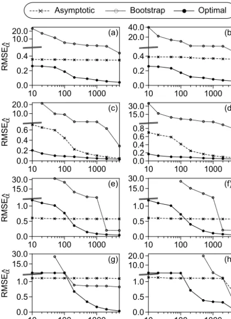
The results (Fig. 1) show that the new optimal order selec-tor outperforms (i.e. has a smaller RMSE
b
α) the two
competi-tors. This is true over a considerable range of design param-eters (n, τ, α). The success of the optimal order selector may at least partly be due to the situation that the normality ofbα, on which the two competing selectors are based, has not been approached in the simulation world. On the other hand, the prescribed stable distributional shape of the data-generating process fits particularly well to the optimal selector (Algo-rithm 1). This point will be investigated in a future analysis of the optimal selector under varied Monte Carlo designs.
4 Error bars
To adapt the preface to our book on climate time se-ries analysis (Mudelsee, 2014): we wish to know the truth about a geophysical system, but have only a limited sam-ple,{t (i), x(i)}n
i=1, influenced by various sources of noise.
Therefore we cannot expect our estimate,bα, which is based on data, to equal the truth. However, we can determine the typical size of that deviation: an error bar. Error bars help to critically assess estimation results, they prevent us from mak-ing overstatements, and they guide us on our way to enhanc-ing geophysical knowledge. Estimates without error bars are useless.
The Monte Carlo experiment (Sect. 3) contains a method to construct error bars. For this purpose, Algorithm 2 may be adapted as follows. Line 1: take overnfrom the sample, and setτ=
bτ andα=bα. Lines 2 to 4: take over{t (i)}
n i=1
10 100 1000 0.0 10.0 20.0 0.2 0.4 RMSE a (a) ^
10 100 1000
0.0 20.0 40.0 0.2 0.4 (b)
10 100 1000
0.0 10.0 20.0 0.2 0.4 0.6 RMSE a (c) ^
10 100 1000
0.0 15.0 30.0 0.2 0.4 0.6 0.8 (d)
10 100 1000
0.0 1.0 15.0 30.0 0.5 RMSE a (e) ^
10 100 1000
0.0 1.0 15.0 30.0 0.5 (f)
10 100 1000
n 0.0 1.0 15.0 30.0 0.5 RMSE a (g) ^
10 100 1000
n 0.0 1.0 10.0 20.0 0.5 (h)
= Asymptotic + Bootstrap , Optimal
Figure 1.RMSE of the estimated heavy tail parameter in depen-dence on data size for the Hill estimator and various order selec-tors: optimal (Algorithm 1), asymptotic normality and bootstrap. The Monte Carlo design parameters are prescribed persistence time,
τ=0.0(a, c, e, g)andτ=0.8(b, d, f, h); prescribed heavy-tail pa-rameter,α=0.5(a, b),α=1.0(c, d),α=1.5(e, f)andα=2.0 (g, h); and number of simulations,nsim=10 000. Note the broken
yaxes.
it includes not only estimation variance, but also bias. This makes it more reliable than, for example, the standard error. This error bar construction is also used for the persistence time (RMSE
b τ).
A note on the selection ofnsim=100 for error bar
determi-nation: we explored the influence ofnsimon the accuracy of
RMSEbα in another Monte Carlo experiment. We variednsim
and analysed the coefficient of variation (CV) of RMSEbα.
The CV is given by the standard deviation of RMSE b α, which
is calculated over a number of external (i.e. outside of the al-gorithm) runs, divided by the mean calculated over the runs. One run consists in generating a series and estimating the tail index with RMSE
bα. The number of runs was 10 000. We found that for a number ofnsim≈100, a saturation behaviour
of the CV sets in, while for smallernsimvalues, the CV
de-creases with nsim. Further increasing nsim had no
measur-able effect on the accuracy of RMSE
bα. The value of 100 also
agrees roughly with the Monte Carlo findings on the min-imum number of simulations required for obtaining reliable results for the bootstrap standard error (Efron and Tibshirani, 1993).
5 Application to artificial time series
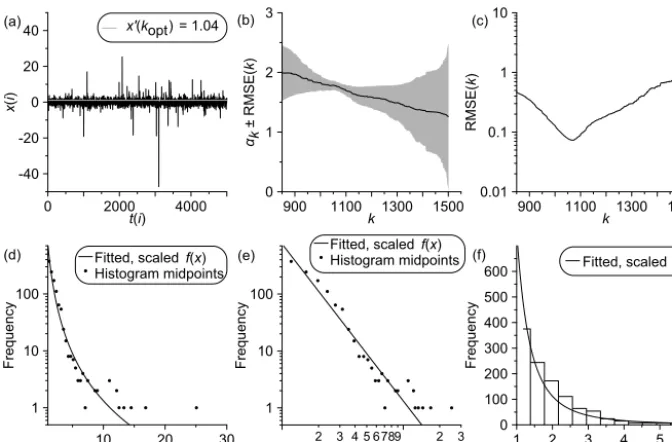
The application of heavy tail estimation to artificial data (Fig. 2) offers a test of the new analysis method because the properties of the data-generating process (τ, α) are pre-scribed and can be compared with the estimates (bτ ,bα). Em-ploying a data size (n=5000) not untypical for ambitious non-linear geophysical analyses and using the new order se-lector yields a clearly expressed optimal order ofkopt=1071
(Fig. 2c). That means about 20 % of the data are utilized for heavy tail index estimation.
It is remarkable that the sequencebαkdoes not at all display
a plateau at aroundkopt(Fig. 2b). Rather, the sequence shows
a trend that decreases withk.
The resulting estimates with RMSE error bars fromnsim=
100 simulations (Sect. 4) agree well with the prescribed val-ues: for the persistence time, τ=1.50 andbτ±RMSE
bτ = 1.46±0.04; for the heavy tail parameter,α=1.75 andbα± RMSE
b
α=1.76±0.06.
The good agreement between data and fit is also reflected by the good agreement between data histograms and fitted densities (Fig. 2d–f).
One caveat to consider is the fact that the prescribed den-sity of the process that generated the data (Fig. 2a) is a stable distribution, which is also employed by optimal order selec-tion (Algorithm 1). This may have, at least partly, produced the good fit on artificial data. On the other hand, (1) the full distribution does not need to follow the distribution, just the extremal part, and (2) stable distributions form a fairly wide class of distributions (Nolan, 2003). Still, we plan to study the relevance of this point by means of an analysis under var-ied Monte Carlo designs.
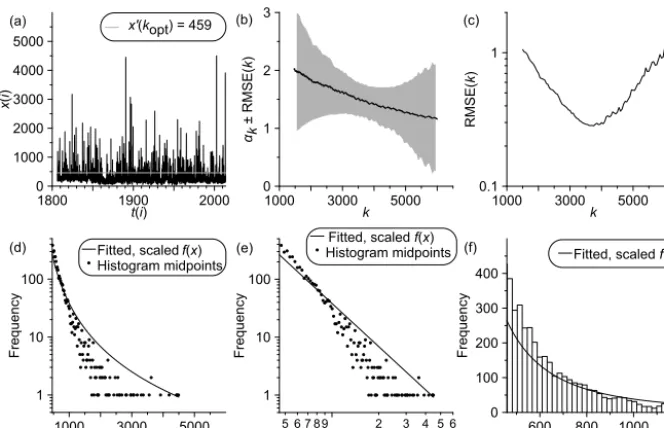
6 Application to observed, hydrological time series The application of heavy tail estimation to observed data (Fig. 3) serves to illustrate the practical work. The runoff time series of the River Elbe at station Dresden (Fig. 3a) belongs to the longest observed hydrological records avail-able. The data quality is assessed as excellent owing to the relatively constant observation situation at this station and the frequently updated runoff–water stage calibration curves (Mudelsee et al., 2003). We analyse the hydrological sum-mer separately (Fig. 3) because the conditions for generat-ing extreme floods (right tail) vary from summer to winter (Mudelsee et al., 2003). The resulting data size isn=38 272. The clearly expressed optimal order for Hill estimation is kopt=3732 (Fig. 3c). This means about 10 % of the data are
0 2000 4000
t(i)
-40 -20 0 20 40
x
(
i
)
900 1100 1300 1500
k
0 1 2 3
k
± RMSE(
k
)
900 1100 1300 1500
k
0.01 0.1 1 10
RMSE(
k
)
1 2 3 4 5 6789x 10 2 3 1
10 100
Frequency
1 2 3 4 5 6
x
0 100 200 300 400 500 600
Frequency
Fitted, scaled f(x)
10 20 30
x
1 10 100
Frequency
Fitted, scaled f(x) Histogram midpoints
x'(kopt) = 1.04
Fitted, scaled f(x) Histogram midpoints
(a) (b) (c)
(f) (e)
(d)
Figure 2.Application of heavy tail estimation with optimal order selection to artificial data:(a)time series (dark line), drawn from an AR(1) process with even spacing unity and stable distributed innovations (n=5000, τ=1.5, α=1.75);(b) sequencebαk (solid dark line)±RMSE(k)(shaded) for the Hill estimator (right tail);(c) measure RMSE(k);(d)–(f) frequency plots showing densities and his-tograms at various axis scalings. The optimal order iskopt=1071. The fitted heavy tail density function,f (x), has been scaled such that for
x > x0(kopt), the tail probability,F (x)(Eq. 1), timesnequals the number of extreme events (right tail). (Note thatRf (x)=F (x).)
ratio kopt/nwithn, which is found when the observed
se-ries is compared with the artificial sese-ries of size n=5000 (Sect. 5), is compatible with theoretical recommendations (Hall, 1982).
Due to excessive computing costs associated with a brute force search forn=38 272, the optimal order is found via a quasi-brute force, two-step search method. In the first step, we calculate the measure RMSE(k) (Algorithm 1) at k -increments ofLk=50. From the resulting 765 measure
val-ues, we selectPmink=5 % with minimal measure, for which
we perform in the second step a fine search with increment 1. The quasi-brute force search, Monte Carlo experiments and further hints on the selection ofLk andPmink are described
in the manual (Supplement).
The resulting estimates with RMSE bars fromnsim=100
simulations arebτ =0.060±0.002 a andbα=1.48±0.13. Al-though the observed time series clearly has more points (n=38 272) than the artificial one (n=5000), the error bar for the heavy tail index estimate is larger (RMSEbα=0.13)
than for the artificial one (RMSEbα=0.06). The reason is
that the estimated “equivalent autocorrelation coefficient” (Mudelsee, 2014), given byba¯=exp(− ¯d/bτ ), is larger for the observed time series (ba¯=0.91) than for the artificial one (ba¯=0.51). Stronger persistence means fewer independent data points and a larger estimation uncertainty. An additional Monte Carlo experiment revealed that for absent persistence (τ =0), the observed, hydrological values yield a clearly smaller error bar (RMSE
b
α=0.03).
For the hydrological interpretation of the statistical results, not only the error bars (RMSE
bτand RMSEbα) have to be con-sidered, but also model mis-specification.
In the case of persistence estimation of runoff series, an al-ternative to the AR(1) model may be a long-memory model (Mudelsee, 2007). We think that the large estimated auto-correlation (ba¯=0.91) does already capture a large amount of the serial dependence structure (Sect. 1) of the hydrolog-ical series. Therefore, an associated persistence model mis-specification would likely have consequences (widened error bars) that are only minor. Still, it is worth studying more sys-tematically long-memory models with heavy tail distributed innovations.
In the case of heavy tail index estimation, we think that the employed stable distribution model class does already cap-ture the true distribution (Fig. 3d–f) quite well owing to the wide range of the stable class (Sect. 1). Therefore, an asso-ciated distribution model mis-specification should not widen the error bars strongly, and the true estimate should not be far away from the estimate,bα=1.48.
1800 1900 2000
t(i)
0 1000 2000 3000 4000 5000
x
(
i
)
1000 3000 5000
k
0 1 2 3
k
± RMSE(
k
)
1000 3000 5000
k
0.1 1
RMSE(
k
)
10009 2 3 4 5 6
8 7 6 5
x
1 10 100
Frequency
600 800 1000 1200
x
0 100 200 300 400
Frequency
Fitted, scaled f(x)
1000 3000 5000
x
1 10 100
Frequency
Fitted, scaled f(x) Histogram midpoints
x'(kopt) = 459
Fitted, scaled f(x) Histogram midpoints
(a) (b) (c)
(f) (e)
(d)
Figure 3.Application of heavy tail estimation with optimal order selection to observed data:(a)time series (dark line) and average daily runoff of the River Elbe at Dresden (Germany) during summer (May to October) from 1 May 1806 to 31 October 2013 (n=38 272); units: m3s−1;(b)sequencebαk (solid dark line)±RMSE(k)(shaded) for the Hill estimator (right tail);(c)measure RMSE(k);(d)–(f)frequency plots showing densities and histograms at various axis scalings (cf. Fig. 2). The optimal order iskopt=3732; it has been detected using
a quasi-brute force search (see text). Data courtesy Wasser- und Schifffahrtsverwaltung des Bundes, provided by the Bundesanstalt für Gewässerkunde (BfG), Koblenz, Germany.
b
α≈3 (i.e. finite variance), in contrast to our finding. Fur-ther stages of the analysis, to be pursued in a future paper, will therefore include (1) a comparison between summer and winter for the runoff series from Dresden; (2) a quantifica-tion of the sensitivity to the removal of an annual cycle; (3) a comparison among various other stations on the River Elbe and (4) a comparison with other rivers, for which long, high-quality runoff records are available. Evidently, an accurate heavy tail estimation technique with optimal order selection is helpful for this purpose.
7 Conclusions
The tail probability, P (X > x), is crucially important for practical risk analysis, for example, the calculation of the ex-pected losses in the reinsurance business. Instead of a Gaus-sian exponential behaviour (light tail), many observed vari-ables from complex networks show a power law (heavy tail). This law (Eq. 1), which is parameterized by means of the heavy tail index,α, allows us to extrapolate the probability into unobserved, extreme data ranges.
The accurate estimation ofαon the basis of observed data is therefore also crucially important. The “Achilles’ heel” of tail index estimation is order selection, that is, to set how many of the largest values to utilize for the estimation. This paper focuses on a new, optimal order selector (Algorithm 1). The superiority of the new selector is demonstrated in a Monte Carlo simulation experiment (Fig. 1).
The new selector is claimed to utilize the data in an op-timum way for performing an estimation. The resulting er-ror bars (RMSE
bα), which are calculated from computing-intensive simulations (Sect. 4), are comparably small. Hence, the new method allows us to study, more accurately than pre-viously possible, various extremal behaviours, such as the spatial dependence ofαin geostatistical applications or the time dependence ofαon long time series. The time depen-dence may shed light on tipping points in complex systems. In particular, changes inαover time may possibly be used to predict the approach of a sudden change in a geophysical variable (e.g. climate).
The data-generating process (AR(1) with stable distributed innovations) achieves “distributional robustness” because the full distribution does not need to follow Eq. (1), just the extremal part. It also achieves “persistence robustness” be-cause Eq. (3) ensures that for many time series (also un-evenly spaced), the persistence dynamics is captured at least to first order. As a result, the presented method is accurate and widely applicable, and it delivers robust results.
estimation (ht) has also implemented the estimation routine following Pickands III (1975).
The application to an observed, hydrological time series (Fig. 3) delivered the intriguing result of infinite variance (but finite mean) (bα=1.48) of the data-generating process. Infinite variance would have serious consequences for many types of statistical estimation to be carried out on hydrolog-ical data. We recommend analysing more, independent hy-drological data to corroborate or refute this finding.
The wider impact of optimal heavy tail estimation may be not only on the application to the area of instrumental envi-ronmental measurements, but also to reconstructed variables from the areas of paleoclimatology (Cronin, 2010), paleo-hydrology (Gasse, 2009) and dendrochronology (D’Arrigo et al., 2011; Gholami et al., 2015). Furthermore, since ex-treme events in hydrology and related fields may also show the duration aspect (e.g. droughts, heatwaves), the estimation should not be restricted to measured or reconstructed vari-ables. Rather, heavy tail index estimation should be a useful tool also for the analysis of index variables (Kürbis et al., 2009).
Code availability. The code (Fortran 90 source, Windows exe-cutable and auxiliary files) and a manual are available at http: //www.climate-risk-analysis.com/software/ht. The manual is also available as a Supplement to the paper.
The Supplement related to this article is available online at https://doi.org/10.5194/npg-24-737-2017-supplement.
Author contributions. MAB wrote the initial software version and carried out the Monte Carlo experiment (Fig. 1). MM completed the software development, carried out the data analyses and prepared the manuscript.
Competing interests. The authors declare that they have no conflict of interest.
Disclaimer. Please see the source code or the manual for the dis-claimer.
Acknowledgements. We thank two anonymous referees for helpful reviews. We thank Mersku Alkio (RBZ Wirtschaft, Kiel, Germany) and Mark M. Meerschaert (Department of Statistics and Prob-ability, Michigan State University, East Lansing, MI, USA) for comments on the draft manuscript. We thank the BfG for supplying us with the Elbe runoff time series. This work is supported by the European Commission via Marie Curie Initial Training Network LINC (project number 289447) under the Seventh Framework
Programme.
Edited by: Jinqiao Duan
Reviewed by: two anonymous referees
References
Anderson, P. L. and Meerschaert, M. M.: Modeling river flows with heavy tails, Water Resour. Res., 34, 2271–2280, 1998.
Barabási, A.-L.: The origin of bursts and heavy tails in human dy-namics, Nature, 435, 207–211, 2005.
Cronin, T. M.: Paleoclimates: Understanding Climate Change Past and Present. Columbia University Press, New York, 441 p., 2010. Danielsson, J., de Haan, L., Peng, L., and de Vries, C. G.: Using a bootstrap method to choose the sample fraction in tail index estimation, J. Multivar. Anal., 76, 226–248, 2001.
D’Arrigo, R., Abram, N., Ummenhofer, C., Palmer, J., and Mudelsee, M.: Reconstructed streamflow for Citarum river, Java, Indonesia: Linkages to tropical climate dynamics, Clim. Dynam., 36, 451–462, 2011.
Efron, B. and Tibshirani, R. J.: An Introduction to the Bootstrap. Chapman and Hall, New York, 436 p., 1993.
Fishman, G. S.: Monte Carlo: Concepts, Algorithms, and Applica-tions, Springer, New York, 698 p., 1996.
Fortran 90: User manual, available at: http://www. climate-risk-analysis.com/software/ht, last access: 1 December 2017.
Gasse, F.: Paleohydrology, in: Encyclopedia of Paleoclimatology and Ancient Environments, edited by: Gornitz, V., Springer, Dor-drecht, 733–738, 2009.
Gholami, V., Chau, K. W., Fadaee, F., Torkaman, J., and Ghaf-fari, A.: Modeling of groundwater level fluctuations using den-drochronology in alluvial aquifers, J. Hydrol., 529, 1060–1069, 2015.
Hall, P.: On some simple estimates of an exponent of regular varia-tion, J. R. Stat. Soc. B, 44, 37–42, 1982.
Helbing, D.: Globally networked risks and how to respond, Nature, 497, 51–59, 2013.
Hill, B. M.: A simple general approach to inference about the tail of a distribution, Ann. Stat., 3, 1163–1174, 1975.
Jongman, B., Hochrainer-Stigler, S., Feyen, L., Aerts, J. C. J. H., Mechler, R., Botzen, W. J. W., Bouwer, L. M., Pflug, G., Rojas, R., and Ward, P. J.: Increasing stress on disaster-risk finance due to large floods, Nat. Clim. Change, 4, 264–268, 2014.
Kürbis, K., Mudelsee, M., Tetzlaff, G., and Brázdil, R.: Trends in extremes of temperature, dew point, and precipitation from long instrumental series from central Europe, Theor. Appl. Climatol., 98, 187–195, 2009.
Malevergne, Y. and Sornette, D.: Extreme Financial Risks: From Dependence to Risk Management. Springer, Berlin, 312 p., 2006. Mantegna, R. N. and Stanley, H. E.: Scaling behaviour in the
dy-namics of an economic index, Nature, 376, 46–49, 1995. Mudelsee, M.: Long memory of rivers from spatial aggregation,
Water Resour. Res., 43, W01202, doi:10.1029/2006WR005721, 2007.
Mudelsee, M., Börngen, M., Tetzlaff, G., and Grünewald, U.: No upward trends in the occurrence of extreme floods in central Eu-rope, Nature, 425, 166–169, 2003.
Nolan, J. P.: Numerical calculation of stable densities and distri-bution functions, Commun. Stat. Stoch. Models, 13, 759–774, 1997.
Nolan, J. P.: Modeling financial data with stable distributions, in: Handbook of Heavy Tailed Distributions in Finance, edited by: Rachev, S. T., Elsevier, Amsterdam, 106–130, 2003.
Pickands III, J.: Statistical inference using extreme order statistics, Ann. Stat., 3, 119–131, 1975.
Resnick, S. I.:, Heavy-Tail Phenomena: Probabilistic and Statistical Modeling, Springer, New York, 404 p., 2007.