www.atmos-meas-tech.net/7/2437/2014/ doi:10.5194/amt-7-2437-2014
© Author(s) 2014. CC Attribution 3.0 License.
Ash plume top height estimation using AATSR
T. H. Virtanen1, P. Kolmonen1, E. Rodríguez1, L. Sogacheva1, A.-M. Sundström2, and G. de Leeuw1,2 1Finnish Meteorological Institute, Erik Palmenin aukio 1, 00560 Helsinki, Finland
2Department of Physics, University of Helsinki, Gustav Hällströmin katu 2a, 00560 Helsinki, Finland Correspondence to: T. H. Virtanen ([email protected])
Received: 17 March 2014 – Published in Atmos. Meas. Tech. Discuss.: 16 April 2014 Revised: 24 June 2014 – Accepted: 1 July 2014 – Published: 8 August 2014
Abstract. An algorithm is presented for the estimation of volcanic ash plume top height using the stereo view of the Advanced Along Track Scanning Radiometer (AATSR) aboard Envisat. The algorithm is based on matching top of the atmosphere (TOA) reflectances and brightness tempera-tures of the nadir and 55◦forward views, and using the result-ing parallax to obtain the height estimate. Various retrieval parameters are discussed in detail, several quality parameters are introduced, and post-processing methods for screening out unreliable data have been developed. The method is com-pared to other satellite observations and in situ data. The pro-posed algorithm is designed to be fully automatic and can be implemented in operational retrieval algorithms. Combined with automated ash detection using the brightness tempera-ture difference between the 11 and 12 µm channels, the algo-rithm allows efficient simultaneous retrieval of the horizontal and vertical dispersion of volcanic ash. A case study on the eruption of the Icelandic volcano Eyjafjallajökull in 2010 is presented.
1 Introduction
Information on the dispersion of volcanic ash is important for air traffic safety, and satellite observations are the only way to obtain near real-time (NRT) information on volcanic ash plumes on regional and global scales. Specialized satellite data products can be used by the airline industry and aviation authorities to avoid flying in areas affected by ash. In addi-tion, the satellite observations are crucial for constraining ash dispersion models used for ash forecasts. While geostation-ary satellites with high temporal resolution are best suited to near real-time ash monitoring, the polar-orbiting satellites can often provide more detailed information. In particular,
the vertical profile of volcanic ash plumes can be studied us-ing satellite-based multiview instruments. Detailed studies of the plume heights of past eruptions can help to understand the ash dispersion phenomena and to improve the dispersion models.
Height estimates based on multi-angle satellite data us-ing stereo matchus-ing techniques have been used for decades. Early work by Hasler (1981) on satellite-based stereo match-ing height estimates employed two geostationary satellites, and required manual matching of a pair of images. Since then, multiview satellite instruments have become available, and automatic image processing techniques have been devel-oped. Prata and Turner (1997) introduced an algorithm for cloud top height estimates using Along Track Scanning Ra-diometer (ATSR) data. Their method is based on maximizing the cross-correlation of nadir and forward views by allowing the forward view to be shifted. Muller et al. (2002) devel-oped stereoscopic image matchers for the Multi-angle Imag-ing SpectroRadiometer (MISR), based on minimizImag-ing the difference between views, and Muller et al. (2007) describe a refined method for ATSR-2 data. Fisher et al. (2013) fur-ther developed these methods using Advanced Along Track Scanning Radiometer (AATSR) data. The MISR height esti-mate methods have been applied to volcanic ash plumes, e.g., by Scollo et al. (2012). Recently, Zakšek et al. (2013) pro-posed a method combining Spinning Enhanced Visible and InfraRed Imager (SEVIRI) and Moderate-resolution Imaging Spectroradiometer (MODIS) data. Ash plume heights have also been studied by Grainger et al. (2013) using AATSR, SEVIRI, and MIPAS (Michelson Interferometer for Passive Atmospheric Sounding) data.
ash concentrations. The satellite-based instruments typically measure only the total aerosol load in an atmospheric col-umn, without information on the aerosol profile or concentra-tion. Information on the cloud thickness is needed in convert-ing the satellite-retrieved column amounts (g m−2) to con-centrations (g m−3). The radiative transfer models often use rough guesses for the height and thickness of the aerosol lay-ers, e.g., a homogeneous layer between 0 and 2 km might be assumed. This is usually adequate in the retrieval of the am-bient aerosol optical depth (AOD) over broad areas with rela-tively low concentrations. The ash plumes, however, are dis-tinct features, forming a high contrast with the background and having highly varying heights in general. Thus, informa-tion on the plume height may be of considerable importance to the ash load retrievals. Information on plume height and thickness that can be directly obtained from the stereo view geometry of AATSR is limited, but nevertheless valuable. Work on combining the AATSR dual view (ADV) aerosol retrieval algorithm (Kolmonen et al., 2013) with the AATSR correlation method (ACM) plume top height algorithm and automated ash detection is in progress. The aim is to simul-taneously acquire information on the horizontal plume posi-tion and ash mass load, in addiposi-tion to the plume height. The ash-specific AOD retrieval will be discussed elsewhere.
In this article we describe an elevated-feature height esti-mation algorithm for AATSR. Although our focus is on vol-canic ash plumes, the method can in principle be used to es-timate cloud top heights (CTH) or the height of any other feature, such as smoke and dust plumes or surface topogra-phy, provided that there is enough contrast in the measured top of atmosphere (TOA) reflectances or brightness tempera-tures. The ACM algorithm is largely based on existing meth-ods. New aspects are that we allow a simultaneous track shift of the forward view, to compensate for across-track wind components. We also introduce and use several quality parameters based on statistical analyses and allow si-multaneous use of multiple correlation window sizes in the retrievals. New post-processing techniques to remove unreli-able data are discussed as well. One of the key advantages in our approach is the automated ash detection using the bright-ness temperature difference method. The plume top heights are calculated for ash-flagged pixels only, making the algo-rithm very efficient in processing large quantities of data.
to AATSR (TIR channels and stereo view), and the method presented here can be applied to SLSTR data.
In Sect. 2, the area-based correlation method algorithm for the estimation of volcanic ash plume top heights is de-scribed. In this method the correlation between brightness temperature data for the two views is optimized by shifting the forward-view data in the along-track direction. In Sect. 3 we show comparison to available remote sensing and in situ data as well as against surface height data. In Sect. 4 we apply the method to the 2010 eruption of Eyjafjallajökull as a test case. Conclusions are given in Sect. 5.
2 Ash plume height estimate
Here we describe the characteristics of the AATSR instru-ment (Sect. 2.1), the ash detection technique (Sect. 2.2), the basic ideas behind the stereo view height estimate method (Sect. 2.3), and the ACM height estimate algorithm (Sect. 2.4). The height estimate results depend on several pa-rameters used in the retrieval; these are discussed in Sect. 2.5. The primary product of ACM is the single-pixel height, cal-culated separately for each ash-flagged pixel. In addition, an averaged (smoothed) height product is provided, where the acceptance of pixels for the average is decided based on cor-relation method quality parameters and on statistical mea-sures. This post-processing is discussed in Sect. 2.6. 2.1 AATSR instrument
at ground level. The plume height causes deviation from this in the direction along the satellite track, and the magnitude of the shift in this direction provides a way to estimate the plume height. Any of the channels can be used for the height estimate. The thermal infrared channels usually provide the highest contrast of the ash plumes with the background, and the 10.85 µm channel is used by ACM by default. The hori-zontal resolution of AATSR is approximately 1 km.
2.2 Ash detection
A volcanic ash plume can be detected using the brightness temperature difference (BTD) between two wavelengths, 11 and 12 µm (Prata, 1989). In a first approximation, the bright-ness temperature difference, BTD=T11−T12, is negative for volcanic-ash-contaminated pixels and positive for most other situations, such as meteorological clouds and clear-sky scenes. The optimal BTD threshold for ash detected is not al-ways exactly 0 and, e.g., water vapor tends to increase BTD, hiding the ash signal (Yu et al., 2002). Also, false alerts can be caused, e.g., by desert dust or arctic haze. Although more detailed methods for ash detection exist for SEVIRI (Prata, 2013; Naeger et al., 2014) and for AIRS (Clarisse et al., 2010), for the purposes of this paper the simple BTD thresh-old method is sufficient.
2.3 Height estimate principle
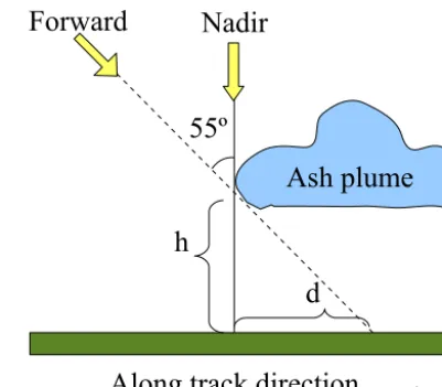
The estimation of the ash plume top height is based on the stereo view of AATSR. The two AATSR views, a near-nadir and a∼55◦forward view, are collocated at ground level. At higher altitudes, the two views are looking at different po-sitions (in the along-track direction), with the difference in-creasing with inin-creasing height. Thus, for an elevated fea-ture with a detectable contrast to the background in both views, the height can be estimated by considering the appar-ent ground level difference in position between the two views (parallax).
A simplified illustration of the geometry is shown in Fig. 1. The cloud seems to be further away (with respect to the ground) in the forward view, as compared to the nadir view. The distance d between the projections of the cloud on the Earth’s surface in the two views gets larger with increasing cloud height h. The simplified picture shows the geometry for sub-satellite track only, for which the nominal nadir and forward-viewing angles are θN=0◦ and θF=55◦, respec-tively, and the height is obtained from h=d/tan 55◦ (see Fig. 1). In the actual conical viewing geometry both viewing angles depend on the position of the pixel along the swath, and the height is obtained fromh=d/(tanθF−tanθN).
The height estimate process is automated by using a cor-relation method. The parallax is obtained by maximizing the correlation between the two views by allowing the for-ward view to be shifted. As a by-product, an estimate for the across-track wind can be obtained by allowing a
two-Nadir
Forward
d
h
Along track direction
Ash plume
55º
Figure 1. Cloud height estimate geometry. The edge of the cloud
(at altitudeh) is observed at different apparent positions at ground level in the two views, with distanced. With increasing height the distance increases.
dimensional shift and taking into account the time gap of approximately 135 s between the two views.
The ACM height estimate is based on the gradients of the measured brightness temperatures (or other quantities) rather than the measured values themselves. If the measured quantities remain constant over large areas, the height can-not be estimated using the stereo view methods. It should also be noted that the total TOA radiation is used in the correlation procedure; for partially transparent plumes or clouds the method might not work. If there are surface fea-tures with high contrast below the plume, they may dominate the correlation.
2.4 Spatial-correlation plume height estimate
1
and white rectangle (b). The forward-view window scans all allowed shifts, and the resulting cross-correlation matrix is shown in panel (c). The maximum value of cross-correlation coefficientCdetermines the best-fitting shift(m, n)selected by the algorithm. In this example, the algorithm picks shift (2, 3) as the maximum correlation shift.
There are various alternative ways to define the cross-correlation coefficient used in automatic height estimation. One of the first methods is described by Prata and Turner (1997) and is based on cross-correlating the measured data, normalized by rms values:
C0(x, y;m, n)= hfN(x, y)fF(x+m, y+n)i
p
hfN(x, y)2ihfF(x+m, y+n)2i
, (1)
wherefN is the measured GBTR value (gridded brightness temperature or reflectance) in the nadir view, andfF is the corresponding value in the forward view, with pixel shift
(m, n)(in along-track (n) and across-track (m) directions). The coordinates x andy refer to the across-track (column) index and along-track (line) index, respectively (not to lati-tude or longilati-tude). Here the averageh. . .iis defined (for both views respectively) as
hf (x, y)i = M
X
i=−M N
X
j=−N
f (x+i, y+j )/Ntot, (2)
where the summation is over the correlation window (CW) andNtotis the total number of pixels in the window. The in-dexiruns through the across-track coordinate and the index
j correspondingly through the along-track coordinate of the CW. The leading idea in the correlation method height esti-mate is then that the highest coefficientC0among all shifts gives the best-fitting pixel shift(m, n), and the correspond-ing height is the most probable plume top height. However, it turns out that using Eq. (1) leads to a lot of noise in the end results. There are many possible reasons for this, including different background atmospheric effects for nadir and for-ward views, and generally noise in the TOA satellite data. It may also happen that there is simply not enough contrast be-tween the plume and the background. Fortunately, there are some statistical tricks to remove part of the background noise and improve the results.
Instead of following the method of Prata and Turner (1997) as such, the approach adopted here is to consider the
deviation of the measured values from the local average, in-stead of the measured values themselves (Muller et al., 2007; Zakšek et al., 2013; Fisher et al., 2013). The cross-correlation coefficientCat point(x, y)between the nadir and forward-view data is defined as
C(m, n)=h(fN−µN)(fF(m, n)−µF(m, n))i
σNσF(m, n)+
, (3)
where the forward view is shifted bympixels in the across-track direction (xaxis) andnpixels in the along-track direc-tion (y axis). Hereis a small constant (0.001 by default) used for numerical stability and to avoid amplification of noise. Here we have dropped the coordinatesxandyfor no-tational brevity. The correlation coefficients are in the range
−1≤C≤1. The averageµN= hfNiis defined as
µN(x, y)=
M
X
i=−M N
X
j=−N
wi,jfN(x+i, y+j ), (4)
where the summation is over the CW of sizeNtot=(2N+ 1)×(2 M+1). The weight factorwi,j can be based on the
distance from the center point(x, y)for weighted average, or simply 1/Ntot for arithmetic average. For the forward-view average, nominally associated with point(x, y)but actually centered at the shifted point(x+m, y+n), we have
µF(x, y, m, n)= M
X
i=−M N
X
j=−N
wi,jfF(x+m+i, y+n+j ). (5)
This means that the whole forward-view correlation window associated with(x, y) is shifted by vector (m, n), as illus-trated in Fig. 2. Naturally, the forward-view average is differ-ent for each shift(m, n). The allowed pixels shiftsmandn
are predefined:m∈ {−Mshift, . . . , Mshift},n∈ {0, . . . , Nshift}; only positive shifts are allowed forn, corresponding to posi-tive heights.
The standard deviationσ is defined as
σN=
q
h(fN−µN)2i, σF=
q
Table 1. Retrieval parameters, which need to be set prior to each
retrieval. The default values are used in the results shown in this paper, unless otherwise indicated.
Abbreviation Description Default
BTD BTD=T11−T12threshold 0 K
CWS Correlation window size 11×11
Nshift Maximum along-track shift 15
±Mshift Maximum across-track shift 5
Channel Channel used in the retrieval T11
for each of the views. The averages are defined as above, with shift(m, n)implicitly assumed for the forward view.
The cross-correlation coefficient is calculated for each pixel(x, y)and for each possible shift(m, n). The shift cor-responding to maximumCis selected as the best-fitting shift for the given pixel (x, y). The height corresponding to this shiftnis then calculated using appropriate satellite–Earth ge-ometry. Ifφ1andλ1correspond to the latitude and longitude of the original point(x, y)andφ2andλ2correspond to the shifted point(x, y+n)(only along-track shiftnis considered in the height estimate), the along-track distanced between these points can be approximated by
d=
q
[cosφ1(λ1−λ2)]2+(φ1−φ2)2Re, (7) whereRe=6371.0 km is the mean Earth radius. The pseudo-Cartesian formula is adequate since we consider only short distances. The height is then obtained from
h= d
tanθF−tanθN
. (8)
The ACM height retrieval algorithm was written in Fortran and implemented as a part of the larger ADV/ASV aerosol re-trieval algorithm. A typical run on an AATSR scene of 10 000 ash-flagged pixels takes about 5 min on a regular desktop computer. A full scene height estimate takes much longer, so the automated ash detection is crucial for NRT volcano monitoring, as discussed in the introduction.
2.5 Retrieval parameters
The ACM height estimate algorithm uses several parame-ters, which affect the results. These include the size of the correlation window, the maximum allowed shifts for the for-ward view (both along-track and across-track, in pixels), the BTD threshold used for ash detection, and the channel used in the correlation method. The primary retrieval parameters are listed in Table 1.
2.5.1 Brightness temperature difference
As already discussed, the threshold BTD<0 K used for ash detection is not necessarily the optimal value for all cases.
Water vapor in the atmosphere increases the BTD, and thus a limit that is too low may cause some ash-contaminated ar-eas to be missed. On the other hand, some phenomena, like arctic haze, may cause small negative BTD values and cause false alerts. For consistency, the threshold of 0 K is system-atically used in this study.
In addition to the initial ash detection, the way in which the ash mask is used in the retrieval affects the results, particu-larly near the plume edges. The ash flags can be used in the correlation window: if a pixel in the window has its ash flag down, it may or may not be taken into account. If pixels from outside the plume are included, the resulting height may be lower than if non-ash pixels are excluded. On the other hand, if only ash-flagged pixels are used in the correlation window, there may not be enough data for reliable results near the plume edges. In the present approach, the non-ash pixels are included in the correlation window.
2.5.2 Wavelength
The height estimate results depend on the choice of the chan-nel used in the correlation method. In Fig. 3 we show full scene height estimates for two different channels – 555 nm and 10.85 µm. The scene consists of an ash plume at 63◦N, 18◦W, extending to southeast, and high-altitude meteorolog-ical clouds in the northern part, and open ocean and low-level clouds. The 10.85 µm channel is more sensitive to the water clouds, and the height estimate shows large elevated features in the northern part of the test scene. In particular, large parts of the water clouds on the northern part of the scene seem to lack sufficient contrast for the visible channel. The visible wavelength channel seems to detect only the thickest parts of the clouds and gives a lower average height for the scene. The average height (standard deviation) is 2.71 (2.2) km for 10.85 µm, and 2.06 (2.1) km for 555 nm. Both channels de-tect heights of 5–7 km for the ash plume, but the shape and other details differ.
Results obtained with the 12 µm channel are similar to those obtained with the 10.85 µm channel (not shown). The thermal channel centered on 10.85 µm (T11) seems to be more sensitive to the ash plumes. For the results shown in this paper, the 10.85 µm channel has been used.
2.5.3 Correlation window size
Figure 3. Effect of wavelength on a full-scene height retrieval. The height maps show the ACM single-pixel height estimates (km a.s.l.) for
an Eyjafjallajökull ash plume and its surroundings on 16 May 2010, obtained at two wavelengths, namely 10.85 µm and 555 nm. The height histograms below the maps show number of pixels within each height bin. See text for details.
Figure 4. AATSR height estimate with three different CW sizes: 5×5, 9×9, and 13×13.The average height for the full scene varies in the range of 2.6–4.1 km for all CWS but settles at∼2.6 km when CWS is increased. Also, the standard deviation of height decreases with increasing CWS. The height histograms below the height maps show how the fraction of high-altitude pixels decreases with increasing CWS.
CWS leads to lower average plume heights, presumably due to the contribution from the lower-level features surrounding the plume.
The default CWS in ACM is 11×11 pixels, but the al-gorithm simultaneously calculates two ancillary height esti-mates with smaller CWS – 9×9 and 7×7. As output, the algorithm provides the height estimates for all three CWS and the standard deviation of the height between them. Cur-rently, the algorithm uses rectangular correlation windows and simple weights wi,j =1/Ntot in the correlation proce-dure, Eq. (4).
2.5.4 Allowed pixel shifts
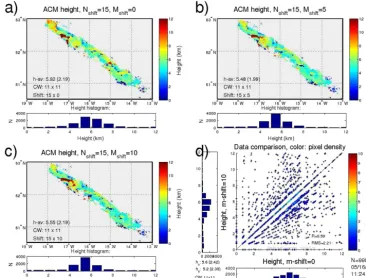
The forward-view correlation window is allowed to shift by m pixels in the across-track direction, and by n pixels in the along-track direction. The shifts are limited by con-ditionsm∈ {−Mshift, Mshift}andn∈ {0, Nshift}. The along-track shift is limited to positive values, corresponding to pos-itive heights. Increasing the maximum allowed shift,Nshift, leads to an increase in the maximum height possible to ob-tain by the algorithm. A large enoughNshiftmust be used so that the largest possible heights can be estimated reliably.
Us-ing unnecessarily largeNshiftincreases computation time and may also result in erroneous, unrealistically high values. Ex-treme along-track shifts can be removed in post-processing. In this work, we useNshift=15, which corresponds to a max-imum height of approximately 12 km. Figure 5 shows how increasingNshiftaffects the results.
The across-track shift does not directly affect the height, but it is important in adjusting to the temporal changes in the image pair and to possible errors in the initial AATSR collocation. From Fig. 6 we see that if the across-track shift is not allowed, the height results would be very different. In this work, the across-track shift is limited byMshift=5, which corresponds to maximum across-track wind compo-nents of approximately 40 m s−1. For comparison, Zakšek et al. (2013) report a maximum column shift of 20 pixels be-tween two SEVIRI images, corresponding to approximately 22 m s−1.
2.6 Post-processing
Figure 5. Effect of the maximum allowed along-track shift,Nshift(orN). Color scale is limited to 0− −9 km although larger heights are
possible, as seen in the height histograms (at the bottom of the figures). We see that most of the changes appear for the highest parts of the plume (as expected), but the scatterplot indicates other differences as well.
effects related to the different viewing angles and the time development of atmospheric features between the observa-tions. To obtain more consistent results, we can use averag-ing over several pixels and statistical filteraverag-ing. The ACM al-gorithm produces data on two levels: first, an SPH estimate is made for each ash-flagged pixel; then, a moving average is calculated for each ash-flagged pixel, using the SPH values of neighboring pixels. Only ash-flagged pixels are considered in the calculation of the average, and quality filters can also be applied before averaging. At the same time, we can calcu-late statistical variables recalcu-lated to the moving averaging win-dow (MAW) and use those for further filtering. The resulting “best average height” (BAV) values are expected to be more representative than SPH data. However, the SPH data is also useful, since the quality filters often tend to remove a large portion of the original pixels.
Naturally, the average height results depend on the MAW size, possible weighting used in the averaging, and on the quality filters. In this section the effects of various parameters are discussed. The filtering parameters are listed in Table 2. Of course, the effectiveness of these parameters in improving the results can only be determined when reliable validation data is available. However, some conclusions can be made based on the variability of the heights; we expect the plume
Table 2. Parameters that can be used for filtering the height estimate
data and the default values. In the ACM output, both the original un-filtered single-pixel heights and the un-filtered MAW-averaged heights are given. See text for details.
Default
Parameter Usage threshold
C C > Clim 0.5
σc σc> σclim 0.15
σCWS σCWS< σCWSlim 20
σav σav< σavlim 3.0
σm σm< σmlim 3
nav n > nav 4
Extrema on/off On
Shadow on/off On
Cloud on/off On
top heights to be rather uniform on horizontal scales of 10 km or so.
Figure 6. Effect of the maximum allowed across-track shift,Mshift(orM), is much larger than that ofNshift. However, the difference between
M=5 andM=10, for example, is already much smaller (R=0.89, not shown) than betweenM=0 andM=10, shown here (R=0.59).
parameters – standard deviation of height within the MAW
σav; the standard deviation of the across-track shift within the MAW, σm; and the number of acceptable pixelsnav within the MAW – are related to the averaging. The three masks that can be applied to the SPH data are used to remove pixels where the algorithm chooses the maximum or zero along-track shift (extrema mask), pixels contaminated by water or ice clouds (cloud mask), or pixels where the forward view may be obstructed by a high feature earlier on the satellite track (shadow mask).
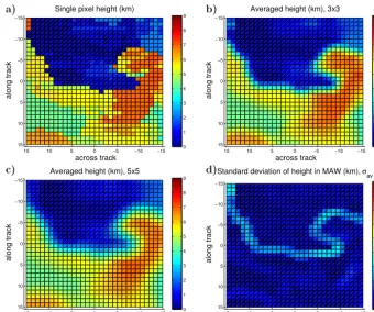
2.6.1 Averaging window size
In principle, there are two ways to do the averaging: increas-ing the pixel size or usincreas-ing the MAW technique. The former would reduce the computational load, but is less flexible, so the latter method is used in the ACM algorithm. The aver-aged height is given in full resolution, i.e., a separate value is calculated for each pixel. Although technically the resolu-tion remains the same, the averaging blurs the details, as seen in Fig. 7. With an increasing MAW size the heights become more uniform but less detailed.
Since the height estimate is based on integer pixel shifts in the along-track direction, the resulting data is quantized, i.e., the height distribution consists of a small number of dis-tinct heights. This is partially smoothed when the pixel shifts are converted to heights, since the height depends on the
lat-itude and on the position along the satellite swath. The av-eraging further smooths the data, hiding the initial quantized nature of the retrieval. Figure 7 illustrates the smoothing us-ing a movus-ing averagus-ing window.
When calculating the average heights, the standard devia-tions of height (σav) and across-track shift (σm) within the
MAW are also calculated. As discussed above, only ash-flagged pixels are used in the averaging, and some of the ash-flagged pixels within the MAW may be removed before the averaging by applying various thresholds. The number of acceptable pixels used in the average (nav) is recorded. 2.6.2 Cloud screening
−15 −10 −5 0 5 10 15 −15 −10 −5 0 5 10 15 across track along track
Single pixel height (km)
0 1 2 3 4 5 6 7 8 9 a) −15 −10 −5 0 5 10 15 −15 −10 −5 0 5 10 15 across track along track
Averaged height (km), 3x3
0 1 2 3 4 5 6 7 8 9 b) −15 −10 −5 0 5 10 15 −15 −10 −5 0 5 10 15 across track along track
Averaged height (km), 5x5
0 1 2 3 4 5 6 7 8 9 c) −15 −10 −5 0 5 10 15 −15 −10 −5 0 5 10 15 across track along track
Standard deviation of height in MAW (km), σ
av 0 1 2 3 4 5 6 7 8 9 d) 1
Figure 7. The effect of the averaging with a moving averaging window (MAW). (a) The initial single-pixel heights; (b) the MAW size 3×3 averaged values; (c) the MAW size 5×5 values. The averaging smooths the data, removing isolated peaks, but some details are lost. (d) The standard deviation of height within the MAW clearly indicates the plume edges.
in aerosol retrieval cannot be used in ash-specific retrievals, since they tend to misidentify ash plumes as clouds. How-ever, assuming that the water/ice clouds are brighter than the ash plumes, we can use a reflectance test at 659 nm to re-move ash-flagged pixels with possible cloud contamination. The cloud test analyses one AATSR scene and automatically determines a reflectance threshold, above which the pixel is flagged as cloudy (González, 2003). Figure 8 shows the ef-fect of cloud mask on a test case. The false-color image of the scene (not shown) shows a water cloud layer below the ash plume around the central and southern parts of the plume.
The cloud mask can be applied to the data before averag-ing, but for many cases it is too stringent and removes most of the ash-flagged pixels. For the Eyjafjallajökull eruption the cloud mask removes on average more than 50 % of the ash-flagged pixels. The effect of the cloud screening is case dependent, and manual inspection of the images is often re-quired for optimal results.
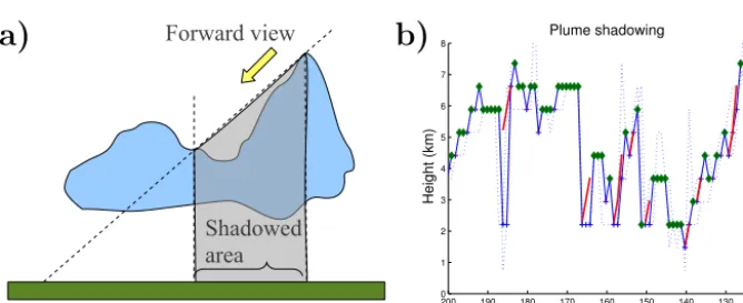
2.6.3 Shadow screening
At a given position along the satellite track, the forward view may be blocked by high plumes earlier on the track. The high features cast a “shadow”, the height of which decreases with distance. If the height of the “shadow” is higher than the height estimate given by the algorithm, the pixel is masked
as “shadowed” (Fig. 9). The shadow mask is calculated from the initial single-pixel height estimates. For the Eyjafjalla-jökull eruption, the shadow mask typically removes 10–30 % of the initial pixels.
2.7 Error characterization
Several assumptions are made in the height estimate method, and there are numerous sources of error. It is difficult to accurately quantify all the various error sources due to the nature of the correlation method. However, the quality pa-rameters introduced in the previous section can be used to asses the contributions from different error sources to the height estimate.
2.7.1 Resolution
Figure 8. Eyjafjallajökull eruption 15 May 2010. We show the effect of removing the ash pixels flagged as cloudy by 659 nm reflectance
cloud test. In panel (a) we show all SPH values, while in panel (b) the cloud-flagged pixels have been removed. The average height decreases from 2.40 to 2.29 km when the clouds are removed, but the height histograms (below the maps) show that there are no dramatic changes in the height distribution.
Forward view
Shadowed area
Along track direction
a)
120 130 140 150 160 170 180 190 200 0 1 2 3 4 5 6 7 8
Distance from ref. point (km)
Height (km)
Plume shadowing
b)
Figure 9. (a) Principle of the plume shadowing. A high feature can block the forward view (for lower features) in the along-track direction.
A reliable height estimate cannot be obtained for pixels in the shadowed area. (b) An example of shadow masking, an along-track height profile. The blue line shows the initial height estimate. The high features block the forward view on the areas indicated by the red lines, preventing the height estimate. The green dots indicate heights accepted after the shadow masking. Note that in the shadowed areas the method typically suggests uniform, underestimated heights.
(Sect. 3.1). In addition, there are several error sources that may have a more significant contribution to the total error. These are discussed in more detail below.
The horizontal resolution (pixel size) is approximately 1 km, with the exact value depending on latitude and on the position along the swath. The algorithm output contains height estimates in the full resolution. A moving average value over 25 (by default) neighboring pixels is also provided for each pixel, with the same nominal resolution.
2.7.2 Correlation method quality
The quality of the correlation method height estimate can be assessed using several quantities. First, the correlation coef-ficientC of each pixel is a natural measure of the quality of the estimate: for pixels withCapproaching 1, we have high confidence in the reliability of the estimate, while pixels with
C <0.5 are removed by default filters. (By “correlation co-efficient of a pixel” we mean the maximum cross-correlation
coefficient over all possible shifts for the CW centered on the said pixel.) Low values ofCmay occur due to many rea-sons. Large changes in the plume shape and position in the approximately 130 s time gap between the views is one pos-sible cause for a lowC value. Poor correlation can also be caused by effects due to differences in the viewing geom-etry; the forward view has a longer light path and is more affected by an ash layer. Also the underlying surface texture may have different relative contributions in the two views.
The second parameter that can be used in quality assess-ment is the standard deviation of the correlation coefficient,
Figure 10. (a) Topographic data over the Himalayas, (b) AATSR height estimate, (c) their difference, (d) the across-track pixel shift, (e)
a crosscut height profile, and (f) the scatterplot for topographic height and ACM estimate. Some cloud contamination can be seen in the ACM height estimate, particularly on the southern edge of the mountain range. These cause the largest differences, seen as the red areas in panel (c), narrow peaks in panel (e), and as large scatter in panel (f). The crosscut is indicated in panel (b) as the dashed red line. The vertical resolution of roughly 1 km is clearly seen in the height estimate profile (e), as well as the jumping of the algorithm between 0 and 1 km in the lower plains. Panel (d) shows features resembling the conical scanning geometry of AATSR and may indicate ground level collocation errors.
whereσcmight be low is glinting sea surface, where any de-tectable features may be hidden in the noise.
2.7.3 Multilayer structures and transparency
Errors due to multilayer structures and transparent ash plumes are particularly difficult to quantify. The height esti-mate algorithm provides the height of the dominating feature in the scene, which may not necessarily be the ash plume but, e.g., an underlying water cloud or the ground surface. The correlation method relies on the assumption that the detected ash plume is the dominating feature in the scene so that the algorithm can reliably track and collocate the plume features. However, if the ash plume is thin and transparent, the un-derlying surface texture may dominate the cross-correlation. Thus the algorithm may not always find the plume top height but the height of some other feature.
The noise seen in the initial SPH data may be partly due to the algorithm jumping between the plume top level and surface- or cloud-level collocation. The variation of SPH within the MAW or between different CWS can be used as indicators of such jumping between features at different heights. The algorithm attempts to minimize the occurrence of such cases by applying thresholds toσavandσcws.
2.7.4 Collocation
The across-track shift obtained as a by-product in the height retrieval can be used as a qualitative indicator of pos-sible errors due to along-track wind, if further information on the wind direction is available. As an example, a rough esti-mate of the wind speed can be made from Fig. 6. For the ash plume (BTD<0) the average across-track shift is 1.5 pixels (not shown), corresponding roughly to 11 m s−1wind speed. From the direction of the ash plume relative to the swath, we can estimate that the along-track component is roughly one-third of this, i.e., smaller than 4 m s−1. This corresponds to an along-track shift of less than a pixel, and thus it is not likely that the along-track wind causes very large error in the height estimate in this case. In general, if we assume the along- and track wind components to be equal, the typical across-track shift of one pixel indicates an uncertainty of∼1 km in the height.
The ash plume may also change its shape and altitude be-tween the two observations. Prata and Turner (1997) argue that the vertical updraft as such is not a major source of er-ror, since the height information is essentially obtained at the time of the forward overpass. Also, since the correlation win-dow size is typically on the order of 10 km2, modest changes in the cloud morphology should not have a large effect on the height estimate.
3 Validation and comparisons
The height estimates should be validated against indepen-dent in situ sources and compared to available remote sensing data. In this section we compare the ACM height estimates to five independent sources. Since the algorithm can be used to estimate the height of any elevated feature, including ground surface, we can verify the method principle against surface topography data. We also use two satellite-based instruments, MISR and CALIOP, for comparison. In addition, we use data from two ground-based sources for the Eyjafjallajökull erup-tion, the Keflavík weather radar, and a database derived from web camera imagery.
3.1 Topography
Comparison against topographic data is the best way to vali-date the principle of the algorithm. Accurate information on
ever, the overwhelming availability and quality of the topo-graphic data is valuable for testing the basic principles of the height estimate method.
For this test case we have chosen an almost cloud-free scene over the Himalayas on 4 May 2010 at 04:19 (all times in this article are given in UTC), AATSR orbit ATS_TOA_1PRUPA20100504_041906. The surface heights are obtained from http://topex.ucsd.edu/cgi-bin/get_ data.cgi/. The area has sufficient contrast in both surface re-flectivity and brightness temperatures for the tests to work in principle: the mountain tops are cold and snow covered, while the surrounding terrain has darker surfaces and higher temperatures. Although we searched for least possible cloud cover, some uncertainty is still caused by cloud contamina-tion. The difficulty is that the standard cloud tests mask the mountain tops as cloudy, since they are bright and cold, and it is difficult to distinguish between the actual clouds (which are an inconvenience here) and the mountain tops (which we are studying).
Table 3. Number of the common pixels (N) for the MPHP and ACM data, the corresponding average heights for the full original plumes (orig) and for common pixels only (comm), and the corre-lation coefficientR. Only the SPH values for ACM are shown here.
Date N horigacm horigmphp hcommacm hcommmphp R
15 Apr 2856 4.63 2.43 5.67 2.66 0.21 18 Apr 1008 2.30 1.81 3.52 2.16 −0.31 19 Apr 3285 1.77 0.94 1.81 1.32 −0.08 03 May 525 5.04 3.69 5.97 3.79 −0.36 7 May 3814 3.08 3.88 3.16 3.28 0.53 12 May 1188 4.86 5.26 4.25 5.26 −0.20 13 May 13 741 3.55 2.62 3.32 2.57 0.12 16 May 2995 5.45 6.13 5.53 6.06 0.19
3.2 MISR
MISR, with its nine views, is an optimal instrument for height estimates of atmospheric features. Unfortunately, for our purposes it has limited usability due to its lack of TIR channels for ash detection. However, it provides useful com-parison data for the ACM height estimates. There are a num-ber of M-series height estimate algorithms and various tools for cloud top height estimates (Muller et al., 2002, 2007; Fisher et al., 2013). A useful tool for analyzing the plume properties using MISR data, the MISR INteractive eXplorer (MINX), is available as open-source software (Nelson et al., 2013). MINX offers better resolution than the operational MISR product, but requires manual detection of the ash plumes. Plume top heights obtained with MINX have been compared with thermal height estimates and ground-based radar results by Ekstrand et al. (2013). Particularly interest-ing for our work is the MISR Plume Height Project (NASA, 2013), where the height estimates are calculated for some manually selected ash plumes. In the following we compare the height estimates made with the ACM to the MISR Plume Height Project (MPHP) height estimates.
In Table 3 we show the average heights for both AATSR and MISR data for the eight cases where overlapping data ex-ists. In the comparison only common pixels have been used, i.e., data is limited by both the MPHP handmade plume poly-gon and by the AATSR BTD<0 K threshold. We have used the MPHP grid, and averaged the ACM data within a 4 km radius from the grid point. The number of common MPHP pixelsN is given in the table. The pixel-by-pixel correlation coefficientsR are also given for each case, and we see that the correlation is poor. This is not surprising, given that there is a time gap of approximately 2 h between the overpasses, during which the plumes may have shifted. The averaged plume heights are a better starting point for the comparison, but some collocation and ash identification issues remain. For example, the common pixels (those that pass the AATSR BTD<0 K thresholds and are within the MPHP polygon) may not give representative subsets of the plume height data.
A more reasonable comparison might be achieved by manu-ally selecting corresponding plume areas from both data, tak-ing into account the horizontal motion of the plume durtak-ing the time lapse, but such selection is prone to interpretation bias and is not conducted here.
The heights averaged over common pixels are similar for all cases, except the first one on 15 April. For this case, the MPHP plume polygon is not strictly limited to the ash plume, but contains surrounding sea surface areas as well. This is seen as the much smaller average height than for ACM in the comparison.
In Fig. 11 we show MPHP and ACM data, and their com-parison, for an Eyjafjallajökull ash plume just south of Ice-land on 16 May 2010. For AATSR, we use the SPHs; com-parison with the BAV data gives only slightly improved re-sults. For the test case data, limited by both the MPHP plume area and by the AATSR BTD threshold, the aver-age height (standard deviation) is 6.1 (0.57) km for MPHP and 5.5 (1.15) km for ACM. Although the heights averaged over the whole plume are not too different, the pixel-by-pixel scatterplot shows poor agreement. Part of this can be ex-plained by the∼2 h time gap between the overpasses; from the false-color image (not shown) we can clearly see that the plume has shifted to the north between the AATSR and MISR images, which is not taken into account in the scatterplot. We see that the MISR results show rather uniform heights, whereas much more variation is seen in the AATSR data.
There are several differences in acquisition of the two data sets. Although the correlation algorithms are based on the same principles, there are differences in the normalization procedures, correlation window sizes, and other retrieval pa-rameters. The MPHP data is obtained using a visible wave-length channel (671 nm), while for AATSR we use a TIR channel (10.85 µm). Also, for the MISR data smaller view-ing zenith angles (VZA) are used: MPHP typically uses six of the oblique cameras, labeled A (26.1◦), B (45.6◦) and C (60.0◦), paired with the nadir view camera for in the correla-tion method. A lower VZA leads to lower vertical resolucorrela-tion, and thus to more uniform plume heights for MPHP data. On the other hand, a larger VZA leads to increasing differences in the viewing geometry and increasing errors due to plume shadowing and different light path lengths. There are wind-corrected height estimates available for the MISR data, but in the comparison we have used only data without wind cor-rection.
Figure 11. The MPHP and ACM (SPH) plume heights and their difference, limited by both the MPHP plume and AATSR-detected ash plume
(BTD<0 K). AATSR gives 0.5 km lower heights on average, with significantly more variation (σh=0.6 km for MISR andσh=1.2 km for AATSR), as can be seen from the height histograms (below the height maps). The differences are centered roughly on 0, but the scatterplot shows poor pixel-by-pixel correlation (R=0.2) between the instruments.
3.3 CALIOP
The lidar data from the CALIOP on the Cloud–Aerosol Lidar and Infrared Pathfinder Satellite Observations (CALIPSO) platform (Winker et al., 2007) gives accurate ash plume heights, but with its limited coverage it is difficult to find even remotely simultaneous overpasses with AATSR, where ash is present. One such case is found southwest of Iceland, where a large ash cloud is observed by AATSR on 7 May 2010 at 22:51. The plume is crossed by CALIPSO some 5 h later on 8 May 2010 at 04:04. From hourly SEVIRI data (Prata and Prata, 2012; Prata, 2013) between 23:00 7 May and 04:00 8 May we see that the ash plume, which initially coincides with the plume observed by AATSR, moves south by approx-imately 2◦in 5 h (Fig. 12). Considering this, there is remark-able agreement between the ACM height estimate and the CALIOP sounding.
The CALIOP data shows three thicker ash layers approx-imately at 10, 7.5, and 5 km heights, and ACM shows data at similar altitudes. There are also lower-level cloud struc-tures at ∼3 and ∼1 km levels, which are picked out by ACM at the edges of the plume. It is possible that the ver-tical structure of the plume is changed in the 5 h between the observations, but the smooth transition of the plume with only modest changes in the horizontal shape (as observed in
the six SEVIRI images acquired hourly) imply that drastic changes have not necessarily occurred. A few other similar cases of near simultaneous overpasses can be found, with de-cent agreement between the data but with some collocation issues remaining.
3.4 Weather radar and webcam
Figure 12. Eyjafjallajökull eruption, 7–8 May 2010; a near-simultaneous overpass of AATSR and CALIPSO over a large ash cloud. (a) The
shaded blue area shows the AATSR swath on 7 May at approximately 22:51, while the red line shows the CALIPSO track on 8 May at approximately 04:05. The color-coded pixels show the ACM height estimate. The yellow area shows ash plume detected by SEVIRI on 7 May at 23:00, which coincides with the ACM plume (within the AATSR swath). The orange area shows the plume observed by SEVIRI 5 h later, at the time of CALIPSO overpass. (b) CALIOP backscatter profile on 8 May at 04:00, with the ACM height estimates from 7 May 22:51 shown by the red symbols. The ash plume is seen between 46 and 48◦N in the back scatter data, while for ACM it was observed near 48–49◦N.
17/04 22/04 27/04 02/05 07/05 12/05 17/05 22/05 0
2 4 6 8 10
Date
Height (km)
Average plume top heights, km asl
Radar Webcam ACM
Figure 13. Ground-based plume top height data for the
Eyjafjal-lajökull plume from the Keflavík weather radar and a web camera at Hvolsvöllur (Arason et al., 2011), combined with the AATSR height estimates near the volcano. The radar data is limited from below by 2.5 km and the web camera data is limited from above to 5.2 km (dashed black lines). The ACM data is an average over all ash-flagged single-pixel heights within 50 km from the volcano (both day- and nighttime data).
4 Case study: Eyjafjallajökull
As an example, we apply the AATSR correlation method height estimate algorithm to the Icelandic Eyjafjallajökull eruption in 2010. The course of eruption and ash dispersal is described, e.g., by Gudmundsson et al. (2012). Ash de-tection and mass load retrieval by SEVIRI for the eruption period is described by Prata and Prata (2012), and a detailed dispersion model study, including plume height information, is presented by Stohl et al. (2011). Ash identification and re-trieval of ash properties using MISR are described by Kahn and Limbacher (2012). Volcanic ash plume top heights for several days in April during the eruption are estimated using combined SEVIRI and MODIS data by Zakšek et al. (2013). The eruption can be divided into three periods: in the first phase (14–17 April) ash was spread to the southeast over northern and central Europe; in the second phase (18 April– 4 May) less ash was produced and it was only observed near Iceland; in the third phase (5–18 May) the eruption intensity increased again, and ash was dispersed in all directions and over large distances.
Figure 14. Single-pixel height for selected plumes on 4 days in May 2010. The yellow shaded areas show the AATSR swath, with the blue
numbers giving the UTC time of the orbit. The color-coded pixels give the ACM height estimate (km a.s.l.). The text inserts in the lower left show the average height (standard deviation) and the number of pixelsNin each image.
the detection with the 0 K threshold. In the third phase of the eruption, we observe several large ash plumes and clouds in all directions around Iceland. In Fig. 14 we show the height estimate for 4 days during the latter part of the eruption. The figure also illustrates the typical AATSR swaths near Ice-land; the AATSR revisit time is approximately 3 days, and even large plumes may be missed in the gaps between the orbits.
Using the BTD<0 K threshold, we have searched for day-time ash plumes in the period from 15 April to 18 May 2010, in an area between 40◦W, 35◦E and 40◦N, 80◦N. Ash was detected on 25 AATSR orbits for 17 different days. In night-time retrievals, 18 additional ash-affected orbits were found, on 15 different days. Days where the 0 K threshold showed only a limited number of isolated ash-flagged pixels were in-terpreted as false alerts and removed from the analysis. Al-though some clouds detected by the 0 K threshold may be false alerts, like the low-level cloud over Greenland on 6 May seen in Fig. 14a, all ash-flagged pixels are included in the analysis for the days considered for consistency.
17/04 22/04 27/04 02/05 07/05 12/05 17/05 0
1 2 3 4 5 6 7 8 9 10
Date
Height (km)
Time series, Height (km)
Best av. height Single pixel height
a)
17/04 22/04 27/04 02/05 07/05 12/05 17/05 0
5 10 15x 10
4
Date
Number of ash pixels
Time series, Number of ash pixels
All pixels Best av. pixels Clouded pixels Shadowed pixels Extreme shifts
b)
1
Figure 15. Time series of daily average heights and number of ash pixels. The blue lines give the average values using all pixels (SPH),
and the red lines give average values using the filtered pixels only (BAV). The dotted blue lines on the left show the error bars (standard deviation). On the right we also show the number of pixels flagged as clouded or shadowed and also the number of pixels with an extreme (maximum or zero) along-track pixel shift.
Table 4. Daily average heights (standard deviations) for the Eyjafjallajökull eruption and mask fractions for daytime orbits.Nis the number of pixels with a valid height estimate, and bav frac. gives the fraction of filtered (best-average-height) pixels. The other fractions give the portion of pixels flagged by the cloud and shadow masks. In addition to the best average heights (BAV) and single-pixel heights (SPH) calculated with the largest correlation window size (CWS 11×11), we show the single-pixel height calculated simultaneously with two smaller correlation window sizes; the medium window height (MwH, 9×9) and the small window height (SwH, 7×7). Heights are given in kilometers a.s.l.
Date N Bav frac. Cld frac. Shd frac. BAV SPH MwH SwH
15 Apr 11 641 24.0 % 43.3 % 28.2 % 5.03 (3.1) 3.84 (3.5) 4.08 (3.6) 4.52 (3.8)
16 Apr 7333 0.9 % 97.4 % 26.2 % 1.41 (1.1) 4.17 (3.9) 4.48 (4.0) 4.93 (4.1)
17 Apr 14 529 48.0 % 4.9 % 12.1 % 1.96 (1.0) 1.59 (1.6) 1.84 (2.1) 2.47 (2.9)
4 May 4431 10.5 % 65.1 % 12.6 % 1.14 (0.3) 2.58 (3.2) 2.87 (3.6) 3.44 (3.9)
6 May 57 360 26.0 % 64.4 % 11.7 % 3.09 (1.5) 4.70 (2.3) 4.72 (2.4) 4.86 (2.7)
7 May 132 809 8.2 % 83.1 % 30.8 % 2.81 (1.9) 4.36 (3.4) 4.57 (3.5) 4.87 (3.7)
8 May 86 780 25.7 % 46.9 % 35.1 % 2.03 (1.9) 3.28 (3.3) 3.64 (3.6) 4.17 (3.9)
9 May 103 825 25.6 % 19.0 % 23.7 % 2.64 (2.4) 2.13 (3.0) 2.50 (3.3) 3.11 (3.6)
10 May 26 400 19.7 % 47.0 % 21.1 % 2.58 (2.0) 2.24 (2.9) 2.65 (3.2) 3.26 (3.5)
11 May 5418 40.8 % 27.6 % 18.7 % 3.78 (1.7) 3.14 (2.1) 3.41 (2.4) 3.80 (2.9)
12 May 8801 20.4 % 69.2 % 16.6 % 4.53 (1.6) 4.28 (1.9) 4.37 (2.1) 4.56 (2.4)
13 May 69 639 39.3 % 37.7 % 23.8 % 3.97 (1.4) 4.23 (2.2) 4.42 (2.5) 4.77 (2.9)
14 May 51 443 32.2 % 42.7 % 24.0 % 3.96 (2.2) 3.85 (2.7) 4.06 (2.9) 4.44 (3.2)
15 May 65 697 33.0 % 28.5 % 21.5 % 2.81 (1.9) 2.37 (2.5) 2.69 (2.8) 3.23 (3.2)
16 May 44 271 15.5 % 45.7 % 26.4 % 4.13 (2.1) 3.09 (3.1) 3.38 (3.2) 3.88 (3.4)
17 May 89 623 9.8 % 66.8 % 34.6 % 3.72 (2.8) 2.99 (3.6) 3.48 (3.8) 4.13 (4.0)
18 May 26 877 22.5 % 60.4 % 26.1 % 6.03 (2.6) 4.59 (3.3) 4.76 (3.5) 5.01 (3.6)
Total 806 877 22.5 % 54.3 % 26.9 % 3.21 (2.2) 3.41 (3.2) 3.70 (3.3) 4.15 (3.6)
of the pixels being removed, while the improvement obtained in reliability is uncertain. Instead, possible thresholds and fil-ters should be considered case by case. More abundant, reli-able reference data is needed.
As a more detailed example, we study the case of 6 May 2010 over Iceland in Fig. 16. In this case, the AATSR overpass is directly over the volcano, and a large plume extends from the volcano, first directly to the east,
Figure 16. Example case of 6 May 2010 over Iceland. (a) Single-pixel height estimate; (b) best-average-height estimate; (c) standard
deviation ofCwithin the correlation matrix; (d) the cross-correlation coefficientC; (e) the across-track wind speed (m s−1); (f) the brightness temperature difference BTD (scale limited to−3 K). The text inserts on the lower left-hand corners of the images show the average value (standard deviation) and median of each quantity and the number of pixels used. See text for details.
The height reaches 10 km in the eastward plume, while the southern tip of the plume is below 5 km, with an average height of around 5.6 km for the whole plume (Fig. 16a). The BAV heights (Fig. 16b) are similar to the SPH values, with fewer data points remaining. The standard deviation of BAV data is slightly smaller than for the SPH data, but the aver-age height remains nearly the same. Lower-quality pixels are removed mostly from the plume edges, but also from the cen-tral parts of the plume. For this example we have turned the cloud mask off, as it removes 65 % of the plume. The gap in the height estimate data around 61.8◦N is due to an AATSR scene edge. ACM requires margins around each scene, which results in gaps between the scenes (a technical problem to be addressed in future versions).
The correlation coefficientCvalues range mostly from 0.5 to 0.95, with an average of 0.87 and a 0.89 median (Fig. 16d). There is spatial variability inC, with a standard deviation of 0.08. The standard deviation ofCwithin the correlation ma-trixσchas most of its values between 0.1 and 0.6, with a 0.28 average, 0.27 median, and 0.11 standard deviation (within MAW). The highest σc values are typically in the central parts of the plume, and the lowest values are at the plume edges (Fig. 16c). There are no large areas where the corre-lation method quality parametersCandσcwould clearly in-dicate lower quality of the height estimate; hence it appears that the estimate quality cannot be easily improved by apply-ing thresholds to these parameters. Better understandapply-ing of the use of these parameters as quality indicators would re-quire more abundant and reliable reference data.
5 Conclusions
We have developed a height estimate algorithm based on cross-correlation of AATSR nadir and forward-view image pairs. The AATSR correlation method algorithm has been validated against topographic data and compared to other satellite-based instruments and in situ data and is shown to perform reasonably well. Using the algorithm and au-tomatic ash detection based on the thermal infrared chan-nels of AATSR, we have studied the volcanic ash plume top heights of the Eyjafjallajökull eruption in Iceland in April and May 2010.
Sensitivity of the method to various retrieval parameters is discussed in detail. An attempt is made to take into account various error sources and filter the data by quality thresholds. However, the results are inconclusive, and suitable thresholds vary from case to case. For best result, the useful quality pa-rameter thresholds need to be manually tuned for each case.
Acknowledgements. This work was supported by the Centre of Excellence in Atmospheric Science, funded by the Finnish Academy of Sciences (project no. 272041), and the European Space Agency thought the project Volcanic Ash Strategic initiative Team (VAST, ESA-ESRIN Contract No. 4000105701/12/I-LG). The AATSR data were obtained from ESA. The CALIOP data were obtained through NASA Langley Research Center web-site (http://www-calipso.larc.nasa.gov/). The MISR data were obtained via the online archive of MISR Plume Height Project (http://misr.jpl.nasa.gov/getData/accessData/MisrMinxPlumes/). SEVIRI data were obtained through the VAST database, courtesy of F. Prata. The Keflavík weather radar data and the web camera data published by Arason et al. (2011) were obtained through the VAST database.
Edited by: O. Torres
References
AATSR 3rd Reprocessing User Note, Issue 1.0, European Space Agency: ESA AATSR internet site, available at: https: //earth.esa.int/web/guest/missions/esa-operational-eo-missions/ envisat/instruments/aatsr (last access: 14 April 2014), 2013. Arason, P., Petersen, G. N., and Bjornsson, H.: Observations of
the altitude of the volcanic plume during the eruption of Ey-jafjallajökull, April–May 2010, Earth Syst. Sci. Data, 3, 9–17, doi:10.5194/essd-3-9-2011, 2011.
Clarisse, L., Prata, A. J., Lacour, J.-L., Hurtmans, D., Clerbaux, C., and Coheur, P.-F.: A correlation method for volcanic ash detec-tion using hyperspectral infrared measurements, Geophys. Res. Lett., 37, L19806, doi:10.1029/2010GL044828, 2010.
Curier, L., de Leeuw, G., Kolmonen, P., Sundström, A.-M., So-gacheva, L., and Bennouna, Y.: Aerosol retrieval over land us-ing the (A)ATSR dual-view algorithm, in: Satellite Aerosol Re-mote Sensing Over Land, edited by: Kokhanovsky, A. A. and de Leeuw, G., Springer, Berlin, 2009.
de Leeuw, G., Holzer-Popp, T., Bevan, S., Davies, W., De-scloitres, J., Grainger, R. G., Griesfeller, J., Heckel, A., Kinne, S., Klüser, L., Kolmonen, P., Litvinov, P., Martynenko, D., North, P. J. R., Ovigneur, B., Pascal, N., Poulsen, C., Ra-mon, D., Schulz, M., Siddans, R., Sogacheva, L., Tanré, D., Thomas, G. E., Virtanen, T. H., von Hoyningen Huene, W., Voun-tas, M., and Pinnock, S.: Evaluation of seven European aerosol optical depth retrieval algorithms for climate analysis, Remote Sens. Environ., doi:10.1016/j.rse.2013.04.023, in press, 2013. Ekstrand, A. L., Webley, P. W., Garay, M. J., Dehn, J.,
Prakash, A., Nelson, D. L., Dean, K. G., and Steensen, T.: A multi-sensor plume height analysis of the 2009 Redoubt eruption, J. Volcanology Geothermal Res. 259, 170–184, doi:10.1016/j.jvolgeores.2012.09.008, 2013.
Fisher, D., Muller, J.-P., and Yershov, V. N.: Automated stereo retrieval of smoke plume injection heights and retrieval of smoke plume masks from AATSR and their assessment with CALIPSO and MISR, IEEE T. Geosci. Remote, 52, 1249–1258, doi:10.1109/TGRS.2013.2249073, 2013.
Grainger, R. G., Peters, D. M, Thomas, G. E., Smith, A. J. A., Siddans, R., Carboni, E., and Dudhia, A., Measuring volcanic plume and ash properties from space, in: Remote Sensing of Volcanoes and Volcanic Processes: Integrating Observation and Modelling, edited by: Pyle, D. M., Mather, T. A., and Biggs, J., Geological Society, London, Special Publications, Vol. 380, doi:10.1144/SP380.7, 2013.
Gudmundsson, M. T., Thordarson, T., Höskuldsson, A., Larsen, G., Björnsson, H., Prata, A. J., Oddsson, B., Magnússon, E., Hög-nadóttir, T., Petersen, G. N., Hayward, C. L., Stevenson, J. A., and Jónsdóttir, I.: Ash generation and distribution from the April–May 2010 eruption of Eyjafjallajökull, Iceland, Sci. Rep., 2, 572, doi:10.1038/srep00572, 2012.
Hasler, A. F.: Stereographic observations from geosynchronous satellites: an important new tool for the atmospheric sciences, B. Am. Meteorol. Soc., 62, 194–212, 1981.
Kahn, R. A. and Limbacher, J.: Eyjafjallajökull volcano plume particle-type characterization from space-based multi-angle imaging, Atmos. Chem. Phys., 12, 9459–9477, doi:10.5194/acp-12-9459-2012, 2012.
Koelemeijer, R. B. A., Stammes, P., Hovenier, J. W., and de Haan, J. D.: A fast method for retrieval of cloud parameters using oxygen A-band measurements from the Global Ozone Monitor-ing Instrument, J. Geophys. Res., 106, 3475–3490, 2001. Kolmonen, P., Sundström, A.-M., Sogacheva, L., Rodriguez, E.,
Virtanen, T., and de Leeuw, G.: Uncertainty characterization of AOD for the AATSR dual and single view retrieval algorithms, Atmos. Meas. Tech. Discuss., 6, 4039–4075, doi:10.5194/amtd-6-4039-2013, 2013.
Muller, J.-P., Mandanayake, A., Moroney, C., Davies, R., Diner, D. J., and Paradise, S.: MISR Stereoscopic Image Match-ers: techniques and results, IEEE T. Geosci. Remote, 40, 1547– 1559, doi:10.1109/TGRS.2002.801160, 2002.
Muller, J.-P., Denis, M.-A., Dundas, R. D., Mitchell, K. L., Naud, C., and Mannstein, H.: Stereo cloud-top heights and cloud fraction retrieval from ATSR-2, Int. J. Remote Sens., 28, 1921– 1938, doi:10.1080/01431160601030975, 2007.
Naeger, A. R. and Christopher, S. A.: The identification and tracking of volcanic ash using the Meteosat Second Generation (MSG) Spinning Enhanced Visible and Infrared Imager (SEVIRI), At-mos. Meas. Tech., 7, 581–597, doi:10.5194/amt-7-581-2014, 2014.
NASA: JPL MISR plume height project webpage, available at: http: //www-misr.jpl.nasa.gov/getData/accessData/MisrMinxPlumes (last access: 14 April 2014), 2013.
Nelson, D. L., Garay, M. J., Kahn, R. A., and Dunst, B. A.: Stereo-scopic Height and Wind Retrievals for Aerosol Plumes with the MISR INteractive eXplorer (MINX), Remote Sens., 5, 4593– 4628, doi:10.3390/rs5094593, 2013.
Prata, A. J.: Radiative transfer calculations for volcanic ash clouds, Geophys. Res. Lett., 16, 1293–1296, 1989.
Prata, A. J.: Detecting and Retrieving Volcanic Ash from SE-VIRI Measurements Algorithm Theoretical Basis Document v1.0, ESA/VAST, Kjeller, 67 pp., available at: http://vast.nilu.no/ project/deliverables/, 2013.
Stohl, A., Prata, A. J., Eckhardt, S., Clarisse, L., Durant, A., Henne, S., Kristiansen, N. I., Minikin, A., Schumann, U., Seib-ert, P., Stebel, K., Thomas, H. E., Thorsteinsson, T., Tørseth, K., and Weinzierl, B.: Determination of time- and height-resolved volcanic ash emissions and their use for quantitative ash disper-sion modeling: the 2010 Eyjafjallajökull eruption, Atmos. Chem. Phys., 11, 4333–4351, doi:10.5194/acp-11-4333-2011, 2011.