Trajectory matching of ozonesondes and MOZAIC measurements in the UTLS – Part 2: Application to the global ozonesonde network

(1)

Atmos. Meas. Tech., 7, 241–266, 2014 www.atmos-meas-tech.net/7/241/2014/ doi:10.5194/amt-7-241-2014

Atmospheric

Measurement

Techniques

Open Access

Trajectory matching of ozonesondes and MOZAIC measurements in

the UTLS – Part 2: Application to the global ozonesonde network

J. Staufer1,*, J. Staehelin1, R. Stübi2, T. Peter1, F. Tummon1, and V. Thouret3

1_{Institute for Atmospheric and Climate Science, ETH Zurich, Zurich, Switzerland}

2_{Federal Office of Meteorology and Climatology MeteoSwiss, Aerological Station, Payerne, Switzerland} 3_{Laboratoire d’Aérologie, Université de Toulouse, CNRS, Toulouse, France}

*_{now at: Laboratoire des Sciences du Climat et de l’Environnement, CEA-CNRS-UVSQ, IPSL, Gif-sur-Yvette, France}

Correspondence to: J. Staufer ([email protected])

Received: 4 June 2013 – Published in Atmos. Meas. Tech. Discuss.: 1 August 2013 Revised: 9 December 2013 – Accepted: 17 December 2013 – Published: 28 January 2014

Abstract. Both balloon-borne electrochemical ozonesondes

and MOZAIC (measurements of ozone, water vapour, car-bon monoxide and nitrogen oxides by in-service Airbus aircraft) provide very valuable data sets for ozone stud-ies in the upper troposphere/lower stratosphere (UTLS). Al-though MOZAIC’s highly accurate UV-photometers are reg-ularly inspected and recalibrated annually, recent analyses cast some doubt on the long-term stability of their ozone analysers. To investigate this further, we perform a 16 yr comparison (1994–2009) of UTLS ozone measurements from balloon-borne ozonesondes and MOZAIC. The anal-ysis uses fully three-dimensional trajectories computed from ERA-Interim (European Centre for Medium-Range Weather Forecasts Re-analysis) wind fields to find matches between the two measurement platforms. Although different sensor types (Brewer-Mast and Electrochemical Concentration Cell ozonesondes) were used, most of the 28 launch sites consid-ered show considerable differences of up to 25 % compared to MOZAIC in the mid-1990s, followed by a systematic ten-dency to smaller differences of around 5–10 % in subsequent years. The reason for the difference before 1998 remains un-clear, but observations from both sondes and MOZAIC re-quire further examination to be reliable enough for use in ro-bust long-term trend analyses starting before 1998. Accord-ing to our analysis, ozonesonde measurements at tropopause altitudes appear to be rather insensitive to changing the type of the Electrochemical Concentration Cell ozonesonde, provided the cathode sensing solution strength remains un-changed. Scoresbysund (Greenland) showed systematically 5 % higher readings after changing from Science Pump Cor-poration sondes to ENSCI CorCor-poration sondes, while a 1.0 % KI cathode electrolyte was retained.

1 Introduction

Over the last 40 yr electrochemical ozonesondes have been widely used for measuring ozone (O3) up to the burst of

the balloon at altitudes of 30–35 km. Electronically coupled with a standard meteorological radiosonde for data transmis-sion to a ground receiver, they provide accurate measure-ments of O3, with a typical vertical resolution of 100–200 m.

Ozonesondes provide unique information that can be used to produce O3 climatologies, validate satellite measurements,

establish long-term atmospheric changes and trends, and for comparison with numerical model simulations.

Three main types of electrochemical ozonesondes have been developed since the 1960s: the Brewer-Mast (BM, Brewer and Milford, 1960), the Electrochemical Concen-tration Cell (ECC, Komhyr, 1969) and the Japanese ozonesonde (KC, Kobayashi and Toyama, 1966). At present, most sites use ECC sondes, and, since 2010, KC ozonesondes are no longer used operationally. The principle of operation is based on the titration of O3, either in a potassium iodide (KI)

sensing solution (ECC and BM sondes) or in a potassium bromide solution (KC sondes) (Smit et al., 2011). For each molecule of O3entering the solution, two iodide ions (I−) are

oxidised to form iodine (I2), which is subsequently reduced

back to I− _{at the electrodes, generating an electric current} of a few microamperes. This current is measured, and by as-suming a 100 % reaction yield, can directly be related to the atmospheric O3 partial pressure. Uncertainties may change

(2)

background current has largest influence on the overall ac-curacy at low O3concentrations and therefore becomes

par-ticularly important in the tropical troposphere and below the mid-latitude tropopause (e.g. Smit et al., 2011). Conversely, the pump efficiency becomes the predominant uncertainty in the stratosphere (e.g. Stübi et al., 2008).

Although the primary principle of operation has not changed, ozonesondes have undergone several modifica-tions, including changes to manufacturing, preparation, so-lution concentration and data processing, all of which may have affected the accuracy of the various sonde types and in turn the long-term trends estimated using these data (Smit et al., 2007). Over the past decades various research groups have put considerable effort into quantifying the precision and accuracy of ozonesondes, including balloon experiments using a multiple-instrument gondola (e.g. Hilsenrath et al., 1986; Deshler et al., 2008), dual flights (De Backer et al., 1998; Kivi et al., 2007; Stübi et al., 2008) and environ-mental chamber simulations (Smit et al., 2007; Thompson et al., 2007). A quantitative assessment of ozonesonde data quality is currently under way, following guidelines pre-pared by the ozonesonde data quality assessment panel (part of the SPARC/IO3C/IGACO-O3/NDACC initiative on “Past

Changes in the Vertical Distribution of Ozone”).

Comparison with continuous records from other instru-ments, for example, space-borne (e.g. Liu et al., 2006; Terao and Logan, 2007; Labow et al., 2013), ground-based (e.g. SPARC/IOC/GAW, 1998; Thompson et al., 2003a; Lo-gan et al., 2012) or other aircraft-borne in situ measure-ments (Thouret et al., 1998; Schnadt Poberaj et al., 2009; Staufer et al., 2013), can also provide information about po-tential long-term changes in the performance of ozoneson-des. Liu et al. (2006) demonstrated that, particularly for trop-ical stations, the variations in the bias to GOME (Global Ozone Monitoring Experiment) and SAGE-II (Stratospheric Aerosol and Gas Experiment II) found between different launch sites greatly depend on ozonesonde techniques, in-strument type, sensor solution, and the total ozone normalisa-tion. The quality of tropospheric data from earlier European BM sondes has been questioned by Schnadt Poberaj et al. (2009) and recently also by Logan et al. (2012), while strato-spheric sonde data appear to have had few problems during the 1980s and 1990s (e.g. Terao and Logan, 2007).

Commercial airliners have also been used to provide high-quality tropospheric and lower stratospheric O3

mea-surements, for example, as part of the MOZAIC aircraft program (Measurements of ozone, water vapour, carbon monoxide and nitrogen oxides by in-service Airbus aircraft, Marenco et al., 1998) or the Swiss NOXAR program (Ni-trogen Oxides and Ozone along Air Routes, Brunner et al., 2001). For data in both programs, European long-range air-liners are equipped with accurate UV photometers to mea-sure O3and other trace gases. MOZAIC data are available

from August 1994 onwards, while NOXAR data are avail-able for 1995-97. In a companion paper (Staufer et al., 2013)

we used both data sets to analyse ozonesonde data from Pay-erne (Switzerland) by using fully three-dimensional trajecto-ries to find commonly sampled air masses. Comparison of the Payerne sonde data with MOZAIC showed mean differences of up to 20 % between 1994–1997, followed by differences of around 5–10 % in the subsequent years (1998–2009). The comparison of sonde data with the NOXAR data, however, showed a smaller offset of around 15 % from 1995–1997. The question arises as to whether these discrepancies indi-cate a small drift in the MOZAIC calibration or whether they are a particular feature of the Payerne data series. To answer this question, the analysis of Staufer et al. (2013) is extended to various other soundings sites in Europe, America, Japan, and Africa.

2 Data and methodology

2.1 Ozonesondes

The meteorological observatory at Hohenpeißenberg (MOHp), Germany, is the only ozonesonde station that con-tinues to use BM sondes (manufactured by Mast Keystone Corporation, Reno, NV, USA), whereas Uccle (Belgium) and Payerne switched to ECC sondes in April 1997 and September 2002, respectively. KC sondes have only ever been flown at Japanese sites. ECC sondes are manufactured either by Science Pump Corporation (SP; model type 5A and 6A), or, since the early nineties, by the Environmental Sci-ence Corporation (ES; model type Z). In 2011 ES was taken over by Droplet Measurement Technologies. Originally, ES sondes were operated with a 1.0 % fully buffered KI cathode sensing solution, but after the environmental chamber tests of JOSIE (Juelich Ozone Sonde Intercomparison Experi-ment, Smit et al., 2007), the manufacturer recommended diluting the solution by half, to 0.5 % KI. This led some groups to change their technique (see Table 1).

ECC ozonesondes prepared according to the manufac-turer’s recommendations (SP, 1.0 % KI, ES 0.5 % KI) typi-cally measured 5 % higher ozone mixing ratios in the (mid-latitude) upper troposphere/lower stratosphere (UTLS) com-pared to UV-photometers during the JOSIE and BESOS (Balloon Experiment on Standards for Ozonesondes) cam-paigns (Smit et al., 2007; Deshler et al., 2008). The ES sondes using a 1.0 % KI give 10–15 % higher ozone con-centrations compared to a UV-photometer, while SP sondes prepared with 0.5 % KI agree within±5 %, but underesti-mate the ozone column (Smit et al., 2007; Deshler et al., 2008). Thus, stations changing the ECC manufacturer with-out changing the cathode sensing solution strength accord-ingly can introduce changes of more than ±5 % in their records.

(3)

J. Staufer et al.: Trajectory matching of ozonesondes and MOZAIC – Part 2: Application 243

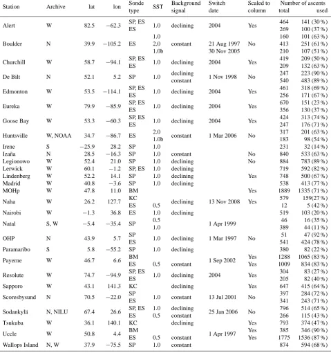
Table 1. Overview of the sonde types used, data processing methods applied for the MOZAIC period (August 1994–March 2009), and soundings available for comparison (see text). Fields are left blank when information is missing or redundant. SST denotes the cathode sensing solution strength of the ECC sondes, whereby SST 1.0 denotes the fully buffered 1.0 % KI solution, SST 0.5 the half-buffered 0.5 % KI, SST 2.0 the unbuffered 2.0 % KI and SST 1.0b the 1.0 % KI, 1/10th buffered solution. MOHp denotes the Meteorological Observatory at Hohenpeißenberg, Germany, OHP the Observatory Haute Provence, France. W denotes the WOUDC archive, N the NDACC archive, and S the SHADOZ archive.

Station Archive lat lon Sonde SST Background Switch Scaled to Number of ascents type signal date column total used

Alert W 82.5 −62.3 SP, ES 1.0 declining 2004 Yes 464 141 (30 %)

ES 269 100 (37 %)

Boulder N 39.9 −105.2 ES

1.0

constant No

160 101 (63 %) 2.0 21 Aug 1997 413 251 (61 %) 1.0b 30 Nov 2005 210 107 (51 %) Churchill W 58.7 −94.1 SP, ES 1.0 declining 2004 Yes 419 209 (50 %)

ES 209 132 (63 %)

De Bilt N 52.1 5.2 SP 1.0 declining 1 Nov 1998 No 247 223 (90 %)

constant 540 483 (89 %)

Edmonton W 53.5 −114.1 SP, ES 1.0 declining 2004 Yes 461 318 (69 %)

ES 256 171 (67 %)

Eureka W 79.9 −85.9 SP, ES 1.0 declining 2004 Yes 670 151 (23 %)

ES 356 130 (37 %)

Goose Bay W 53.3 −60.3 SP, ES 1.0 declining 2004 Yes 424 313 (74 %)

ES 247 176 (71 %)

Huntsville W, NOAA 34.7 −86.7 ES 2.0 constant 1 Mar 2006 No 317 201 (63 %)

1.0b 183 98 (54 %)

Irene S −25.9 28.2 SP 1.0 231 32 (14 %)

Izaña N 28.5 −16.3 SP 1.0 constant No 840 533 (63 %)

Legionowo W 52.4 21.0 SP 1.0 declining No 884 783 (89 %) Lerwick W 60.1 −1.2 SP, ES 1.0 declining 719 592 (82 %) Lindenberg W 52.2 14.1 SP 1.0 declining Yes 748 500 (67 %)

Madrid W 40.8 −3.6 SP 1.0 declining 538 413 (77 %)

MOHp W 47.8 11.0 BM Yes 1889 1335 (71 %)

Naha W 26.2 127.7 KC declining 13 Nov 2008 Yes 579 159(27 %)

ES 0.5 12 5 (42 %)

Nairobi W −1.3 36.8 ES 1.0 declining 519 103 (20 %)

Natal S, W −5.4 −35.4 SP 0.5 1 Apr 1999 46 16 (35 %)

1.0 389 44 (11 %)

OHP N 43.9 5.7 SP 1.0 declining 1 Mar 1997 No 51 47 (92 %)

ES 541 424 (78 %)

Paramaribo S 5.8 −55.2 SP 1.0 declining 380 82 (22 %)

Payerne W 46.7 6.6 BM 1 Sep 2002 Yes 1288 1065 (83 %)

ES 0.5 constant Yes 1009 834 (83 %) Resolute W 74.7 −94.9 SP, ES 1.0 declining 2004 Yes 304 83 (27 %)

ES 205 82 (40 %)

Sapporo W 43.1 141.3 KC declining Yes 647 415 (64 %)

Scoresbysund N 70.5 −22.0 SP 1.0 constant 13 Jul 2001 No 397 284 (72 %)

ES 341 243 (71 %)

Sodankylä N, NILU 67.4 26.6 SP, ES 1.0 declining 25 Jan 2006 No 796 514 (65 %)

ES 0.5 constant 266 115 (43 %)

Tsukuba W 36.1 140.1 KC declining Yes 793 374 (47 %)

Uccle W 50.8 4.4 BM 1 Apr 1997 Yes 385 346 (90 %)

(4)

strengths and buffers (2.0 % KI unbuffered solution, Johnson et al., 2002) and recently with a 1.0 % KI 1/10th buffered so-lution. However, the solutions and techniques used by NOAA are unique and changes are carefully monitored to assure continuity of the record. Therefore, the concern is not with NOAA but with those stations that have used one of the stan-dard buffered solutions, 1.0 % or 0.5 %, but not with the right ECC ozonesonde. NOAA also changed instruments and tech-niques at the Pacific tropical stations it operates (Pago Pago, American Samoa; Hilo, Hawaii; Suva, Fiji; San Cristobal, Ecuador). These stations, because they are not near MOZAIC flight routes, are not included in the present paper.

In this study we analyse 11 stations (Alert, Churchill, Edmonton, Eureka, Goose Bay, and Resolute in Canada; Lerwick, UK; Natal, Brazil; Observatory Haute Provence (OHP), France; Scoresbysund, Greenland; and Sodankylä, Finland) that switched from ES to SP (or vice versa) and/or have operated both sonde types with or without changing the solution strength. At Canadian stations both SP and ES-Z sondes were flown before 2004. After 2004 mainly ES son-des were launched but the 1.0 % solution strength was re-tained (see metadata at WOUDC, the World Ozone and Ul-traviolet Radiation Data Centre).

Recently, the ozonesonde data user community has been addressing how to account for changes in radiosonde instru-mentation that have accompanied ozonesonde changes at a number of stations in the past 5 yr or so (Stauffer et al., 2014). The radiosonde changes propagate to each ozone measure-ment, but mostly at pressures<100 hPa; newer radiosondes mostly affect ozone data after 2009. Thus, these influences are neglected here.

The standard operating procedures (SOP) for the BM son-des are defined by Claude et al. (1987) and have been fol-lowed by MOHp and Payerne. Payerne has higher correction or scaling factors (CF) than MOHp, probably because the pump temperature was assumed constant at 280 K instead of 300 K (see also Jeannet et al., 2007). The CF is determined as the ratio between the total O3 column measured by the

ozonesonde and a nearby independent column measurement, such as from Dobson or Brewer spectrometers. Uccle data, as used here, are normalised following De Backer (1999) rather than utilising the SOPs.

The background current is a major error source for ozonesonde measurements in the upper troposphere, where ozone concentrations are small. The SOP for the BM son-des does not call for correction of the background current. For ECC sondes the conventional correction is to assume that the background current is proportional to the oxygen partial pressure and thus declines with altitude (Komhyr, 1986). This, however, is neither supported by lab studies (e.g. Thornton and Niazy, 1982), nor by the the study of Reid et al. (1996), who found a 7–8 % better agreement be-tween ECC ozonesondes and an UV photometer for tropo-spheric O3concentrations when a constant background

cur-rent was assumed. The recent assessment of ECC SOPs calls

for a constant background current (Smit et al., 2011). The background current (ib) is measured three times during the prelaunch procedure: once the sondes are exposed to puri-fied (ozone-free) air (ib1), once after exposure to O3 (ib2),

and just prior to flight (ib3). We contacted the principle

in-vestigators (PI) in case the treatment of the background cur-rent could not be extracted from the diffecur-rent archives. Only De Bilt (the Netherlands), Huntsville, Legionowo (Poland), Madrid (Spain), OHP, Payerne, Sodankylä, and Uccle re-port their background current values without large data gaps for 1994–2009 (i.e. a few months per year or maximally one whole year is missing). Scoresbysund and Canadian sta-tions have reported background currents to the archives since 2000. Due to the limitations of the Lagrangian match tech-nique presented here (cf. Sects. 2.3 and 3), the influence of the background current on the sonde performance can be thoroughly investigated only at De Bilt, Legionowo, Payerne and Uccle. The latter three, however, report no change in treatment nor large variations of the background current in the 1994–2009 period.

Ozonesonde data can be downloaded from several archives: ftp servers at the WOUDC (World Ozone and Ul-traviolet Radiation Data Centre), NDACC (Network for the Detection of Atmospheric Composition Change), SHADOZ (Southern Hemisphere ADditional OZonesondes), NILU (Norwegian Institute for Air Research), and NOAA (Na-tional Oceanic and Atmospheric Administration). Records from most stations can be found either on the WOUDC or NDACC homepages, or on both. Most tropical stations are now part of the SHADOZ network (Thompson et al., 2003a, b). NILU offers campaign data, for example, measurements from the VINTERSOL campaign (European field campaign studying stratospheric ozone), and high latitude station data. The Intensive Ozonesonde Network Study (IONS) experi-ments (Tarasick et al., 2010; Thompson et al., 2011) over North America have operated in 2004, 2006, 2008, and 2013. This has augmented regular US launches at Boulder (Col-orado), Huntsville (Alabama), and Wallops Island (Virginia) as well as most of the Canadian stations listed in Table 1. The data are archived at NASA/Langley and WOUDC.

(5)

Fig. 1. Distribution of the ozonesonde stations considered in this work (black squares) and to-tal number of measurements from the MOZAIC aircraft program (1994-2009), averaged over a 3◦_×₃◦_latitude_×_{longitude grid. The colour bar indicates the total number of 1-minute averaged MOZAIC}

measurements. MOHp denotes the Meteorological Observatory at Hohenpeißenberg, Germany; OHP the Observatory Haute Provence, France.

37

Fig. 1. Distribution of the ozonesonde stations considered in this work (black squares) and total number of measurements from the MOZAIC aircraft program (1994–2009), summed up over a 3◦×3◦latitude×longitude grid. The colour bar indicates the total number of 1 min averaged MOZAIC measurements. MOHp denotes the Meteorological Observatory at Hohenpeißenberg, Germany; OHP the Observatory Haute Provence, France.

2007 onwards were obtained in February 2011. Huntsville data for 2008 and 2009 were obtained from a NOAA ftp-server in February 2011. Irene (So. Africa), Natal (Brazil) and Paramaribo (Suriname) data were obtained from the SHADOZ database in April 2010, with the exception of data from the Natal site for 1997, which was obtained from the WOUDC. Wallops Island data for 1994, 1995, 2008, and 2009 were obtained from the WOUDC in March and April 2010, while all remaining data were obtained from the NDACC website in April 2010.

MOHp, Payerne, and Uccle typically launch two to three ozonesondes per week, whereas most other sites typically launch one sonde per week. It is important to note that not all sites flew ozonesondes for the entire MOZAIC period, with some stations starting later, particularly tropical ones. Conse-quently, the total number of launches for the entire MOZAIC period (August 1994–March 2009) is quite different from station to station, ranging from 300–400 (e.g. Paramaribo, Irene) to more than 2000 launches (e.g. MOHp, Payerne, Uc-cle, cf. Table 1).

2.2 MOZAIC ozone observations

The MOZAIC program and data from it are described and analysed in detail by Thouret et al. (1998). Here, only the main characteristics are summarised. Dual-beam UV absorp-tion models from Thermo Environment were installed on several commercial aircraft participating in the MOZAIC project. These UV photometers have a response time of 4 s, a detection limit of 2 ppbv, and an uncertainty of±[2 ppbv+

2 %]. For example, for O3=100 ppbv this results in an

un-certainty of±4 ppbv. The quality assurance and control pro-cedures have not changed since the project started in 1994. MOZAIC analysers are inspected annually and periodically calibrated (about every 12 months) with a reference analyser at the French National Institute of Standards and Technology. Additionally, the analysers are checked in-flight with a built-in ozone generator to detect any drift built-in built-instrument efficiency. MOZAIC is considered as a standard reference (for example in Thouret et al., 1998, 2009; Schnadt Poberaj et al., 2009) due to its regular inspections and checks as well as the un-changed quality assurance procedures. However, the recent analyses of both Logan et al. (2012) and Staufer et al. (2013) cast some doubts on the long-term stability of the MOZAIC ozone data.

MOZAIC’s main flight route is the North Atlantic flight corridor, but aircraft also fly to airports in South America, East Asia, and Southern Africa. The flight distribution of the aircraft is shown in Fig. 1. The sounding sites investigated in this work are chosen according to these flight routes. In total, 31 494 flights were available when we downloaded the data (March 2010), covering the period from August 1994 to March 2009. We use 1 min averaged MOZAIC data, which correspond to a horizontal resolution of 10 to 15 km at cruise altitude.

2.3 Comparison methodology

(6)

trajectories to ensure both instrument platforms observe the same air mass. In a companion paper (Staufer et al., 2013), we test and apply this method of comparisons between craft measurements from both MOZAIC and NOXAR air-craft and ozonesonde data from Payerne, Switzerland. Here, we summarise just the main points of this method, which is similar to the trajectory match technique used by Rex et al. (1998) or the trajectory hunting technique described by Danilin et al. (2002). After reconstructing the sonde’s flight path using wind data (speed and direction) from the radiosonde, the trajectory tool LAGRANTO (Wernli and Davies, 1997) is used to calculate 6 day forward and back-ward trajectories for each sounding. Fully three-dimensional trajectories are used because it has been shown, for exam-ple by Stohl and Seibert (1998), that they are more accurate than kinematic isentropic or isobaric trajectories in the tro-posphere. In the stratosphere, isentropic trajectories are of similar accuracy to fully three-dimensional trajectories.

LAGRANTO is forced with six-hourly wind fields from ECMWF’s (European Centre for Medium-Range Weather Forecasts) ERA-Interim reanalysis (1◦horizontal resolution, 61 vertical levels). Trajectories ascending or descending by more than 450 hPa during the six days simulated are ex-cluded to avoid air masses that transport polluted boundary layer air or air from deep stratospheric intrusions. For each trajectory all MOZAIC measurements matching the trajec-tory withinr≤75 km and 12≤0.6 K are collected, then a weighted mean of the aircraft observations is calculated and compared to the ozonesonde measurements at initialisation of the trajectories. For the weighting a time lag compared to the soundings is used to account for the reduced accuracy of trajectories further away in time.

To assess the uncertainty of this technique, Staufer et al. (2013) checked the method for comparison of one instru-ment type with itself, i.e. MOZAIC–MOZAIC self-matches. Assuming that MOZAIC is noise-free, they found mean dif-ferences of±2 %. However, it is important to note that this uncertainty was derived under most favourable conditions, namely a large number of matches and most matches found within the first 50 h of the trajectories. The uncertainty is ex-pected to increase when most matches are found after 50 h since trajectory errors typically accumulate with time. Thus, the temporal distribution of the matches is a limiting factor for this comparison. This issue is discussed in more detail in the beginning of Sect. 3.

As shown by Staufer et al. (2013), the combination of for-ward and backfor-ward trajectories can be used to account for the potential effects of chemistry and mixing along the trajectory paths. These effects are typically more pronounced in the up-per troposphere (UT) than in the lower stratosphere (LS). At Payerne, sonde biases of up to 10 % between forward-only and backward-only trajectories were found. Staufer et al. (2013) further showed that tropospheric photochemistry can-not alone account for the observed differences between for-ward and backfor-ward trajectories. Other factors such as the

different temporal match distribution between the unidirec-tional trajectories or an inaccurate quantification of the mete-orological conditions additionally contribute to the observed differences. For the data considered, very few trajectories were matched in both directions and Staufer et al. (2013) needed to analyse forward and backward trajectories sepa-rately. They showed that by surrounding each trajectory with four additional trajectories, each displaced by 0.5◦latitude and longitude from the central trajectory, the biases could be reduced by half. Furthermore, the sonde bias at Payerne was found to be largely insensitive to the trajectory duration (one or six days). Due to this robustness, and because some sites do not allow reconstructing the balloon flight path since no wind direction or speed data are available, we use all trajec-tories (the central plus the displaced trajectrajec-tories), referred to as the combined trajectory set, unless otherwise mentioned.

For tropical stations (φ <30◦_{N), trajectories were} deter-mined every 1 K in potential temperature at altitudes between 5–15 km. This is in contrast to the mid- and high latitude sta-tions, where similar to Staufer et al. (2013), the trajectories originate every 5 hPa within the UTLS, which is defined as

±125 hPa around the local (lapse-rate defined) tropopause. Without this adaptation, no matches with MOZAIC would have been obtained because the tropical tropopause is much higher than the typical MOZAIC cruise altitude (8–12 km).

3 Ozonesonde comparisons with MOZAIC

Results are first presented as averages over the en-tire MOZAIC period; thereafter the differences between sonde and MOZAIC,1O3=2(sonde−MOZAIC)/(sonde+

MOZAIC), are analysed in more detail by separately dis-cussing the behaviour and changes of1O3 in both the UT

and LS. We first focus on the mid-latitudes (30◦N≤φ≤

60◦N) where most stations are located, then show results for stations at high northern latitudes (φ >60◦N) and for tropi-cal and southern latitudes (φ <30◦N).

Results of the comparisons are limited by the number of matches, which in turn depends on the number of ascents, the location of the station, and the MOZAIC flight paths (see Fig. 1, and Tables 1 and 2). The number of matches per launch site varies considerably. Table 1 shows, for ex-ample, that for the Swiss station Payerne, 1899 ascents can be compared to MOZAIC, while for Natal, which is located in Brazil, only 60 ozonesondes are available for comparison. Thus, stations like Payerne can be analysed in much more detail than stations like Natal.

(7)

Fig. 2. Temporal distribution of the number of matches at different stations. The time lag is positive for

forward-only trajectories and negative for backward-only trajectories. Matches in the stratosphere are

shown in black, while matches in troposphere are shown in gray. The bin size is 10 h.

38

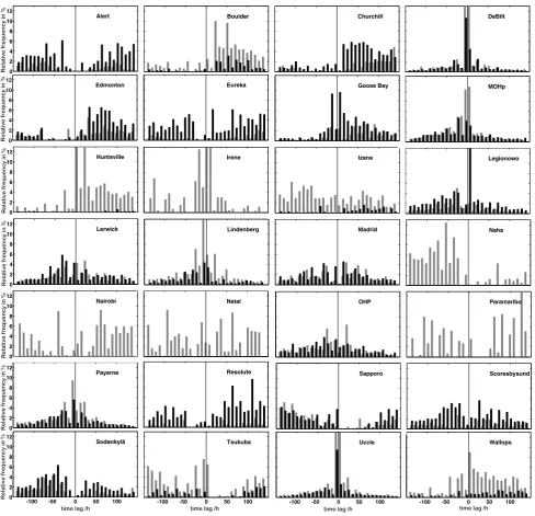
Fig. 2. Temporal distribution of the number of matches at different stations. The time lag is positive for forward-only trajectories and negative for backward-only trajectories. Matches in the stratosphere are shown in black, while matches in troposphere are shown in gray. The bin size is 10 h.

southern latitudes, or in Japan, have most matches after 50 h. Staufer et al. (2013) tried to systematically assess the un-certainty for different time lags but the uneven distribution of the MOZAIC self-matches, i.e. hardly any matches af-ter 50 h, prevented them from doing so. However, by ex-cluding matches from the first 24 h, uncertainty increased by 1–2 %, particularly in the UT, indicating an increas-ing uncertainty with increasincreas-ing trajectory duration (Staufer et al., 2013). Thus, stations that are either closer to highly

frequented MOZAIC airports or whose balloon trajectories cross the main MOZAIC flight path over the North Atlantic are favoured by this Lagrangian approach. These favoured stations are mainly located in Europe. For stations outside of Europe, larger errors bars in1O3certainly reflect the

(8)

3.1 Results for mid-latitude stations

3.1.1 MOHp/Payerne/Uccle

During the MOZAIC period (1994–2009) only three stations flew BM ozonesondes. Uccle and Payerne switched to ECC sondes (ES-Z type operated with 0.5 % KI half buffered sens-ing solution) in April 1997 and September 2002, respec-tively; Hohenpeißenberg (MOHp) still launches BM son-des, and thus is the only remaining BM station worldwide. Sample sizes from these three stations are largest because 2–3 sondes are flown per week at each of these sites, and the stations are located close to the main MOZAIC airports and flight routes. The percentage of matched ozonesondes is largest at Uccle (≈90 %) and smallest at MOHp (71 %). This disparity is related partly to the location of Uccle, which lies close to Brussels airport and the main flight route of aircraft over northern and western Europe (see Fig. 1). In addition, MOHp data from the WOUDC are reported on fewer pres-sure levels than at Payerne and Uccle.

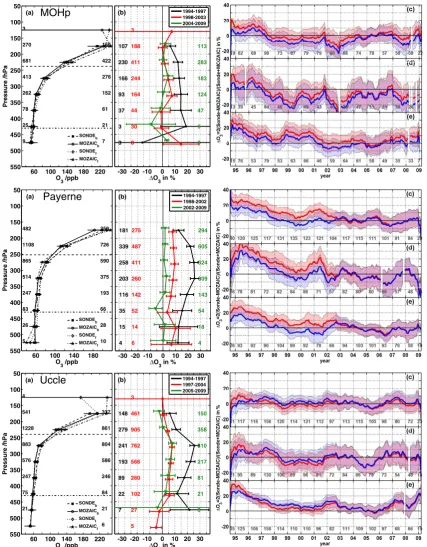
The 16 yr mean O3 concentrations from sondes and

MOZAIC are shown in Fig. 3a. They show a striking agree-ment. The height of the lapse-rate defined tropopause is de-rived only from the sondes used in this comparison, resulting in a mean tropopause pressure of 250 hPa. Sonde–MOZAIC differences obtained from the unidirectional trajectories are negligibly small at all altitudes for both MOHP and Uccle, but range up to 5 % at Payerne (see also Staufer et al., 2013), although the differences in absolute concentrations are on the order of a few ppb in the troposphere. For all stations, the O3

concentrations obtained from forward-only trajectories are systematically higher than from backward-only trajectories.

Figure 3b shows the mean relative differences between sonde and MOZAIC split into three different periods. The first period, 1994–1997, is characterised by large differences between BM sondes and early MOZAIC observations. At MOHp the sondes exceed MOZAIC by 10–15 %, while at Payerne and Uccle even higher offsets are found (up to 25 % in the vicinity of the tropopause). Mean 1994–1997 differ-ences are lowest (5 % at MOHp and 10 % at Payerne, Uccle) at the 175 hPa level, where mean O3concentrations are on

the order of 200 ppb. After 1997/1998 the mean differences drop to less than 10 % at all three stations, at all altitudes.

Figure 3c–e show the time series of 13 month moving average monthly mean differences. The lower stratosphere (Fig. 3c) includes only trajectories where the difference in pressure between the trajectory at initialisation (p(t=0)) and the tropopause pressure (pTP) is smaller than 15 hPa.

Figure 3d contains a narrow tropopause band with |p(t=

0)−pTP|<15 hPa. The values chosen are similar to those

of Thouret et al. (2006), who also considered a 30 hPa thick tropopause zone. The time series of the tropopause dif-ferences is more uncertain and more variable because the strongest O3gradients are typically found in the vicinity of

the tropopause. Figure 3e comprises the upper troposphere

and includes all trajectories satisfying p(t=0)−pTP≥

15 hPa. All calculations follow the methodology laid out in Staufer et al. (2013); however, 50 hPa pressure intervals are used here instead of 1 km altitude bins.

At MOHp, the CF corrects for the low BM sonde bias in the LS, except for the 1994–1997 period when the applica-tion of the CF results in a high bias compared to MOZAIC. For the UT, application of the CF is counterproductive for al-most all periods. In contrast, at Payerne the agreement with MOZAIC in both the UT and LS is better when no scaling is applied. Whereas Stübi et al. (2008) recommended scaling both sonde types to column O3, Staufer et al. (2013)

sug-gest that the transition from BM to ECC sondes is smoother when the BM sondes remain unscaled, at least for the LS as defined here. The homogenised Uccle and MOZAIC data show differences of less than 5 % in the LS (Fig. 3c), but the homogenisation does not remove the high offset in the mid-1990s in the troposphere (Fig. 3e). However, their CF, whose calculation differs from the usual approach, reduces the bias compared with MOZAIC to 5 % in the UT after 1996. Our analysis qualitatively confirms results from Schnadt Poberaj et al. (2009) for the European ozonesonde stations. Further-more, our analysis shows that the mean discrepancies at Uc-cle from 1994–2001 can be traced back to the use of BM sondes. Our results for the free troposphere (p >430 hPa) also qualitatively agree with the recent study of Logan et al. (2012), who found that the tropospheric portion of BM sonde data before 1998 should be discarded for trend analysis due to the mismatch with MOZAIC and long-term ozone mea-surements from alpine sites. The anomalous peak in the Uc-cle tropospheric data in 2007 is present in our analysis, al-though in 2002 a peak of similar magnitude is also found. However, note that the peak in 2002 is not present in the UT, when trajectories satisfyingp(t=0)−pTP≥30 hPa are used

instead (not shown). The high bias in UT O3 compared to

MOZAIC observed at all three BM sonde sites for the 1994– 1997 period remains unexplained.

3.1.2 De Bilt

In contrast to Payerne and Uccle, at De Bilt SP sondes oper-ated with a 1.0 % KI cathode electrolyte have been used dur-ing the entire MOZAIC period. A smaller number of ozone soundings is available from this launch site compared to MOHp, Payerne, and Uccle because typically just one sound-ing is launched per week. Despite this, 90 % of the soundsound-ings could be matched with MOZAIC (Table 1).

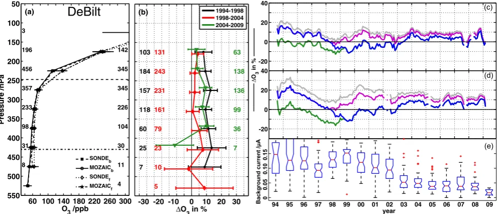
Similar to MOHP, Payerne, and Uccle, the 16 yr mean O3 concentrations from both De Bilt and MOZAIC agree

to within 10 % at all altitudes (Fig. 4a). However, the dif-ference between ozonesondes and MOZAIC shows a distinct time dependence,1O3amounts to 15 % in the LS and 20 %

(9)

39

Fig. 3. Comparison between MOZAIC O3measurements and ozonesondes from MOHp, Payerne, and Uccle. (a) 16 yr average O3profiles

from sonde and MOZAIC binned into 50 hPa layers. Numbers on the left and right denote the number of soundings using 6 day backward-only and forward-only trajectories, respectively. The dashed horizontal line denotes the tropopause, the dash-dotted horizontal line the level up to which Logan et al. (2012) compared ozonesondes with MOZAIC. (b) Relative differences1O3=2(sonde−MOZAIC)/(sonde+MOZAIC)

split into three periods. The number of sondes available for comparison is displayed for each period on the sides. Time series of1O3with

(10)

Fig. 4. Comparisons of De Bilt ozonesondes with MOZAIC measurements. (a) and (b): As for Fig. 3a–b. (c) and (d): time series of1O3

for the LS (c) and UT (d), respectively. Time series are shown for the difference resulting from using the operating procedures described in Table 1 (blue line), with no correction for background signal (gray line), with a constant background current correction (green line), and with the application of an altitude-dependent background correction (purple line). (e): annual statistical distribution of the background current used to process the ozonesonde data. The median is depicted as a horizontal solid red line, the 90 % confidence interval as the notches. The box limits correspond to the 75 % and 25 % quartiles. The whiskers extend out to the maximum or minimum values, or to 1.5 times either the 75 % or 25 % quartile if there are data beyond this range. Outliers are identified with red crosses.

background signal, the main source of uncertainty in calcu-lating tropospheric O3partial pressures, which shows a

sig-nificant trend over this period (Fig. 4e). Prior to 2003 the background current was high (0.10–0.16 µA) and highly vari-able. The reduced background current after 2003 is a conse-quence of a change in prelaunch procedure. Chemicals are renewed more often and the signal is measured outdoors just prior to launch instead of being measured indoors (A. Piters, personal communication, 2012). With typical values of<0.06 µA, the background current at De Bilt now agrees well with the signals measured at Payerne and Uccle (0.03– 0.04 µA). The drop of1O3 to below 0 % from 1998–2002

can be explained by two factors, the large background current values and the change in background current treatment. Since November 1998 a constant background current has been used to process the data instead of a background current that de-clines with altitude. In the case of having large background current values, when a constant value is subtracted from the measured cell current much lower O3 partial pressures are

obtained than when an altitude-dependent background cur-rent is subtracted. This feature is more pronounced in the up-per troposphere than in the lower stratosphere since smaller O3partial pressures are measured. The hypothesis that the

background current values and the changing background cur-rent treatment are responsible for the low O3 partial

pres-sures measured by sondes is further supported by the fact that the differences between sonde and MOZAIC are more

stable (i.e.1O3do not drop to below 0 %) before 2003 if the

data are processed with an altitude-dependent background current, especially in the LS (Fig. 4c). After 2003, when the mean background values drop below 0.06 µA, the spread in the results resulting from different correction schemes (alti-tude dependent or constant) is significantly smaller. During this period, the agreement with MOZAIC in the LS is better than 5 % when a constant background is subtracted, and bet-ter than 10 % when an altitude-declining background current is subtracted. In the UT, the agreement is better than 10 % with a constant background current and better than 15 % with an altitude-declining background current.

3.1.3 Legionowo

(11)

Fig. 5. Comparison of ozonesondes with MOZAIC measurements. As for Fig. 3, but for Legionowo.

42

Fig. 5. Comparison of ozonesondes with MOZAIC measurements. As for Fig. 3, but for Legionowo.

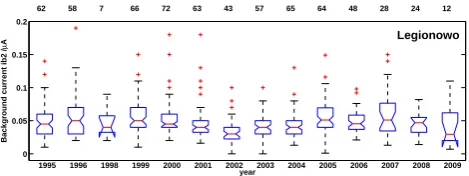
0 0.05 0.1 0.15 0.2

year

Background current ib2 /

µ

A

62 58 7 66 72 63 43 57 65 64 48 28 24 12

1995 1996 1998 1999 2000 2001 2002 2003 2004 2005 2006 2007 2008 2009

Legionowo

Fig. 6. Annual statistical distribution of the background currentib2used to process Legionowo ozonesonde data. Note thatib2is not reported to the archives for every launch and data prior to 26 Jan-uary 1995 were not reported to the WOUDC archive.

43

Fig. 6. Annual statistical distribution of the background currentib2

used to process Legionowo ozonesonde data. Note thatib2is not

reported to the archives for every launch and data prior to 26 Jan-uary 1995 were not reported to the WOUDC archive.

Uccle, MOHp, and De Bilt. In the LS, differences between sonde and MOZAIC are large from 1994–1997 (15–20 %), then decrease to below 10 % from 1998–2001, and remain around 10 % thereafter. The LS time series of the1O3at both

Legionowo and De Bilt show similar patterns if both data are processed assuming an altitude-declining background signal. The five European stations analysed above reveal pro-nounced similarities in the sonde–MOZAIC differences. All show large discrepancies of 20–25 % in the mid-nineties (1994–1997), followed by smaller differences of 5–10 % in the subsequent years. MOZAIC’s UV photometers are regu-larly checked for significant variations and recalibrated each year but it is remarkable that both sonde types (BM and ECC) reveal temporal similarities in1O3. It is not straightforward

to understand this behaviour, but it appears premature to at-tribute these discrepancies only to errors derived from the ozonesonde observations. Although it cannot be ruled out completely that the Lagrangian technique may have system-atic problems, a slight error in the long-term stability of

MOZAIC in the mid-nineties needs to considered. This has also been discussed by Logan et al. (2012), who found an increase in the MOZAIC bias from 1994–2009 over Frank-furt/Munich compared with the alpine surface site Zugspitze (Germany).

As already mentioned, the number of matches and the cor-responding temporal distribution affect the application of the match approach. The ozonesonde stations presented above are clearly favoured by their location, the large number of ascents and matches (cf. Table 2), and the temporal distribu-tion of their matches, which are mostly found within the first 50 h (cf. Fig. 2). These conditions, however, do not apply to the other stations presented below. Consequently, less pre-cise deductions about1O3and the influence of instrument

variations on the sonde performance can be made.

3.1.4 Lindenberg/Madrid/OHP

(12)

Fig. 7. Comparison of ozonesondes with MOZAIC measurements. As for Fig. 3, but for Lindenberg,

Madrid, and the Observatory Haute Provence (OHP). ES sondes are flown at OHP since March 1997,

while SP sondes were used before. Both are operated with a 1.0% electrolyte.

Fig. 7. Comparison of ozonesondes with MOZAIC measurements. As for Fig. 3, but for Lindenberg, Madrid, and the Observatory Haute Provence (OHP). ES sondes have been flown at OHP since March 1997, where SP sondes were used before. Both are operated with a 1.0 % electrolyte.

(13)

Table 2. Total number of matches, matched trajectories and ascents used for the different launch sites included in this study.

Station

Total number of

matches matched matched sonde trajectories ascents

Alert 2703 1051 241

Boulder 5986 1816 459

Churchill 5271 1994 341

De Bilt 41 520 13 277 706

Edmonton 9301 3269 489

Eureka 2935 1077 281

Goose Bay 10 942 3979 489

Huntsville 5250 1543 299

Irene 743 219 32

Izaña 7450 2261 533

Legionowo 22 384 8118 783

Lerwick 16 048 5958 592

Lindenberg 5718 2080 500

Madrid 10 204 3381 413

MOHp 17 576 5885 1335

Naha 2589 693 164

Nairobi 1783 397 103

Natal 739 142 60

OHP 11 060 3702 471

Paramaribo 792 204 82

Payerne 70 336 21 439 1899

Resolute 1599 627 165

Sapporo 8198 2890 415

Scoresbysund 13 004 4699 572

Sodankylä 9559 3530 629

Tsukuba 3909 1468 374

Uccle 96 746 30 007 1882

Wallops 10 854 3631 594

total 395 203 129 340 14 859

at Lindenberg less than 70 % are matched, partly because fewer trajectories are initialised. Similar to MOHp, the other DWD (German Weather Service) station, data from Linden-berg are reported on fewer pressure levels than at Madrid, OHP, and all other sites. The tropopause height at Linden-berg calculated using the soundings available for comparison is 20–30 hPa higher than several European stations, including Madrid, OHP, and Legionowo (Fig. 7a).

Between 300–400 hPa there are some sonde–MOZAIC differences (up to 10 %) between the backward- and forward-only trajectories, with the backward-forward-only trajectories yield-ing larger sonde biases (Fig. 7a). As mentioned previously, and as described in detail by Staufer et al. (2013), this may result from chemical processing along the trajectories, differ-ent temporal match distributions between the unidirectional trajectories, and inaccurate quantification of the meteorolog-ical conditions in the UT.

The lower stratospheric sonde–MOZAIC differences at Lindenberg, Madrid, and OHP range from−5 % (OHP) to 5– 10 % (Lindenberg, Madrid), while in the troposphere they are somewhat larger (Fig. 7b). Large discrepancies between son-des and MOZAIC are found in the stratosphere at both Lin-denberg and Madrid from 1994–1996 (up to 15 %) (Fig. 7c). In the troposphere the discrepancies increase in the 1990s at Madrid, while at Lindenberg the sonde data are 15–30 % larger than MOZAIC from 1994–1998.

Our analysis indicates that there is no obvious break in the

1O3time series over OHP resulting from the switch of ECC

sonde manufacturer in March 1997. There is, however, a de-crease in tropospheric bias after 1997, although this cannot be attributed to the change in ECC sonde type (and retaining a 1.0 % KI) since several other stations show similar devia-tions during this period as well. The times series in the LS is too noisy to draw any firm conclusions.

3.1.5 Churchill/Edmonton/Goose Bay

The sonde–MOZAIC comparison at the Canadian mid-latitude stations Churchill, Edmonton, and Goose Bay is pre-sented in Fig. 8. Because of the MOZAIC flight distribu-tion, most matches are obtained from forward trajectories (Fig. 8a), with most trajectories originating from the lower stratosphere. In total, 350–500 ozonesondes can be matched with MOZAIC at these stations, the equivalent of only one third the sample size of the European BM stations.

In the lower stratosphere, the1O3time series are

qualita-tively similar, especially for Edmonton and Goose Bay. The sondes overestimate MOZAIC by up to 5 % at Goose Bay, and by up to 15–35 % at Edmonton and Churchill from 1994– 1996, but then underestimate O3compared to MOZAIC from

1997–1999 (Fig. 8c). Thereafter, the sonde–MOZAIC bias becomes positive again, ranging between 5–15 %, depending on the station. The results suggest no statistically significant differences in the mean lower stratospheric deviations (at the 90 % confidence level; see Fig. 8b). Although there are only a few tropospheric matches, the discrepancies at Goose Bay from 1995–1996 (ranging between 15–20 %) are similar to those observed at European stations (Fig. 8e).

3.1.6 Boulder/Huntsville/Wallops Island

Matches for the United States stations are obtained mostly from forward trajectories originating in the upper tropo-sphere, particularly at Huntsville and Wallops Island (see Fig. 9a). Note that as for the Canadian stations, the number of matched ozone soundings is much lower than at MOHp, Payerne, or Uccle. This is likely in part due to the low mea-surement frequency and the position of these stations.

(14)

Fig. 8. Comparisons of ozonesondes with MOZAIC measurements. As for Fig. 3, but for Churchill,

Edmonton, and Goose Bay. At all three launch sites both SP and ES-Z sondes were flown before 2004.

After 2004 mainly ES sondes were launched but the 1.0 % solution strength was retained

Fig. 8. Comparisons of ozonesondes with MOZAIC measurements. As for Fig. 3, but for Churchill, Edmonton, and Goose Bay. At all three launch sites both SP and ES-Z sondes were flown before 2004. After 2004 mainly ES sondes were launched but the 1.0 % solution strength was retained.

(15)

Fig. 9. Comparison of ozonesondes with MOZAIC measurements. As for Fig. 3, but for Boulder,

Huntsville, and Wallops Island. For each period in (b) a different sensing solution was used at

Boul-der and Huntsville.

Fig. 9. Comparison of ozonesondes with MOZAIC measurements. As for Fig. 3, but for Boulder, Huntsville, and Wallops Island. For each period in (b) a different sensing solution was used at Boulder and Huntsville.

(16)

twice, in August 1997 and November 2005 (Table 1). The Boulder sondes exceed MOZAIC observations by<5 % at pressure<300 hPa for most of the time periods considered, but show a positive offset of up to 20 % in the lower strato-sphere from 1995–1996 (Fig. 9c). This provides further ev-idence that MOZAIC perhaps underestimates O3compared

to the sondes from 1994–1997.

Ozone soundings began at Huntsville in 1999. From all observations considered here, only very few backward trajec-tories are matched so the O3time series is almost entirely

de-termined from forward trajectories. Sondes exceed MOZAIC by up to 10 %, depending on altitude (Fig. 9b), with slightly higher values being observed after the change from a 2.0 % KI unbuffered solution to a 1.0 % KI 1/10th buffered solu-tion in March 2006.

Above 350 hPa, ozonesondes flown from Wallops Island show similar results from 1994–2009 with sonde measure-ments exceeding MOZAIC by 5–15 % (Fig. 9b). These val-ues agree well with results from Schnadt Poberaj et al. (2009), who also show a positive sonde bias of 5–20 % com-pared to MOZAIC from 1994–2001. Below 350 hPa the son-des tend to measure more O3from 2005–2009 than in

previ-ous periods, in particular between 350–450 hPa. Such a trend is not visible at other sites.

3.1.7 Sapporo/Tsukuba

The 16 yr mean O3 concentrations obtained from sondes

flown at Tsukuba and Sapporo, and from MOZAIC agree within 5 % in the troposphere (Fig. 10a). However, there are differences in the stratospheric performance (typically at pressures <250 hPa) from forward-only and backward-only trajectories at Tsukuba. The agreement of sondes with MOZAIC also tends to evolve differently at Sapporo and Tsukuba (Fig. 10b). Although both stations used the same sonde type (KC-79 until summer 1997, KC-96 from summer 1997 to December 2009), from 2005–20091O3is positive

(10–20 %) at pressures <350 hPa at Tsukuba but negative (−10 %) at Sapporo.

As already mentioned, the time lag between sonde– MOZAIC matches can be an important factor for the com-parison. The temporal distribution of the individual matches is provided in Fig. 2; however, this distribution might be biased since it does not account for the averaging of the matches along each trajectory – some trajectories contain more individual matches than others – nor for the weighting of matches along the trajectories. It does, though, provide an idea of the mean time lag between MOZAIC measurements and the soundings. In contrast to most of the European sta-tions, the majority of stratospheric matches at non-European stations are not found within the first 50 h of air parcel travel time. Rather, many matches occur at the end of the trajec-tories where they have already travelled more than 100 h. In our companion paper (Staufer et al., 2013), a 2 % uncer-tainty was found when testing this matching technique using

MOZAIC–MOZAIC self-matches. This comparison found that most matches (50 %) occurred within the first two days (48 h) of trajectories. Thus, in the case of the Japanese sta-tions with almost no matches in the first two days of the tra-jectories, this uncertainty is likely to be higher than 2 % due to accumulated trajectory errors and may explain the discrep-ancies observed. The results for Sapporo and Tsukuba are therefore less reliable.

3.2 High latitude stations

3.2.1 Lerwick/Scoresbysund/Sodankylä

Results for the high latitude stations included in this study are presented in Fig. 11. At these sites the tropopause is lo-cated at pressures<300 hPa except for Lerwick, where it is located at pressures<250 hPa. A larger sample is obtained for the LS compared to the UT because the height of the tropopause is lower at high latitudes than at mid-latitudes, while MOZAIC’s cruise altitude remains constant (8–12 km) independent of latitude. For all three high latitude stations the sondes exceed MOZAIC by 5–10 % in the stratosphere and by 10–15 % in the troposphere. For Lerwick and Sodankylä the differences between sondes and MOZAIC obtained from backward-only trajectories are systematically larger than for forward-only trajectories (5 %) (Fig. 11a).

Scoresbysund is among those stations that have used ES ozonesondes without the right standard buffered solution. Extensive laboratory and field work showed that differ-ences of 5–10 % can be observed if the wrong solution is used (e.g. Kivi et al., 2007; Smit et al., 2007; Deshler et al., 2008). At Scoresbysund, after the change from SP to ES sondes in 2001, measured O3 concentrations are

systemati-cally 5 % higher at all altitudes (Fig. 11b). This is in accor-dance with the JOSIE (Smit et al., 2007) and BESOS exper-iments (Deshler et al., 2008), which showed that ES sondes had systematic high bias of around 5 % compared to SP son-des when both were operated with a 1.0 % KI cathode sens-ing solution.

(17)

Fig. 10. Comparisons of ozonesondes and MOZAIC measurements. As for Fig. 3, but for Sapporo and

Tsukuba.

47

Fig. 10. Comparisons of ozonesondes and MOZAIC measurements. As for Fig. 3, but for Sapporo and Tsukuba.

preparations is small, and therefore this change is not likely to influence the sonde performance at Sodankylä.

At Lerwick sondes exceed MOZAIC, in particular in the upper troposphere in the early years (>20 % from 1994– 1996; see Fig. 11c). 1O3 in the LS is <10 % for most

of 1994–2009, similar to most ECC stations. According to the information given at the WOUDC, Lerwick frequently changed between SP and ES sondes, both flown with a 1.0 % KI electrolyte. We contacted the PIs for more information on the exact switch dates of the ECC sensors so as to analyse the data set more thoroughly. However, satisfying answers could not be provided by them. We therefore cannot assess whether and how the frequent changes from SP to ES sondes and vice versa influences the agreement with MOZAIC data.

3.2.2 Alert/Eureka/Resolute

(18)

Fig. 11. Comparisons of ozonesondes and MOZAIC measurements. As for Fig. 3, but for Lerwick,

Scoresbysund, and Sodankyl¨a. Scoresbysund changed from SP to ES sondes in July 2001. The 1.0% KI

was retained. Sodankyl¨a mainly used SP sondes (1.0% KI) before switching to ES sondes (0.5% KI) in

January 2006.

Fig. 11. Comparisons of ozonesondes and MOZAIC measurements. As for Fig. 3, but for Lerwick, Scoresbysund, and Sodankylä. Scoresby-sund changed from SP to ES sondes in July 2001. The 1.0 % KI was retained. Sodankylä mainly used SP sondes (1.0 % KI) before switching to ES sondes (0.5 % KI) in January 2006.

(19)

100 200 300 400 50 100 150 200 250 300 350 400 450 500 550

O₃ /ppb

Alert Pressure /hPa 27 96 35 15 8 5 3 19 81 46 26 10 SONDE b MOZAIC_b SONDE f MOZAIC_f

100 200 300 400 50 100 150 200 250 300 350 400 450 500 550

O₃ /ppb

Eureka Pressure /hPa 26 116 58 19 15 15 19 69 44 14 6 4 SONDE b MOZAIC_b SONDE f MOZAIC_f

100 200 300 400 50 100 150 200 250 300 350 400 450 500 550

O₃ /ppb

Resolute Pressure /hPa 13 92 34 16 10 6 4 35 24 7 4 3 SONDE b MOZAIC_b SONDE f MOZAIC_f

Fig. 12. 16-year average (1994-2009)

O

3

profiles from sondes flown at Alert, Eureka, and Resolute,

and from MOZAIC. Data are grouped into 50 hPa layers. Numbers on the left and right indicate the

number of soundings using 6-day backward-only (subscript b) and forward-only trajectories (subscript

f), respectively.

49

Fig. 12. 16 yr average (1994–2009) O3profiles from sondes flown at Alert, Eureka, and Resolute compared to O3profiles from MOZAIC.

Data are grouped into 50 hPa layers. Numbers on the left and right indicate the number of soundings using 6 day backward-only (subscript b) and forward-only trajectories (subscript f), respectively.

3.3 Tropical stations

3.3.1 Izaña

Results for the troposphere using only forward trajectories reveal a sonde–MOZAIC bias similar to that observed at Eu-ropean sites such as Legionowo or Madrid. In contrast, re-sults using only backward trajectories reveal a large offset between sondes and MOZAIC (>20 %, see Fig. 13a). The geographical distribution of matches (Fig. 14) shows two ma-jor peaks in the backward direction, one over the Canary Is-lands and one over the east coast of the United States, while most matches in the forward direction are found over the Mediterranean Sea, with no pronounced peaks. The spatial distribution is also reflected in the temporal distribution of matches, since no pronounced peaks are observed (Fig. 2). Most matches with MOZAIC observations therefore occur after 3 days travel along the trajectory paths, where the tra-jectories are expected to be less accurate. It may also be pos-sible that O3production takes place over the course of the

12 day trajectories given that the photochemical lifetime of tropospheric O3is expected to be shorter in the subtropics

and tropics than in the mid- and high latitudes (e.g. Logan et al., 1981).

Differences between the two data sets are less than 5 % in the stratosphere, and no trend in performance is found (Fig. 13b). It appears that Fig. 13c does not support this statement, but it can be explained by the different calcula-tion of1O3. The calculation of1O3 in Fig. 13b is based

on monthly mean differences. Some months contain more ascents than others. Ascents in months with few matches are therefore weighted stronger than ascents in months with many matches, which is not the case for the calculation used in Fig. 13b, where all matched sonde ascents contribute with

the same weight to1O3. No statistically significant changes

in bias are found in the troposphere either, but again note that the the sonde data have a greater positive bias from 1994–1995 compared to the subsequent four to five years (Fig. 13e).

3.3.2 Nairobi/Irene/Naha/Paramaribo/Natal

As a result of the distribution of MOZAIC flights, only very few matches with ozonesondes in the tropics and Southern Hemisphere were found (less than one third of all sondes flown). Furthermore, comparison was only possible in the troposphere because the aircraft cruise altitude is usually be-low the height of the tropopause. Because of the very small sample size, only the 16 yr (1994–2009) average results are provided (see Fig. 15). In addition, the rather poor tempo-ral distribution of matches adds to the uncertainty (Fig. 2). Most stations agree with MOZAIC to within 10 % at pres-sures>400 hPa and within 20 % (10–20 ppbv) at pressures

(20)

Fig. 13. Comparison of ozonesonde and MOZAIC ozone measurements. As for Fig. 3, but for Iza˜na. SP

sondes operated with 1.0% electrolyte are used for the entire period.

50

Fig. 13. Comparison of ozonesonde and MOZAIC ozone measurements. As for Fig. 3, but for Izaña. SP sondes operated with 1.0 % elec-trolyte are used for the entire period.

Fig. 14. Spatial distribution of matches between MOZAIC aircraft observations and (a) backward

trajec-tories or (b) forward trajectrajec-tories initialised at Iza˜na at altitudes between 5-15km. The colour bar shows the total number of matches, averaged over a3◦_×₃◦_grid

51

Fig. 14. Spatial distribution of matches between MOZAIC aircraft observations and (a) backward trajectories or (b) forward trajecto-ries initialised at Izaña at altitudes between 5–15 km. The colour bar shows the total number of matches, summed up over a 3◦×3◦grid.

in April 2010) evidently reflect high Paramaribo ozone archives.

4 Summary and conclusions

Because of the annual inspection and calibration of the highly accurate (±2 % uncertainty) UV-photometers, the MOZAIC data are often considered as the standard data set to validate other ozone data sets (e.g. Thouret et al., 1998; Schnadt Poberaj et al., 2009) or chemistry-transport mod-els (e.g. Law et al., 2000; Brunner et al., 2003; Teyessè-dre et al., 2007). However, recent analyses cast some doubt on the long-term stability of the MOZAIC data; partic-ularly the differences between MOZAIC and NOXAR in 1995–1997 (Staufer et al., 2013) and the increase in bias

between Frankfurt/Munich MOZAIC and the alpine surface site Zugspitze from 1994–2009 (Logan et al., 2012) raised some concern. One of the main purposes of this paper was to investigate the long-term stability and consistency of both MOZAIC and ozonesonde data. To do so, 16 yr (1994–2009) of O3observations from MOZAIC aircraft were compared

with measurements from balloon-borne ozonesondes using 6 day, three-dimensional trajectories. Match criteria of 75 km maximum horizontal distance and 0.6 K maximum poten-tial temperature difference (≈ ±20 m) were chosen to ensure that measurements from both platforms sampled the same air mass. This method relies on 14 859 balloon ascents that are matched with observations from MOZAIC flights, yield-ing a total of 129 340 independent match trajectories. O3

measurements from soundings and airliners are averaged in 50 hPa segments to examine tropical to high latitude data.

The present analysis confirms that, at least during the MOZAIC period, ozonesondes provide a reliable tool for investigating atmospheric O3 climatologies, even in

prox-imity of the tropopause, where O3 partial pressures are

low and measurement uncertainty high. The differences be-tween ozonesondes and MOZAIC are typically smaller in the lower stratosphere (5–10 %) than in the upper troposphere (10–15 %), where the uncertainty of ozonesondes is higher. Stratospheric O3climatologies from ozonesondes also agree

within 5–10 % with satellites such as MLS (Microwave Limb Sounder, e.g. Jiang et al., 2007) and OMI (Ozone Monitoring Instrument, e.g. Thompson et al., 2012).

(21)

25 50 75 100 125 50 100 150 200 250 300 350 400 450 500 550

O₃ /ppb

Irene Pressure /hPa 3 3 4 5 7 5 8 3 5 5 6 5 5 SONDE_b MOZAIC b SONDE_f MOZAIC f

25 50 75 100 125 50 100 150 200 250 300 350 400 450 500 550

O₃ /ppb

Naha Pressure /hPa 6 7 7 8 14 11 11 8 3 26 33 39 44 30 30 18 8 SONDE_b MOZAIC b SONDE_f MOZAIC f

25 50 75 100 125 50 100 150 200 250 300 350 400 450 500 550

O₃ /ppb

Nairobi Pressure /hPa 4 14 15 19 22 12 19 17 11 9 11 7 10 11 8 SONDE_b MOZAIC b SONDE_f MOZAIC f

25 50 75 100 125 50 100 150 200 250 300 350 400 450 500 550

O₃ /ppb

Natal Pressure /hPa 3 11 11 9 3 3 3 9 10 6 7 SONDE_b MOZAIC b SONDE_f MOZAIC f

Fig. 15. Comparison of MOZAIC ozone measurements at tropical and southern latitude ozonesonde

stations. As for Fig. 12, but for Irene, Naha, Nairobi, Natal, and Paramaribo.

52

Fig. 15. Comparison of MOZAIC ozone measurements at tropical and southern latitude ozonesonde stations. As for Fig. 12, but for Irene, Naha, Nairobi, Natal, and Paramaribo.

et al., 2007; Deshler et al., 2008, where ozonesondes were also compared to the UV-photometer technique). However, before 1998 discrepancies of up 25 % are observed and one therefore could argue that the ozonesondes should only be trusted after 1998 since the UV photometry technology used by the MOZAIC program is expected to be more precise, particularly at the low ozone concentrations typical of the UTLS. The MOZAIC instruments are also inspected annu-ally and regularly calibrated, which is not the case for single-use balloon-borne ozonesondes. The fact, however, that 10 of the 20 time series shown in Fig. 16 indicate large pos-itive differences compared to MOZAIC in the mid-1990s, followed by a systematic tendency to smaller differences in subsequent years, casts some doubt on the explanation that the differences are due solely to errors stemming from the ozonesondes. It is remarkable that various sonde types re-veal similar behaviour, namely BM (Brewer-Mast) and ECC (electrochemical cells manufactured by either SP or ES). In

view of the fact that three different manufacturers were in-volved in building these instruments, it is not straightforward to understand this behaviour. Likewise, however, MOZAIC operated five aircraft instruments simultaneously, and it is also not clear how these instruments could explain the ob-served differences, even though they are identically con-structed, maintained, and calibrated. A comparison between Payerne BM sondes and O3measurements made during the

NOXAR B747 project from 1995–1996 showed a smaller offset of around 15 % (scaled) compared to MOZAIC, which may indicate a small drift in the MOZAIC calibration (see Staufer et al., 2013).

(22)

53

Fig. 16. Time series of the relative differences between ozonesondes and MOZAIC measurements (1O3in %) in the upper troposphere.

These time series comprise 20 of the 28 launch sites considered in this work (the 8 remaining have too few matches with MOZAIC to be included here). Note the large differences at nearly all sites from 1994 to 1998, and the systematic tendency for smaller differences at 10 of these stations thereafter, three using BM sondes (MOHp, Payerne, Uccle) and seven using SP or ES ECC sondes (De Bilt (SP), Legionowo (SP), Lindenberg (SP), Goose Bay (SP, ES), Edmonton (SP, ES), Lerwick (SP, ES), and Izaña(SP)). Bold lines:1O3time series with CF