Clim. Past, 9, 393–421, 2013 www.clim-past.net/9/393/2013/ doi:10.5194/cp-9-393-2013
© Author(s) 2013. CC Attribution 3.0 License.
EGU Journal Logos (RGB)
Advances in
Geosciences
Open Access
Natural Hazards
and Earth System
Sciences
Open Access
Annales
Geophysicae
Open Access
Nonlinear Processes
in Geophysics
Open Access
Atmospheric
Chemistry
and Physics
Open Access
Atmospheric
Chemistry
and Physics
Open Access
Discussions
Atmospheric
Measurement
Techniques
Open Access
Atmospheric
Measurement
Techniques
Open Access
Discussions
Biogeosciences
Open Access Open Access
Biogeosciences
DiscussionsClimate
of the Past
Open Access Open Access
Climate
of the Past
Discussions
Earth System
Dynamics
Open Access Open Access
Earth System
Dynamics
Discussions
Geoscientific
Instrumentation
Methods and
Data Systems
Open Access
Geoscientific
Instrumentation
Methods and
Data Systems
Open Access
Discussions
Geoscientific
Model Development
Open Access Open Access
Geoscientific
Model Development
Discussions
Hydrology and
Earth System
Sciences
Open Access
Hydrology and
Earth System
Sciences
Open Access
Discussions
Ocean Science
Open Access Open Access
Ocean Science
DiscussionsSolid Earth
Open Access Open Access
Solid Earth
Discussions
The Cryosphere
Open Access Open Access
The Cryosphere
Discussions
Natural Hazards
and Earth System
Sciences
Open Access
Discussions
Large-scale temperature response to external forcing
in simulations and reconstructions of the last millennium
L. Fern´andez-Donado1, J. F. Gonz´alez-Rouco1, C. C. Raible2,3, C. M. Ammann4, D. Barriopedro1,5, E. Garc´ıa-Bustamante6, J. H. Jungclaus7, S. J. Lorenz7, J. Luterbacher6, S. J. Phipps8, J. Servonnat9, D. Swingedouw9, S. F. B. Tett10, S. Wagner11, P. Yiou9, and E. Zorita11
1Dpto. F´ısica de la Tierra, Astronom´ıa y Astrof´ısica II, Instituto de Geociencias (CSIC-UCM),
Universidad Complutense de Madrid, Spain
2Climate and Environmental Physics, University of Bern, Switzerland
3Oeschger Center for Climate Change Research, University of Bern, Switzerland
4National Center of Atmospheric Research, Climate and Global Dynamic Division, Boulder, USA 5Instituto Dom Luiz, Universidade de Lisboa, Lisbon, Portugal
6Department of Geography, Justus Liebig University of Giessen, Germany 7Max- Planck- Institute for Meteorology, Hamburg, Germany
8Climate Change Research Centre and ARC Centre of Excellence for Climate System Science,
University of New South Wales, Sydney, Australia
9Laboratoire des Sciences du Climat et de l’Environnement,CEA-CNRS-UVSQ, Gif-sur-Yvette, France 10School of GeoSciences, University of Edinburgh, UK
11Helmholtz-Zentrum Geesthacht, Germany
Correspondence to: L. Fern´andez-Donado ([email protected])
Received: 30 July 2012 – Published in Clim. Past Discuss.: 23 August 2012
Revised: 17 December 2012 – Accepted: 9 January 2013 – Published: 14 February 2013
Abstract. Understanding natural climate variability and its
driving factors is crucial to assessing future climate change. Therefore, comparing proxy-based climate reconstructions with forcing factors as well as comparing these with paleo-climate model simulations is key to gaining insights into the relative roles of internal versus forced variability. A review of the state of modelling of the climate of the last millen-nium prior to the CMIP5–PMIP3 (Coupled Model parison Project Phase 5–Paleoclimate Modelling Intercom-parison Project Phase 3) coordinated effort is presented and compared to the available temperature reconstructions. Sim-ulations and reconstructions broadly agree on reproducing the major temperature changes and suggest an overall lin-ear response to external forcing on multidecadal or longer timescales. Internal variability is found to have an impor-tant influence at hemispheric and global scales. The spa-tial distribution of simulated temperature changes during the transition from the Medieval Climate Anomaly to the Little
1 Introduction
The level of understanding of the present climate state re-lies to a large extent on the analysis of instrumental data (e.g. Forster et al., 2007; Trenberth et al., 2007; Lemke et al., 2007) and of experiments with atmosphere–ocean gen-eral circulation models (AOGCMs; e.g. Randall et al., 2007; Meehl et al., 2007). Current climate conditions can be viewed as the result of different processes interacting at a range of timescales, many of which are longer than the length of the instrumental period (Peixoto and Oort, 1984; Houghton, 2005; Jansen et al., 2007). Such sources of variability may be related to internal dynamics (Delworth and Zeng, 2012) and feedbacks in the system, or may be a response to changes in natural or anthropogenic external forcings (Ottera et al., 2010). The limited time span of the instrumental period (e.g. Brohan et al., 2006; Lawrimore et al., 2011) makes it diffi-cult to study mechanisms operating on long temporal scales and characterize the level of internal and forced variabil-ity of the system. The use of AOGCMs and the analysis of indirect (proxy) sources of climate information can add to the knowledge obtained from instrumental records alone (Jones et al., 2009).
The Late Holocene climate offers an immediate temporal context, similar enough to the present climate, against which the recent warming can be compared (Jansen et al., 2007). The availability of high resolution proxy data in comparison to earlier periods allows the development of reconstructions of the time evolution, and sometimes the past spatial distribu-tion, of some important climate parameters as well as of past external forcing factors. The latter have been used, in turn, as boundary conditions for climate model simulations, many of them spanning at least the last millennium. Reconstructions and simulations are both subject to their own strengths and weaknesses since they are both affected by different sources of uncertainty.
Climate reconstructions are based on documentary obser-vations as well as on geological and biological data that offer proxy information of past climate variability (Jones et al., 2009). These data are used in statistical models that are cal-ibrated with instrumental data and subsequently used to pro-vide an estimation of the past climatic evolution of a particu-lar parameter of interest (North et al., 2006). Proxy data have different temporal resolutions and spatial coverages, are of-ten biased to certain seasons, and show sensitivity to different climate parameters, as well as environmental factors not nec-essarily related to climate (Jones et al., 2001, 2009). When used in multiproxy approaches that integrate local or regional information from different sources and areas, all these factors may contribute to larger uncertainties and noise.
Climate reconstructions have targeted different spatial scales, from local, regional and continental (e.g. Jones et al., 2009; Luterbacher et al., 2004; B¨untgen et al., 2008; Garcia-Herrera et al., 2008) to hemispheric and global (e.g. Briffa et al., 1998; Mann et al., 2008). Although most of these
stud-ies have focused on the reconstruction of past temperature and precipitation, a considerable number of them have also explored atmospheric circulation patterns and indices (e.g. Luterbacher et al., 2002; Trouet et al., 2009). The integration of local and/or regional proxy information into large-scale, hemispheric or global reconstructions is performed with a va-riety of methodological approaches, from simple composit-ing and scalcomposit-ing of local/regional series (e.g. Hegerl et al., 2007a; Mann et al., 2008; Ljungqvist, 2010) and regression-based approaches of various levels of complexity (e.g. Tin-gley and Li, 2012; Luterbacher et al., 2004; Mann et al., 2009) to Bayesian methods (Tingley and Huybers, 2010; Li et al., 2010; Werner et al., 2012). Most of these methods are prone to various degrees of variance loss that can affect the amplitude of low-frequency variability. This loss can arise, among other factors, from variance underestimation implicit in regression methods, contribution of low-frequency non-climatic noise from proxies that perturbs the calibration pro-cess, low climate signal to noise ratios in proxies or spa-tial underrepresentation (e.g. Buerger and Cubasch, 2005; Buerger et al., 2006; Juckes et al., 2007; Christiansen et al., 2009; Smerdon, 2012). This uncertainty adds to the previous factors inherent to each proxy source and will affect assess-ments involving comparisons of climate reconstructions and simulations.
climate change (Meehl et al., 2007; Randall et al., 2007). The slightly different approaches to simulating atmosphere– ocean dynamics and different schemes for unresolved physi-cal processes such as cloud feedbacks in the atmosphere (e.g. Soden and Held, 2006) are major contributors to model un-certainty. Additionally, the limitations in the representation of the various climate subsystems like ice sheets, permafrost, land surface processes, convection parametrizations, etc., all contribute to each model having different climate sensitivi-ties. Further, uncertainties in the estimation of the evolution of forcing factors during the last millennium add to the uncer-tainty of the model response. Forcing factors such as changes in orbital parameters are well known (e.g. Berger and Loutre, 1991; Laskar et al., 2004), and this is arguably the case also of changes in the concentrations of greenhouse gases (e.g. Joos and Spahni, 2008). Other forcings, such as solar vari-ability, the effect of volcanic eruptions and land use, are comparatively more uncertain (Schmidt et al., 2011, 2012). Thus, different simulation of the climate of the last millen-nium have used different forcing specifications as new and improved estimates became available. Also depending on the ability of models to account for given forcings in their code, the implementation of external forcings has been model-dependent (see Sect. 3). Within this context, the present paper attempts to take advantage of this model and forcing diver-sity to explore the range of simulated temperature for the last millennium and the sensitivity of models to external forcing. In spite of existing uncertainties, assessing the consistency between climate reconstructions and simulations seems per-tinent given that AOGCMs are the main tools for produc-ing projections of future climate change (Meehl et al., 2007). The comparison between both approaches offers one of the few possibilities for climate model evaluation in periods of time before the instrumental era (Cane et al., 2006; Bra-connot et al., 2012). These exercises are also important be-cause knowledge of past external forcings and the tempera-ture response of the system is informative about the relative role of internal versus forced variability and ultimately about the Earth system energy balance (Crowley, 2000; Trenberth et al., 2009) and its climate sensitivity (Hegerl et al., 2006).
Assessments of consistency between climate reconstruc-tions and simulareconstruc-tions are not only burdened by the various sources of uncertainty discussed above, but also by the fact that both approaches target conceptually different representa-tions of reality. While climate reconstrucrepresenta-tions aim to capture the precise evolution of a climate variable in the past, sim-ulations provide a time evolution that is consistent with the physical equations and with the imposed initial and bound-ary conditions. In fact, different simulations performed with the same climate model generate different climate solutions (e.g. Gonz´alez-Rouco et al., 2009) when started from differ-ent initial conditions (Lorenz, 1963). Therefore, an ensemble of simulations made using identical boundary specifications (external forcing) and performed either with different models or with the same model starting from different initial
condi-tions would only be comparable in those aspects that relate to the forced model response. Accordingly, climate simulations and reconstructions will only be correlated in the aspects that are driven by the the forced response of the system and to the extent that the current estimations of external forcing used to drive the model experiments are reliable.
An additional important point in model–data comparison relates to the spatial aggregation of proxy and AOGCM infor-mation. This rationale relates to the fact that AOGCMs show highest skill on large scales (von Storch, 1995, 2004) while proxy-based reconstructions often target local and regional scales. Strategies to circumvent this problem may be derived based on upscaling (e.g. Jones and Widmann, 2003), down-scaling (e.g. Wagner et al., 2007) or forward modelling of proxy variables (e.g. Evans et al., 2006; Ohlwein and Wahl, 2012; Baker et al., 2012; Gonz´alez-Rouco et al., 2009). Al-ternatively, considering hemispheric and global scales, where the influence of internal variability is minimized by spatial averaging, constitutes a sound basis for the comparison of simulations and reconstructions, and optimizes the links to external forcings.
Several authors have presented assessments of consistency between simulated and reconstructed last millennium North-ern Hemisphere (NH) temperature changes (Jones and Mann, 2004; Mann, 2007). The most exhaustive comparison of simulations and reconstruction uncertainties is provided in Jansen et al. (2007), who report an overall qualitative agree-ment of simulated and reconstructed climate in reproducing the major changes in the history of the last millennium, such as the relatively warm Medieval Climate Anomaly (MCA), the subsequent Little Ice Age (LIA) and the temperature rise during the industrial period. Changes associated with major volcanic eruptions and some anomalous solar activity inter-vals could be identified in the simulated and reconstructed climate.
different sets of forcing factors and often incorporate differ-ent estimations of the variations in each forcing.
In the first part of the manuscript (Sect. 2) the models and experiments included in this review are described. The simulations included herein correspond to most experiments performed before the joint CMIP5–PMIP3 (Coupled Model Intercomparison Project Phase 5–Paleoclimate Modelling In-tercomparison Project Phase 3) effort (Braconnot et al., 2012; Taylor et al., 2012) in which external forcing configura-tions have been agreed upon as described in Schmidt et al. (2011, 2012). In this respect, Sect. 3 provides a catalogue that allows comparison of the forcing configurations used in recent AOGCM simulations of the last millennium and complements the sets of external CMIP5–PMIP3 forcings recommended in Schmidt et al. (2011, 2012).
Section 4 presents an update of the current state in cli-mate reconstructions and associated uncertainties at hemi-spheric and global scales. The simulated climate is compared with existing reconstructions in Sect. 5, examining their be-haviour in both the time and frequency domains. We use multidecadal averages to maximize the impact of external forcing. The spatial characteristics of simulations and recon-structions are specifically considered in the MCA–LIA tran-sition. Finally, an evaluation of the response of the climate system to forcing changes is provided using reconstructions and simulations of NH temperatures (Sect. 6). We compare this evaluation to estimations of climate response obtained from future climate transient simulations and from double CO2 equilibrium experiments. This allows us to establish a
simple metric to assess the consistency between simulations and reconstructions.
2 Models
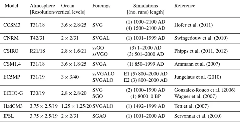
This analysis considers 26 forced climate simulations of the last millennium produced with 8 different AOGCMs: CCSM3, CNRM-CM3.3 (CNRM hereafter), CSM1.4, CSIRO Mk3L 1.2 (CSIRO hereafter), ECHAM5/MPIOM (EC5MP hereafter), ECHO-G, HadCM3 and IPSLCM4 (IPSL hereafter) (see Table 1 for general details and references therein).
These simulations have been developed during the last decade and constitute the currently available AOGCM simu-lations for the last millennium, prior to the ongoing CMIP5– PMIP3 experiments (Schmidt et al., 2011, 2012; Braconnot et al., 2012). The ensemble has been built by incorporating all AOGCM experiments presented in Jansen et al. (2007), except for the Stendel et al. (2005) simulation of the last 500 years with the ECHAM4/OPYC3 model, plus all AOGCM runs developed between then and the beginning of the co-ordinated CMIP5–PMIP3 effort. The ensemble is therefore heterogeneous in terms of forcing configurations and initial conditions, since the simulations were produced with differ-ent AOGCMs. Further and most importantly, differdiffer-ent
ex-ternal forcing boundary conditions were used, depending on the institutions that carried out the simulations and succes-sive updates of the forcing estimates that progressucces-sively be-came available (see Sect. 3). The variety of forcing factors and forcing reconstructions considered herein complement those used for the CMIP5–PMIP3 experiments, by consider-ing some estimations not included in Schmidt et al. (2011, 2012). This will allow exploration of a larger spectrum of plausible scenarios for the last millennium and, in some in-stances, assessment of the degree to which the agreement be-tween simulated and reconstructed responses is modified by different specifications of the same forcing. This analysis fo-cuses on the last 12 centuries (800–2000 AD). A description of the general details for each simulation involved herein, including horizontal resolution, number of atmospheric and oceanic levels, the set of external forcings considered and the exact period of simulation, is included in Table 1. The shorter simulations (the 550-yr HadCM3 and CCSM3 runs) are used in some parts of this study, while the longer runs (the 8-kyr ECHO-G and the 2-kyr CSIRO simulations) are only considered after 800 AD.
Given the number of models involved in this analysis, an in-depth description of each one is outside the scope of this paper. The reader is guided to references in Table 1 for that purpose. Six out of the eight models are effectively differ-ent AOGCMs, whereas the ECHO-G and the CCSM1.4 are earlier versions of the EC5MP and CCSM3 models, respec-tively. Some of the simulations (CCSM3, CSM1.4, CNRM, HadCM3) have been corrected for climate drift by estimating long-term trends from available pre-industrial control runs.
3 External forcing factors
Table 1. Models and experiments considered for the analysis (column 1), the resolution and number of levels in their atmospheric (column
2) and oceanic (column 3) components, the set of external forcings considered in the experiment configuration (column 4), the period of simulation (column 5) and the original reference describing the experiments (column 6). Legend for external forcing: (S) solar forcing using stronger changes in amplitude (i.e. larger than 0.2 % TSI change from the LMM to the present); (ss) solar forcing using weaker changes in amplitude (i.e. lower than 0.1 % TSI change from the LMM to the present; (V) volcanic activity; (G) greenhouse gases; (A) anthropogenic aerosols; (L) land use changes and (O) orbital variations.
Model Atmosphere Ocean Forcings Simulations Reference [Resolution/vertical levels] [(no. runs) length]
CCSM3 T31/18 3.6×2.8/25 SVG (1) 1000–2100 AD Hofer et al. (2011) (4) 1500–2100 AD
CNRM T42/31 2×2/31 SVGAL (1) 1001–1999 AD Swingedouw et al. (2010)
CSIRO R21/18 2.8×1.6/21 ssGO (3) 1–2000 AD Phipps et al. (2011, 2012) ssVGO (3) 501–2000 AD
CSM1.4 T31/18 3.6×1.8/25 SVGA (1) 850–1999 AD Ammann et al. (2007)
EC5MP T31/19 3×3/40 ssVGALO E1 (5) 800–2000 AD Jungclaus et al. (2010) SVGALO E2 (3) 800–2000 AD
ECHO-G T30/19 2.8×2.8/20 SVG (2) 1000–1990 AD Gonz´alez-Rouco et al. (2006) SGO (1) 8000–0 BP Wagner et al. (2007) HadCM3 3.75×2.5/19 1.25×1.25/20 SVGALO (1) 1492–1999 AD Tett et al. (2007) IPSL 3.75×2.5/19 2×2/31 SGAO (1) 1001–2000 AD Servonnat et al. (2010)
through the last millennium, respectively (Jungclaus et al., 2010, see Sect. 3.1).
This section illustrates and compares the main differences between the various forcing estimations shown in Fig. 1. See also Table 2 for the original references of the source reconstructions used with each model for natural forcings and well-mixed GHGs. The text will be organized herein into natural (Sect. 3.1) and anthropogenic (Sect. 3.2) forcing factors. In the case of GHGs, these will be included in the group of anthropogenic forcings, even if most contributions to their global variability before 1850 AD may be of natural origin. The same exception applies to land use. Additionally, in Sects. 5 and 6, a total external forcing expressed in radia-tive forcing units is obtained for each model integrating all natural and anthropogenic contributions for the purpose of a better comparison among the various forcing configurations, simulations and reconstructions (Sect. 3.3).
3.1 Natural forcing
Solar irradiance changes can play a major role in forcing decadal to centennial variability through the last millennium (e.g. Crowley, 2000; Zorita et al., 2005). The amplitude of its variations is nowadays estimated to be much smaller (e.g. Lean et al., 2002; Foukal et al., 2004; Solanki and Krivova, 2004; Wang et al., 2005; Krivova et al., 2007; Gray et al., 2010) than previous published estimates (e.g. Hoyt and Schatten, 1993; Lean et al., 1995; Bard et al., 2000). Yet, a recent reconstruction (Shapiro et al., 2011) still endorses
large background variations in irradiance (see discussion in Schmidt et al., 2011, 2012).
Radiative forcing (W/m 2)
260 280 300 320 340 360
380 800 1000 1200 1400 1600 1800 2000
CO
2
estimations (ppmv)
-0.5 0 0.5
1 1.5
2 2.5
-0.5 0 0.5
1 1.5
2 2.5
800 1000 1200 1400 1600 1800 2000
Anthropogenic forcing (W/m
2)
Year Year
a)
e) b)
c)
d) CSM1.4
CCSM3
EC5MP-E1 EC5MP-E2
ECHO-G
IPSL
CNRM
CSIRO
HadCM3
-1 -0.5 0 0.5 1 1.5 2 2.5
3 800 1000 1200 1400 1600 1800 2000
Solar + anth. forcing (W/m
2)
Year
-20 -15 -10 -5 0 5
800 1000 1200 1400 1600 1800 2000
Total external forcing (W/m
2)
Year -1.5
-1 -0.5 0 0.5
1 1.5
2
Total external forcing (W/m
2)
31-yrs low pass filter, wrt 1500-1850 AD
g)
h) f)
-4 -3 -2 -1 0 1 2 3 4 5
TSI anomalies (W/m
2)
Schmidt et al. 2011 Shapiro et al. 2011
1362 1364 1366 1368
TSI 1500-1850 AD (W/m
2)
-15 -10 -5 0 -5 -10
800 1000 1200 1400 1600 1800 2000
Volcanic forcing (W/m
2)
Year
800 1000 1200 1400Year 1600 1800 2000
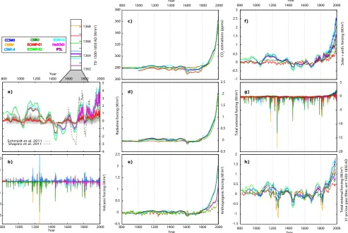
Fig. 1. Estimations of external forcings used to drive the simulations in Table 1 (see labels). The reference period for all panels showing
anomalies is 1500–1850 AD. (a) TSI anomalies. The CMIP5–PMIP3 recommended solar forcing (Schmidt et al., 2011) and the reconstruction from Shapiro et al. (2011) are also shown for comparison. The inset shows TSI averages for the reference period. (b) Volcanic forcing estimations in radiative forcing units. Note: the volcanic forcing is always negative. The orientation above or below the x-axis is arbitrary and only for clarity in the display. (c) CO2concentrations (ppmv). Values from the EC5MP are diagnosed online and correspond here to 31-yr filtered outputs of the ensemble averages. (d) Equivalent CO2forcing (Wm−2) including well-mixed GHGs. Note that the CNRM and IPSL models depict identical values. (e) Anthropogenic forcing (Wm−2) including the contributions of GHGs, aerosols and land use.
(f) Estimations of external forcing including anthropogenic and solar contributions. (g) Estimations of TEF adding anthropogenic and natural
contributions. (h) 31-yr moving average filtered outputs of anomalies in (g). All radiative forcing units are Wm−2. Note: IPSL does not include volcanic forcing; for the ECHO-G and CSIRO models, estimations of TEF correspond to the simulations with volcanic forcing. Dashed lines for the CNRM, CSM1.4, EC5MP and HadC3M in panels (e)-(h) indicate approximations (see text for details).
The STSI group clusters with an increase in TSI larger than 0.23 % from the LMM to the present and a decrease of more than 0.17 % from the Medieval Maximum to the LMM. The EC5MP and ECHO-G show the largest percentage of change in the transition from the LMM–present as is also evidenced in Fig. 1a. The ssTSI group displays a reduction of 0.04 % during the Medieval to LMM transition and an increase of less than 0.09 % from the LMM to the present.
The coherent evolution within the STSI solar forcing stems from the use of a single record of production rates of the cosmogenic isotope10Be in Antarctic ice cores from Bard et al. (2000). The CSM1.4 and the EC5MP-E2 ensemble use the original values provided by Bard et al. (2000) (note that series overlap in Fig. 1a) and do not include estimations of
the 11-yr solar cycle. In turn, the CCSM3, CNRM, ECHO-G, HadCM3 and IPSL simulations use a version of the Bard et al. (2000) record spliced by Crowley (2000) to a reconstruc-tion of TSI (Lean et al., 1995) based on the sunspot record of solar activity since 1610 AD. Therefore, all these records in-clude an estimate of the 11-yr solar cycle since this date. The slightly different forcings adopted by the various AOGCMs are due to different calibration of the net radiative forcing data provided by Crowley (2000) to the original TSI values of Lean et al. (1995).
Table 2. Reconstructions of natural forcing and well-mixed GHG reconstructions applied to each model in Table 1. Key for labels: Amma03
(Ammann et al., 2003), Bard00 (Bard et al., 2000), Batt96 (Battle et al., 1996), Blun95 (Blunier et al., 1995), Crow00 (Crowley, 2000), Crow03 (Crowley et al., 2003), Crow08 (Crowley et al., 2008), Crow12 (Crowley and Unterman, 2012), Ether96 (Etheridge et al., 1996), Ether98 (Etheridge et al., 1998), Fluck02 (Fluckiger et al., 2002), Gao08 (Gao et al., 2008), Johns03 (Johns et al., 2003), Kriv07 (Krivova et al., 2007), Lean95 (Lean et al., 1995), Marl03 (Marland et al., 2003), McFM06 (MacFarling Meure et al., 2006), Stein09 (Steinhilber et al., 2009).
Model Solar Volcanic CO2 CH4 N2O
CCSM3 Bard00 Amma03 Ether96 Blun95 Fluck02 Lean95
CNRM Bard00 Amma03 McFM06 Blun95 Fluck02 Lean95
CSIRO Stein09 Gao08 McFM06 McFM06 McFM06 CSM1.4 Bard00 Amma03 Ether96 Blun95 Fluck02
EC5MP-E1 Kriv07 Crow08 Diagnosed McFM06 McFM06 Crow12 Marl03
EC5MP-E2 Bard00 Crow08 Diagnosed McFM06 McFM06 Crow12 Marl03
ECHO-G Bard00 Crow00 Ether96 Ether98 Batt96 Lean95
HadCM3 Bard00 Crow03 Johns03 Johns03 Johns03 Lean95
IPSL Bard00 —- McFM06 Blun95 Fluck02 Lean95
Table 3. Percentage of TSI change between the period with highest
TSI values (1130-1160) in the Medieval Maximum and the LMM, and from the LMM to the late 20th century. Percentages are calcu-lated with reference to the LMM average. Note: a 0.25 % change between the LMM and late 20th century is equivalent to a variation of the TSI between the two periods of∼3.4 W m2.
Medieval LMM–late Maximum–LMM 20th century
Model (%) (%)
CCSM3 −0.27 0.23
CNRM −0.18 0.25
CSIRO −0.04 0.05
CSM1.4 −0.17 0.24
EC5MP-E1 −0.04 0.09 EC5MP-E2 −0.27 0.24
ECHO-G −0.22 0.29
HadCM3 – 0.25
IPSL −0.18 0.25
Shapiro et al. (2011) – 0.44
Solanki, 2008). The reconstructed 11-yr cycle is extended before the 17th century by artificially superimposing the av-erage 11-yr solar cycle between 1700 AD and the present. The CSIRO simulations use a10Be-based reconstruction by
Steinhilber et al. (2009) with no 11-yr cycle. None of the sim-ulations consider stratospheric photochemistry and ozone in-teractions (Shindell et al., 2001). Estimations of variability in solar wavelengths (Haigh et al., 2010) are also not included. Figure 1a also shows the TSI reconstructions suggested by Schmidt et al. (2011) to serve as boundary conditions for the CMIP5–PMIP3 last millennium simulations. Figure 1a shows additionally the recent reconstruction of Shapiro et al. (2011) that estimates TSI changes of larger amplitude than any of the reconstructions discussed above (see Table 3). Such variability is difficult to reconcile with the solar forc-ing estimations in Schmidt et al. (2011) and with compar-isons of climate reconstructions with simulations using the Climber-3αEMIC driven by the Shapiro et al. (2011) esti-mates (Feulner, 2011). Nevertheless, this solar forcing recon-struction may be useful for sensitivity modelling experiments (see Schmidt et al., 2012).
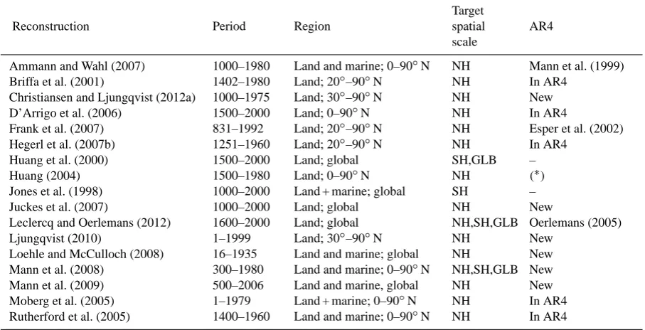
Table 4. Climate reconstructions used in this work. For each record, the temporal extension (column 2) and spatial coverage (column 3)
are shown. Column 4 indicates the spatial scale (NH, SH, GLB) that the reconstruction was used for in Fig. 3. For the NH reconstructions, column 5 indicates if a reconstruction was used in Jansen et al. (2007), or if it is a new record. If the reconstruction substitutes a record used in Jansen et al. (2007) , then the reference of the replaced record is indicated. Notes: resolution is annual for all reconstructions except for Ljungqvist (2010), which is provided in decadal values; in the case of Mann et al. (2008) two reconstructions, the CPS and the EIV method, are considered.(∗)In AR4 Pollack and Smerdon (2004) was considered. Instead, the reconstruction provided in Huang (2004) has been selected herein because it includes high-frequency variability that will be useful for the analysis in Sect. 6.
Reconstruction Period Region
Target spatial scale
AR4
Ammann and Wahl (2007) 1000–1980 Land and marine; 0–90◦N NH Mann et al. (1999) Briffa et al. (2001) 1402–1980 Land; 20◦–90◦N NH In AR4
Christiansen and Ljungqvist (2012a) 1000–1975 Land; 30◦–90◦N NH New D’Arrigo et al. (2006) 1500–2000 Land; 0–90◦N NH In AR4
Frank et al. (2007) 831–1992 Land; 20◦–90◦N NH Esper et al. (2002) Hegerl et al. (2007b) 1251–1960 Land; 20◦–90◦N NH In AR4
Huang et al. (2000) 1500–2000 Land; global SH,GLB – Huang (2004) 1500–1980 Land; 0–90◦N NH (∗)
Jones et al. (1998) 1000–2000 Land + marine; global SH – Juckes et al. (2007) 1000–2000 Land; global NH New
Leclercq and Oerlemans (2012) 1600–2000 Land; global NH,SH,GLB Oerlemans (2005) Ljungqvist (2010) 1–1999 Land; 30◦–90◦N NH New
Loehle and McCulloch (2008) 16–1935 Land and marine; global NH New Mann et al. (2008) 300–1980 Land and marine; 0–90◦N NH,SH,GLB New Mann et al. (2009) 500–2006 Land and marine, global NH New Moberg et al. (2005) 1–1979 Land + marine; 0–90◦N NH In AR4 Rutherford et al. (2005) 1400–1960 Land and marine; 0–90◦N NH In AR4
Orbital forcing is globally small during the last millen-nium but potentially important for seasonality changes at high latitudes (Kaufman et al., 2009). Only CSIRO, IPSL, HadCM3 and one of the ECHO-G simulations include these changes following Berger (1978), and Laskar et al. (2004) in the case of the IPSL model. EC5MP follows Bretagnon and Francou (1988) for orbital changes and additionally considers nutation.
Volcanic forcing is included in all simulations except for the IPSL, the 8000-yr ECHO-G run and 3 simulations of the CSIRO model (Table 1). The various estimations of vol-canic forcing are shown in Fig. 1b, in radiative forcing units. CCSM3 and CNRM originally incorporate this forcing in aerosol optical depth values, and their conversion into ra-diative forcing units has been done following Hansen et al. (2002), where a factor of −21 W m−2 is suggested for the conversion. This value is within the range of estimations made also by Wigley et al. (2005).
The reconstructions of stratospheric aerosols from vol-canic eruptions are based on ice core data from Antarctica and Greenland. The derived time series of volcanic forc-ing tend to display consistent timforc-ing for major eruptions (Fig. 1b). However, they often present differences on the magnitudes of individual events. Our knowledge of volcanic forcing over the past millennium is poorly constrained,
par-ticularly in regard to the strengths of individual eruptions (Forster et al., 2007; Schmidt et al., 2011).
The implementation of volcanic forcing into AOGCMs was done only by including the net effect of stratospheric volcanic aerosols on the global radiation balance (ECHO-G, CSIRO) or latitudinally resolved changes in optical depth in the stratosphere (EC5MP, HadCM3). These differences may have an impact on the climatic effects in the aftermath of volcanic eruptions on the atmospheric circulation, espe-cially over the extratropical hemispheres during wintertime (e.g. Robock, 2000; Fischer et al., 2007). Although volcanic impacts are restricted to a few years, the temporal clustering of volcanic outbreaks may also have impacts beyond these time scales (see Sect. 5).
parametrizations. The CMIP5–PMIP3 volcanic forcing stan-dards for last millennium simulations will rely on the most recent reconstructions (Crowley et al., 2008; Gao et al., 2008; Crowley and Unterman, 2012). Comparison and details are given by Schmidt et al. (2011).
3.2 Anthropogenic forcing
Estimates of the concentration changes of the main well-mixed GHGs (CO2, CH4 and N2O) are obtained from
Antarctic ice cores (Forster et al., 2007; Joos and Spahni, 2008). The records used to produce the simulations in Ta-ble 1 were selected according to the availability of data at the time of production of model experiments. The CO2
concen-trations were prescribed in each model (Fig. 1c) except for the EC5MP, which calculates it interactively (see Jungclaus et al., 2010). Figure 1d shows an estimation of the GHG ra-diative forcing obtained from the concentrations of the three GHGs in each model following Myhre et al. (1998). This al-lows the comparison of the total effect of CO2, CH4and N2O
between different simulations, and later with other anthro-pogenic and natural forcings.
HadCM3 used estimated changes in GHGs only in the in-dustrial period; values after 1750 AD were taken from Johns et al. (2003), and constant pre-industrial values were as-sumed before this date. The ECHO-G model used last mil-lennium reconstructions from Etheridge et al. (1996) for CO2
and from Etheridge et al. (1998) for CH4; Battle et al. (1996)
estimates for N2O were included after 1850 AD and assumed
constant before. CSM1.4 and CCSM3 used reconstructions from Etheridge et al. (1996) for CO2, Blunier et al. (1995)
for CH4, and Fluckiger et al. (2002) for N2O. All
simula-tions from the last three models use different spline interpo-lations to obtain annual concentration values. In addition to the different origin of the data, the different interpolation ap-proaches produce variability in the evolution of pre-industrial concentrations and forcings in Fig. 1c, e. The CSIRO runs used values derived from updated reconstructions provided by MacFarling Meure et al. (2006). CNRM and IPSL incor-porate also estimations of MacFarling Meure et al. (2006) for CO2. However, transient changes in CH4 and N2O
concen-trations are considered only after 1850 AD and taken from Blunier et al. (1995) and Fluckiger et al. (2002), respectively. Before this date the concentrations are kept constant. These pre-1850 AD concentration values are higher than those sug-gested by MacFarling Meure et al. (2006). Thus the CO2
con-centrations in the CNRM and IPSL simulations were lowered by about 5 ppmv to compensate for the relatively high CH4
and N2O levels. This can be appreciated in the lower CO2of
CNRM/IPSL in Fig. 1c, while in Fig. 1d the GHG forcing of CSIRO, CNRM and IPSL co-vary in phase.
CO2and GHGs forcing evolve very similarly for all
simu-lations that prescribed GHG concentration values in Fig. 1c, d. Excluding arbitrary changes produced by spline interpola-tions, the multicentennial changes displayed by the various
forcings are due to natural feedbacks from the ocean and ter-restrial biosphere in response to variations in climate; addi-tional effects of land cover change are also possible (Pon-gratz et al., 2010). The diagnosed ensemble averages of CO2
concentrations simulated by EC5MP (Fig. 1c) are below the MacFarling Meure et al. (2006) observations in the 20th cen-tury. This discrepancy is arguably due to an underestimation of the emissions related to land use change, among other fac-tors discussed in Jungclaus et al. (2010). The pre-industrial CO2concentration values show more variability in the E2
en-semble, albeit with changes of somewhat smaller magnitude than in the MacFarling Meure et al. (2006) reconstruction. The larger variability in the E2 (relative to the E1) ensemble may be related to its slightly larger temperature fluctuations (see Sect. 5), with higher values during the MCA and lower during the LIA. The smaller number of members in E2 (3) relative to E1 (5) may also have contributed to this effect, with less chances of cancelling out deviations associated with internal variability among ensemble members. The observed minimum in the 17th and 18th centuries is not reproduced.
NCAR model, which is well within the range of the values estimated herein for the CSM1.4 model (Dai et al., 2001).
Land use changes are considered through the whole pe-riod of interest in Fig. 1e in the EC5MP simulations. The radiative forcing associated with these land use changes was calculated off-line using the radiative code of the ECHAM5, thus including only the albedo effect (Jungclaus et al., 2010); it causes a long-term cooling that adds to that of aerosol forc-ing (Pongratz et al., 2009, 2010). The land use forcforc-ing used in the HadCM3 and the CNRM simulations after the 18th century was not available and hence not considered in sub-sequent analyses, even when the effect of this forcing during the 19th and 20th century may still be non-negligible (Bauer et al., 2003).
On the basis of the previous description, the total anthro-pogenic forcing illustrated in Fig. 1e accurately represents the actual forcings used in the model simulations over the whole millennium for the CCSM3, CSIRO, ECHO-G and IPSL, and for the CNRM, CSM1.4, EC5MP and HadCM3 until the 19th century; thereafter, these forcing estimations are subjected to the approximations and limitations described above (dashed lines in Fig. 1e).
During pre-industrial times all simulations where CO2
concentration was prescribed display a very similar evolu-tion of the total anthropogenic forcing. EC5MP shows less low-frequency variability during this period. In the 20th cen-tury the models in which the only anthropogenic forcings are GHGs (CCSM3, CSIRO and ECHO-G) are also, as ex-pected, the ones showing the largest increase in total forc-ing. According to the approximations shown in Fig. 1e, the other simulations gradually decrease, with the EC5MP an-thropogenic forcing being the lowest during the 20th cen-tury. The resulting temperature response in each model will be built upon the balance of this anthropogenic effect on forc-ing, the effect of natural forcings displayed in Fig. 1a, b and the climate sensitivity of each model.
3.3 Total external forcing
The addition of the natural and anthropogenic forcings con-sidered in Sects. 3.1 and 3.2 builds a total external forcing (TEF hereafter) for each model as shown in Fig. 1f–h. The use of TEF helps us to better understand the temperature re-sponse of the models described in Sect. 5 and the assessment of climate sensitivity developed in Sect. 6.
Figure 1f shows the sum of anthropogenic forcing in Fig. 1e and solar forcing, thus excluding the volcanic con-tribution. Figure 1g shows TEF by adding also the effect of volcanic forcing. For comparison with the analysis in the fol-lowing sections, Fig. 1h shows 31-yr filtered outputs of TEF expressed as anomalies relative to 1500–1850 AD. Forcing changes in the pre-industrial period are dominated by so-lar and volcanic activity. The comparison of the IPSL TEF, for which volcanic forcing is not included, with that of the other models (see Fig. 1h) serves as an illustration of the
1e-06
1e-05 0.0001 0.001 0.01 0.1 1
Spectral Density
1e-06 1e-05 0.0001 0.001 0.01 0.1 1
Spectral Density
1e-06 1e-05 0.0001 0.001 0.01 0.1 1
200 100 50 20 10 5 2
Spectral Density
Period (yrs) CSM1.4
CCSM3
EC5MP-E1 EC5MP-E2
ECHO-G IPSL
CNRM CSIRO HadCM3
200 100 50 20 10 5 2
Period (yrs)
b) a)
c)
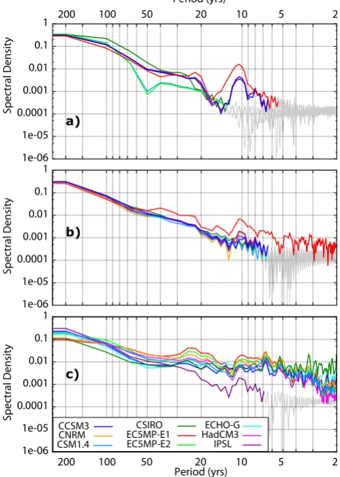
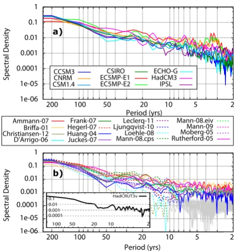
Fig. 2. Normalized spectra for various combinations of external
forcing: (a) solar forcing (Fig. 1a); (b) solar and anthropogenic forc-ing (see Fig. 1f); (c) all natural and anthropogenic forcforc-ings (TEF; see Fig. 1g). Grey lines correspond to frequency bands affected by Gibbs oscillations (see text for details). For the sake of clar-ity, spectral curves corresponding to AR1 processes are not shown. Note: IPSL does not include volcanic forcing; for the ECHO-G and CSIRO models, estimations of TEF correspond to the simulations with volcanic forcing.
frequency domain is displayed for several of the forcing com-binations in Fig. 1. Figure 2a shows spectra for the various solar forcing configurations (Fig. 1a). The estimation of these spectra are somewhat burdened by the fact that solar forc-ing specifications do not have variability at high frequen-cies, which produces Gibbs oscillations in this part of the spectrum (grey lines, Bloomfield, 1976) and precludes for this case a clear comparison of the relative contribution to total variance of low and high frequencies. However, this is useful as an illustration of the relative importance of the variance accumulation at decadal timescales, and for com-parison with other forcings in Fig. 2. CSM1.4, CSIRO and EC5MP-E2 forcings do not include an 11-yr solar cycle sig-nal and thus do not show any contribution to variance cen-tred around the 11-yr band. Their spectra suffer from Gibbs oscillations below the 20-yr timescale. This problem is re-duced in the other simulations that do consider an 11-yr solar cycle. In the case of EC5MP-E1, this variability is imposed through the whole millennium, thus showing maximum vari-ance at these frequencies. CNRM, ECHO-G, HadCM3 and IPSL use the 11-yr variability in the last few centuries (see Sect. 3.1). This is reflected in an overlap of their spectra at these timescales, albeit showing a smaller proportion of vari-ance than EC5MP-E1. It is also interesting to note the rela-tive increases of variability from the 20- to 40-yr timescales. Figure 2a can be compared with Fig. 2b which shows the sum of solar and anthropogenic forcings. Here, the propor-tion of variability accounted for by the 11-yr solar cycle is importantly diminished and only noticeable in the EC5MP-E1 case. The radiative forcing associated with the land use changes in the EC5MP introduces variability at high and low frequencies (Jungclaus et al., 2010; Fig. 1a), thereby con-tributing to avoidance of Gibbs oscillations in the EC5MP spectra of anthropogenic forcing (red line in Fig. 2b).
Figure 2c shows spectra for TEF (Fig. 1g). Two features are prominent. Firstly, the relative contribution of the 11-yr solar cycle has been greatly diminished in all cases. This suggests that only a small simulated global or hemispheric signal, at this frequency, is to be expected in the model re-sponse for the last millennium. Additionally, the proportion of variance from interannual to multidecadal timescales, up to 40-yr periods, is increased in comparison to Fig. 2a, b. This is arguably due to the multidecadal variability associated with the occurrence of large volcanoes. An exception here is the IPSL case, which does not include volcanic forcing and serves as a reference that can be compared with the other spectral curves. For longer timescales, the simulations that show relatively lower contributions to variance are the ssTSI group (EC5MP-E1 and CSIRO) and the CNRM forcing. For CNRM this may be due to the relatively higher proportion of high-frequency variability due to volcanic activity (this is the simulation with highest volcanic forcing in Fig. 1b) and the somewhat intermediate trends in TEF amplitude (Fig. 1g, h).
4 Hemispheric and global reconstructed temperatures
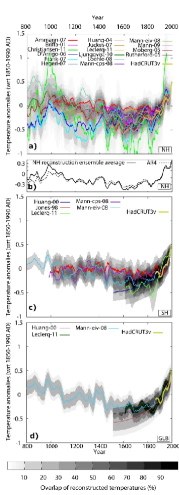
This section presents the set of hemispheric and global re-constructions considered in this study to update and dis-cuss new evidence since Jansen et al. (2007). These recon-structions (Table 4) will be compared with the simulations and forcing estimates in the following sections. The criteria for including a reconstruction in Table 4 was that it used a new methodological approach or new data relative to exist-ing ones. Some reconstructions that were considered to be superseded by new versions were not included in the data set. This is the case, for instance, of the Mann et al. (1999) reconstruction that was omitted in favour of an improved version provided by Ammann and Wahl (2007), or the case of Esper et al. (2002) which has been superseded by Frank et al. (2007). All reconstructions in Table 4 have a minimum length of four centuries and in some cases start well before 800 AD, the beginning of the simulations considered here (column 2). The time resolutions are annual for all recon-structions except for Ljungqvist (2010), which has decadal resolution. Even if records have annual resolution, this may not represent the real time resolution, for instance, in the case of borehole data (Huang et al., 2000) that provide in-formation on multicentennial trends. This also occurs with some other reconstructions in the table that show low vari-ance on interannual timescales despite the data being pro-vided at annual resolution (Briffa et al., 2001; Hegerl et al., 2007b; Loehle, 2007; Mann et al., 2009; Leclercq and Oer-lemans, 2012; Christiansen and Ljungqvist, 2011). Season-ality biases may also be present, particularly in summer due to the important contribution of tree ring data (Jones et al., 2009). The group of reconstructions is heterogeneous not only from the time domain perspective. Different reconstruc-tions use proxy information from different regions and were developed from different land and ocean spatial coverages (column 3). The majority of them target NH temperatures, but some of them aim to reconstruct Southern Hemisphere (SH) and/or Global (GLB) scale temperatures (column 4). This will allow the state of knowledge at these spatial scales to be illustrated and compared. Column 5 in Table 4 indicates whether a given record had already been considered in AR4 (Jansen et al., 2007).
The present ensemble includes 16 reconstructions for the NH, out of which 7 are new records and 3 are updates or improved versions of their AR4 counterparts (see Ta-ble 4). Therefore, this assessment provides new evidence that leans on new data, methods or updates that improve previous versions.
account their uncertainties as in Jansen et al. (2007). For each year, the temperature axis is divided into 0.01◦C pixels that receive a score of 1 (2) if they lie within the range of the reconstructed temperatures±1.645 (±1) standard deviation. The scores are summed over all reconstructions considered and scaled to range within 0 and 100 % of overlap. The re-sulting uncertainty distribution is the basis for the model– data comparison in Sect. 5.1. Contributions to the spread stem not only from uncertainties in proxy data but also from various other sources, including (Jansen et al., 2007; Jones et al., 2009) the different reconstruction methods; the diver-sity of data and periods used in the calibration process; the different proxy data sets that in some cases overlap and in others bring information from various source regions, the land or marine character of the source locations; and the dif-ferent seasonalities. These limitations should be kept in mind in the comparison with model simulations discussed below, as well as in the evaluation provided in Sect. 6.
Figure 3a shows a qualitative agreement among the re-constructions. The display depicts a warm MCA followed by a colder LIA and a subsequently warmer instrumen-tal period. Temperatures in the first half of the 20th cen-tury are comparable to those in the MCA, but instrumen-tal measurements in the last decades of the millennium are above those of any reconstruction since the MCA. How-ever, some differences with AR4 are caused by two recon-structions: Christiansen and Ljungqvist (2012a) and Loehle and McCulloch (2008). The extratropical NH reconstruction of Christiansen and Ljungqvist (2012a) (Fig. 5 in their pa-per) displays larger low-frequency amplitude changes than any other reconstruction in the ensemble, noticeably en-larging the spread during the MCA and mid-20th century. As in the case of Christiansen and Ljungqvist (2011), re-constructions using the LOC method aim to preserve low-frequency variability, perhaps to the detriment of high fre-quencies (Christiansen, 2011). An overestimation of variabil-ity can not be ruled out, and some studies suggest these re-constructions may be taken as an estimation of maximum bounds for low-frequency amplitude changes during the last millennium (Tingley and Li, 2012; Moberg, 2012; Chris-tiansen, 2012; Christiansen and Ljungqvist, 2012b). This re-construction shows noticeably more variance at low frequen-cies not only in the pre-industrial period but also during the 20th century. The corrected non-tree ring reconstruction of Loehle and McCulloch (2008) shows noticeably larger tem-perature anomalies during medieval times than at present and reaches values larger than late 20th-century observations during the 9th century.
As a noticeable difference with AR4, this ensemble shows greater multicentennial variability. This is illustrated in Fig. 3b where the ensemble average for AR4 and for this study are compared. The new ensemble average in Fig. 3b shows larger differences between the MCA and the LIA. These differences, however, fall within the envelope of un-certainty and therefore cannot be regarded as a significantly
Fig. 3. NH (a, b), SH (c) and GLB (d) temperature anomalies wrt
different evolution of last millennium temperatures from this perspective. However, the new ensemble average has 1.55 times more variance than the AR4 average (1.81 times more variance for the 31-yr filtered series shown in Fig. 3b). This increase is significant based on an F-test with a significance levelα= 0.05 (also accounting for the loss of degrees of free-dom in the filtered version). An important part of this en-hancement of low-frequency variability is due to the con-tribution of the Christiansen and Ljungqvist (2012a) curve. If this is not included in the evaluation, raw data variances are significantly increased by a factor of 1.23 (α=0.05), whereas the low-frequency amplification of variability (1.33) is significant only at theα=0.21 level.
Figure 3c, d show similar plots for the SH and GLB scales. Some notes of caution are pertinent. These panels are shown for the sake of illustration of the present stage of information at these spatial scales, but the estimation of their uncertainty bounds is limited by the very few reconstructions available. For the SH, the five existing records reflect very similar mul-ticentennial trends, whereas multidecadal variability can be quite different among the records. It should be kept in mind that three of the records considered share identical or over-lapping proxy information or use comparable methods as in the case of the CPS approach (Jones et al., 1998; Mann et al., 2008). The evidence shown in Fig. 3c is suggestive of rela-tively higher temperatures before the 15th century, compara-ble to those at the beginning of the 20th century, and a colder interval spanning the period between the 15th and 19th cen-turies. The last decades show values above the reconstruc-tions during the whole period.
At a global scale, only three records are available (Fig. 3d): a borehole reconstruction (Huang et al., 2000), a glacier record (Leclercq and Oerlemans, 2012), and a multiproxy reconstruction (Mann et al., 2008); only the latter of these reconstructions goes back in time beyond 1600 AD (Mann et al., 2008). The amplitude of changes over the last 400 yr is in broad agreement among the three records.
5 Hemispheric and global simulated temperatures: model–data consistency
This section provides an analysis of the simulated temper-ature response in comparison to the forcings described in Sect. 3. The response of the simulations listed in Table 1 is also compared to available information from the last mil-lennium climate reconstructions presented in Sect. 4. Sec-tion 5.1 assesses the millennial temporal evoluSec-tion in the reconstructions and simulations. Section 5.2 explores the spatial detail of the transition from the MCA to the LIA.
5.1 Temporal evolution
Figure 4 shows hemispheric and global temperature anoma-lies with respect to the period 1500–1850 AD for the suite of
Fig. 4. NH (a, b), SH (c) and GLB (d) simulated temperature
simulations listed in Table 1. The reason for this choice in-stead of the 1850–1990 AD period used for reconstructions (Fig. 3) is that during 1850–1990 AD the various simulations use different forcings (see Sect. 3), and therefore their trends during this period are not comparable and render this time interval as invalid as a common reference for model simu-lations. Additionally, the choice of a longer period (e.g. the whole millennium) is precluded by the fact that some of the simulations in Table 1 only span the last 500 yr. Thus, the choice of 1500–1850 AD as a reference secures a period of data availability for all the simulations and in which the forc-ings applied were similar. The grey background shading rep-resents the spread of the reconstructions using this reference period and is calculated as in Fig. 3. Note, however, that the spread changes from Fig. 3 to Fig. 4. Due to the choice of a different reference period in this figure, the grey shading is somewhat narrower during the 1500–1850 AD interval and slightly wider over the rest of the millennium relative to what is shown in Fig. 3. Hence, care must be taken not to interpret the spread in Fig. 4 as a measure of the reconstruction ensem-ble uncertainty of past temperature changes. The shape of the spread can be used for the purpose of a qualitative compar-ison of agreement or disagreement between simulations and reconstructions.
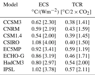
Figure 4a shows results for the NH. As in the case of the reconstructions, the simulations show the sequence of tem-perature stages discussed above, i.e. higher temtem-peratures in the MCA and industrial period and a relative minimum in the LIA. For the sake of clarity, Fig. 4b shows the reconstruction ensemble average (Fig. 3b) plotted together with the average across all simulations available for each model with an iden-tical forcing configuration. In spite of the relative differences among the inter-model forcing configurations, the trajectory of all simulations shows a high degree of similarity. Most of the simulations show minima during the Wolf, Sp¨orer, Maun-der and Dalton intervals, albeit modulated by the presence of volcanic activity for those simulations that incorporate it. The simulations showing less low-frequency variability dur-ing pre-industrial times are the ssTSI group, comprisdur-ing the EC5MP-E1 and the CSIRO ensembles, whereas the STSI group shows larger changes in amplitude. Overall, the simu-lated trajectories follow closely the TEF in Fig. 1h. The dis-tribution of warming trends in the last two centuries of the simulations follow also a similar arrangement in spite of the limitations discussed regarding the estimation of TEF. The largest temperature increases are simulated by the runs incor-porating only GHGs and natural forcing, and decreasing ac-cording to the inclusion of additional factors (aerosols, land use; see Sect. 3) that contribute with negative forcing during this period. The 20th-century trends are, however, not solely a function of the applied external forcing but also of model sensitivity. As a mean of complementary information, Ta-ble 5 shows values of equilibrium climate sensitivity (Schnei-der et al., 1980) and transient climate response (Knutti et al., 2005) for the various models in Table 1. Both quantities serve
Table 5. Equilibrium climate sensitivity (ECS) and transient
cli-mate response (TCR) esticli-mates for the different models. The equiv-alent increase in temperature degrees for a doubling of CO2 is shown between square brackets. Values were extracted from ref-erences in Tables 1 and Solomon et al. (2007). The conversion to
◦C/2×CO
2was done following Houghton et al. (2001)
Model ECS TCR
◦
C/(Wm−2)[◦C/2×CO2] CCSM3 0.62 [2.30] 0.38 [1.41] CNRM 0.59 [2.19] 0.43 [1.59] CSM1.4 0.54 [2.00] 0.39 [1.45] CSIRO 1.08 [4.00] 0.40 [1.50] EC5MP 0.92 [3.41] 0.59 [1.19] ECHO-G 0.86 [3.19] 0.46 [1.71] HadCM3 0.80 [2.97] 0.54 [2.00] IPSL 1.02 [3.78] 0.57 [2.11]
as informative estimates of the general sensitivity of climate against external perturbations and will be used below and in Sect. 6.
between reconstructions and forcings. Although forcing fac-tors over the last millennium are not perfectly constrained (e.g. Plummer et al., 2012; Schmidt et al., 2011), the qual-ity of their reconstructions (Sect. 3) can be considered ho-mogeneous through time, and thus it can be argued that this discrepancy points to a problem in the reconstructions dur-ing this period. For instance, one possibility is that climate reorganizations during medieval times would invalidate the proxy–instrumental relationships during this period (Seager et al., 2007; Graham et al., 2011; Diaz et al., 2011; Trouet et al., 2012), thereby affecting reconstruction quality. If this were the case, the implications would be relevant since this is the period showing the largest temperature anomalies in the last 1200 yr. Thirdly, the simulations showing the largest discrepancies with the reconstruction spread in the 20th cen-tury are the CCSM3, the ECHO-G and the EC5MP ensem-bles. CCSM3 and ECHO-G clearly suffer from not including aerosols and land use, and they overestimate the warming in comparison to the reconstructions. In turn, the EC5MP tem-perature increase is lower than in the reconstructions. The reasons for this are unknown since EC5MP shows, together with HadCM3 and IPSL, one of the highest transient climate responses in future scenario simulations (see Table 5). Ar-guably, the physics related to the treatment of aerosols or land use changes may exacerbate the related cooling in this model during the 20th century.
Figure 4a still shows overall a very similar situation to Fig. 6.13 in AR4 (Jansen et al., 2007). Progress since then is related to the existence of a considerable number of AOGCM simulations compared to the ensemble in AR4, which com-prised only a few AOGCMs and a few EMIC simulations. The ensemble in Fig. 4a shows considerably more variability at multidecadal timescales than the simulations used in AR4 did. This may be related to internal variability in AOGCMs being larger than in EMICs. The response at lower frequen-cies and the amplitude of changes from the MCA to the LIA is larger in the STSI simulations shown in Fig. 4a, b than in the EMIC simulations illustrated in Fig. 6.13 of AR4. Addi-tionally, the qualitative comparison that can be derived from simulations and reconstructions in Fig. 4a, b and 6.13 in AR4 evidences that, irrespective of using AOGCMs or EMICs, the evolution of simulated changes during the last millennium is very similar and suggestive of a linear relation between NH temperatures and TEF applied in each model simulation. Section 6 will introduce a metric that will provide a more quantitative approach to model–data comparison.
Figure 4c, d show the model–data comparison for the SH and GLB averages. Similar conclusions can be reached to those obtained from Fig. 4a, b. The simulations show less spread in the SH than in the NH. Also, trends in the 20th cen-tury are of smaller amplitude. This is consistent with obser-vations and in general with the few reconstructions available. Therefore, the smaller temperature spread in the SH recon-structions (Fig. 3c) may arguably be a realistic feature and not a result of having a small number of reconstructions. The
1e-06 1e-05 0.0001 0.001 0.01 0.1 1
200 100 50 20 10 5 2
Spectral Density
Period (yrs) Ammann-07
Christiansen-12 D’Arrigo-06
Briffa-01 Frank-07
Rutherford-05 Leclerq-11
Ljungqvist-10 Mann-08.cps
Mann-08.eiv
Hegerl-07 Moberg-05
Juckes-07
Mann-09 Loehle-08
Huang-04
b)
1e-06 1e-05 0.0001 0.001 0.01 0.1 1
200 100 50 20 10 5 2
Spectral Density
Period (yrs) CSM1.4
CCSM3
EC5MP-E1 EC5MP-E2
ECHO-G IPSL
CNRM CSIRO HadCM3
a)
0.001 0.0001 0.01 0.1
100 50 20 10 2
HadCRUT3v
Fig. 5. Normalized spectra of simulated (a) and reconstructed
(b) NH temperatures. For the models for which several simulations
(CCSM3,ECHO-G,CSIRO) were available, averages of the runs in-cluding volcanic forcing were considered (Fig. 4). Grey lines depict Gibbs oscillations in reconstructions missing high-frequency vari-ability. The inset in (b) shows the normalized spectra of the NH instrumental data (Brohan et al., 2006).
lower multicentennial variability can be related in the SH to the lower extent of land areas. The comparison of GLB be-tween simulations and reconstructions shows as expected an intermediate situation to that of the NH and SH. It is notewor-thy that in the 9th and 10th centuries the simulations, consis-tent with the TEF (Fig. 1h), are below the Mann et al. (2008) EIV reconstruction.
Some final comments related to specific simulations in the ensemble are pertinent. The dashed blue lines corre-spond to the high values simulated in the 10th and 11th centuries by one of the ECHO-G reconstructions (Gonz´alez-Rouco et al., 2003). These values have been demonstrated to be exceptionally high due to a problem in initial condi-tions (Goosse et al., 2005) and corrected for the NH using an EMIC (Osborn et al., 2006).
timescales) the reconstructions tend to show a somewhat sta-ble level of variance density, whereas most of the simulations (except for EC5MP and CNRM) show a continuous decay. Interestingly, the spectra of TEF show a similar decay for all models except for the CSIRO (Fig. 2) at high frequencies. This suggests either a possible noise contamination at high frequencies on the proxy side or an underestimation of inter-annual variability by the models. The inset in Fig. 5b shows the normalized spectra of the NH instrumental data (Brohan et al., 2006), evidencing a behaviour that is more similar to that of the proxies and thereby suggesting an underestima-tion of interannual variability by the models. Addiunderestima-tionally, some of the simulations (CNRM, EC5MP) show an anoma-lously high accumulation of variability at 3–5-yr timescales which is not visible in the reconstructions. This is produced in these models by enhanced variability in the tropics at these timescales (not shown, Zhang et al., 2010) and is also not supported by instrumental data.
The instrumental observations accumulate noticeable vari-ance in the 10-yr timescale. This is evident for many of the reconstructions (see solid lines in Fig. 5b) and less so in the simulations. The EC5MP-E1 ensemble is the forced simu-lations with more variability at this timescale, as expected, since they incorporate an 11-yr cycle in the solar variability throughout the millennium (Sect. 3.1).
A small decay of the spectral density between 10- and 20-yr timescales is apparent in the simulations, reconstruc-tions and observareconstruc-tions, as well as in TEF. At multidecadal and longer timescales, the spectra of the simulations and the reconstructions shows a similar shape, which also resembles that of TEF (Fig. 2). In Sect. 3.3 we argued that the relative increase of variance at 20–40-yr timescales was due to both solar and volcanic variability. The spectra of the EC5MP-E1 ensemble shows the lowest proportions of low-frequency variability, lying below those of the reconstructions. The fac-tors that may contribute to this are the lower solar forcing variability and the small warming trends in the 20th century simulated by this model. Within the ssTSI group, the CSIRO simulations show levels of low-frequency variability similar to models of the STSI group, most likely as a result of the larger trends simulated by the former in the 20th century.
5.2 MCA–LIA transition
In this section, we focus on the transition between the MCA and the LIA in order to assess the response of models to large changes in forcing during the last millennium. Figures 1 to 5 suggest that there is low-frequency variability, which is in agreement in reconstructions and simulations, both of which are consistent with TEF changes. Despite the aforementioned discrepancies in the MCA temperatures, reconstructions and simulations (Figs. 3 and 4) show higher (lower) temperatures during the MCA (LIA) which are also seemingly in agree-ment with larger (lower) values in TEF. Therefore, external forcing (mostly solar and volcanic variability) may have been
0.05 0.1 0.15 0.2 0.25 0.3 0.35 0.4 0.45 0.5
ECHO-GCCSM3
CSM1.4 EC5MP-E1
EC5MP-E2 CNRMIPSL CSIRO
Ammann-07
Christiansen-12 D’Arrigo-06
Mann-08-eiv Mann-09 Juckes-07
Loehle-08 Ljungqvist-10
Moberg-05 Frank-07
b)
∆F (W/m2)
-0.1 0 0.1 0.2 0.3 0.4 0.5 0.6 0.7
∆T (K) a)
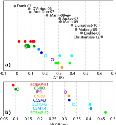
Fig. 6. (a) Temperature change in the MCA–LIA transition for
NH simulations and reconstructions in Tables 1 and 4, respectively. Solid (hollow) dots depict simulations including (excluding) vol-canic forcing. (b) TEF change corresponding to the forcing applied to the simulations in (a). In the case of models for which simulations are available with and without volcanic forcing, the change in the sum of anthropogenic and solar forcing (see Fig. 1f) is shown with a hollow dot and the TEF (see Fig. 1g) change is indicated with a full dot. In the case of the simulation with the ECHO-G model showing warmer medieval temperatures (Gonz´alez-Rouco et al., 2003), the version corrected by Osborn et al. (2006) is considered instead. In the cases where there is overlap of dots, these have been slightly moved in the vertical direction for visibility.
an important contributor to the energy balance in the MCA-to-LIA transition (e.g. Crowley, 2000; Bauer et al., 2003; Goosse et al., 2005). However, other factors like land cover changes (Goosse et al., 2006a) or internal variability (Goosse et al., 2012a,b) may have also been relevant, particularly at regional scales.
in Mann et al. (2009), facilitating the comparison with previ-ous works. Additionally, such a definition of the MCA (950– 1250 AD) is convenient here since it spans a period long enough to include the respective medieval maxima of the simulations, their associated forcings and the reconstructions (see Sect. 5.1).
Figure 6 displays positive MCA–LIA differences in forc-ing as well as in simulated and reconstructed temperature changes, except for the reconstruction of Frank et al. (2007). This curve peaks in the late 10th and early 11th century and reports steeply cooling temperatures until the beginning of the 14th century, similarly to D’Arrigo et al. (2006) and Christiansen and Ljungqvist (2012a). The balance of these temperature anomalies in the Frank et al. (2007) reconstruc-tion during the MCA interval is negative. The range of tem-perature changes in the reconstructions is somewhat larger than in the models, which makes it difficult to determine which combination of solar and volcanic forcing is more re-alistic. Changes in forcing are clearly grouped into the STSI and ssTSI division established in Sect. 3. The temperature changes are also organized accordingly, suggesting that so-lar forcing is a major player in the model simulations of the MCA–LIA transition. Nevertheless, the ssTSI simula-tions of CSIRO and EC5MP-E1, with the largest temperature changes, present values close to those of some STSI experi-ments showing the lowest temperature change (CSM1.4 and CCSM3).
The effect of volcanic forcing is only evident in the ECHO-G simulations for which including volcanic forcing enhances both the MCA–LIA forcing change and the simu-lated response. For the CSIRO model, inclusion of volcanic forcing has no effect on the forcing and temperature changes. These results do, however, depend on the periods used to de-fine the MCA and LIA (not shown). Interestingly, members of an ensemble sharing the same external forcings (CSIRO, ECHO-G, EC5MP) show a spread of temperature changes due to internal variability. This spread may be larger than the temperature difference due to the inclusion of volcanic forcing (ECHO-G and CSIRO) or than the differences be-tween simulations within the ssTSI and STSI groups. For in-stance, intra-model variability in the EC5MP and the CSIRO ensembles is larger than inter-model differences between the CSM1.4, CCSM3, ECHO-G or IPSL simulations. Therefore, this suggests that internal variability could have had major impacts on the temperature response at hemispheric scales.
Additional insights on the relative roles of internal ver-sus forced variability can be gained by considering the spa-tial distribution of simulated temperature changes during the MCA–LIA transition. Many studies (e.g. Seager et al., 2007; Mann et al., 2009; Graham et al., 2011) suggest that dur-ing this period there was a pattern of coordinated temper-ature and hydrological anomalies, evidencing an increased zonal gradient in the tropical Pacific produced by anoma-lous cooling in the eastern Pacific and anomaanoma-lous warmth in the western Pacific and Indian Ocean. Additionally, a broad
expansion of the Hadley cell with an associated northward shift of the zonal circulation might have led to a more pos-itive North Atlantic Oscillation (NAO) like signature (Gra-ham et al., 2011; Trouet et al., 2009, 2012). The relative importance of forcing and internal variability in producing this coordinated pattern of anomalies is not clear. Mann et al. (2009) showed a reconstructed pattern of MCA–LIA tem-perature change indicating enhanced and pervasive cooling in the eastern equatorial Pacific cold tongue region, often re-ferred to as a La Ni˜na-like background state, as well as pos-itive anomalies dominating at mid- and high latitudes of the NH. Mann et al. (2009) also showed that the negative anoma-lies in the eastern equatorial area were not reproduced by forced simulations with the GISS-ER and CSM1.4 models. Extratropical warmth was also reported by Ljungqvist et al. (2012) and was found to be consistent with results of assim-ilation experiments (Goosse et al., 2012a,b) in response to a weak solar forcing and a transition to a more positive Arctic Oscillation state. AOGCM experiments without data assim-ilation, however, do not seem to support an enhanced zonal circulation during medieval times (Lehner et al., 2012; Yiou et al., 2012).
Figure 7 shows the MCA–LIA annual temperature differ-ences (hatched areas indicate non-significance for an α < 0.05 level) in the forced simulations from each of the models considered herein except for the HadCM3 run, which is not included due to the limited time span of this simulation (see Table 2). The reconstructed MCA–LIA temperature pattern from the Mann et al. (2009) multiproxy climate field recon-struction is also shown in Fig. 7 for comparison. The value of the spatial correlation coefficient between each simulated and the reconstructed MCA–LIA pattern is shown at the bot-tom of simulated panels in Fig. 7. For the ssTSI models a selection of the ensemble members is made considering ei-ther the runs with a more complete configuration of external forcings (i.e. the three members including volcanoes), in the case of the CSIRO, or the three runs that represent the most different spatial patterns, in the case of the EC5MP-E1 en-semble. For the EC5MP-E2 all the members of the ensemble are shown. For the ECHO-G, the run with a too-warm MCA (Osborn et al., 2006) is excluded.
Fig. 7. MCA–LIA (950–1250 AD minus 1400–1700 AD) annual mean temperature difference in forced simulations produced by the
AOGCMs with millennium-long simulations in Table 1 and in the multiproxy climate field reconstruction from Mann et al. (2009). The spatial correlation (r) between each simulated MCA–LIA pattern and the reconstructed field is shown at the bottom right of each panel. For the simulations starting in 1000 AD (CCSM3, ECHO-G, IPSL, CNRM), the period 1000 to 1250 was selected instead to define the MCA. Hatched areas indicate non-significant differences according to a two-sided t-test (α <0.05).
multiple regional features that are dependent on the model considered, i.e. cooling in the North Pacific (ECHO-G-1), in the North Atlantic (CCSM3 and ECHO-G-2) or in North-ern Asia (CNRM). This causes the lowest inter-model spa-tial correlation values, both in the STSI (e.g.r= −0.09 be-tween CNRM and CSM1.4) and in the ssTSI group (e.g.r= −0.14 between members of EC5MP-E1 and CSIRO). Many
and CSIRO members. These differences within an ensem-ble lead to intra-model spatial correlation values that range between 0.21 and 0.52 for the EC5MP-E1, between 0.05 and 0.52 for the CSIRO, and between 0.60 and 0.81 for the EC5MP-E2 subensemble. Among the different subensem-bles, EC5MP-E1 and CSIRO simulate more regional/large-scale widespread cooling, a sign of the lower weight of TSI changes that allows for internal variability to become more prominent. This fact can b