Optimising a weighing protocol for sheep

(1)

Lincoln University Digital Dissertation

Copyright

Statement

The

digital

copy

of

this

dissertation

is

protected

by

the

Copyright

Act

1994

(New

Zealand).

This

dissertation

may

be

consulted

by

you,

provided

you

comply

with

the

provisions

of

the

Act

and

the

following

conditions

of

use:



_you

_will

_use

_the

_copy

_only

_for

_the

_purposes

_of

_research

_or

_private

_study



you

will

recognise

the

author's

right

to

be

identified

as

the

author

of

the

dissertation

and

due

acknowledgement

will

be

made

to

the

author

where

appropriate

(2)

OPTIMISING A WEIGHING PROTOCOL FOR SHEEP

__________________________________

A dissertation submitted in partial fulfilment of the requirements for the Degree

of

Bachelor of Agricultural Science (Honours)

at

Lincoln University by

R. F.Wilson

_______________________________

Lincoln University

(3)

ii

Abstract of a dissertation submitted in partial fulfilment of the requirement

for the Degree of Bachelor of Agricultural Science (Honours)

Optimising a Weighing protocol for sheep

By

R.F. Wilson

A series of experiments designed to investigate live weight error and analyse the effect fasting and multiple weighing has on live weight measurements were carried out. In the first experiment 24

mixed aged ewes were fasted during a 24 hour period with live weight measurements taken at 0,

2, 4, 6, 8, 10, 12 and 24 hours fasted, with three measurements taken at each time point. At the

conclusion of weighing all animals were slaughtered and their gutfill was weighed to enable

calculation of their true (digesta-free) weight. In the second experiment 100 Coopworth ewes were

weighed as described above on two separate occasions in May and July. On all occasion animals were individually identifiable with either visual ear tags or electronic identification tags (EID).

In experiment one live weight of ewes at the start of fasting ranged from 34.4 – 79.6 kg with a mean

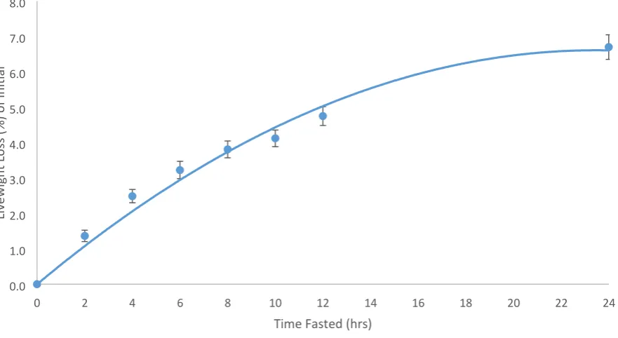
live weight of 61.3 kg. The mean live weight loss displayed a curvilinear response peaking at 4.1 ±

0.23 kg or 6.7% ± 0.348 at 24h fasting, with a significant effect of time. The regression equations y

= -0.0073x2_{+ 0.3445x for absolute live weight loss and y=-0.012x}2_{+0.5636x for proportional live}

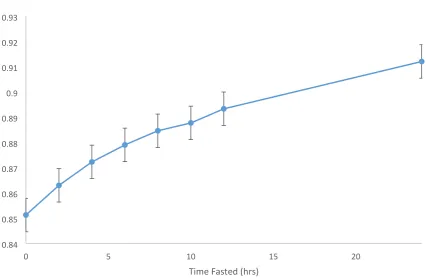
weight loss both explained 98% of the variation. The proportion of true live weight relative to measured live weight over 24 hours fasted increased from 0.85 ± 0.006 to 0.91± 0.004. Despite

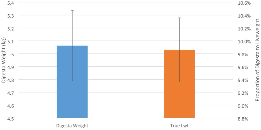
being fasted for 24h the animals were only able to reach 91% of their true live weight as final digesta

ranged from 2.5-7.3 kg with an average of 5.06 ± 0.27 kg. Therefore it was determined that attaining

a reliable estimation of an animal’s true body weight is unachievable when fasting them for 24 hours.

In experiment two, the live weight of 100 ewes was measured during a 24 hours fasting period with

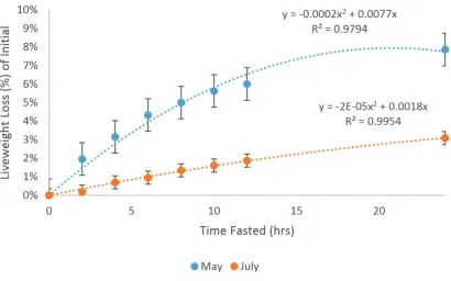
measurements taken at 0, 2, 4, 6, 8, 10, 12 and 24 hours in May which was repeated again in July. The live weight loss peaked at 7.87% in May which was considerably greater than the maximum live

weight loss of 3.09% seen in the July experiment. The difference was likely due to a difference in

(4)

iii animals. The relationship between live weight loss (kg) and (%) ranking at 24 hours fasted and the live weight loss (kg) and (%) at fasting times 2, 4, 6, 8, 10, 12 for experiment 2 (May and July) was

analysed. The strongest relationships were seen at 12 hours fasted: y=0.9878x (R2 _{=0.8976); for}

May, y=0.9567x (R2 _{=0.6623) for July when expressed in kg. As a proportion of weight loss the}

greatest relationship was seen at 10 hours y=0.716x (R2 _{=0.8578) and y=0.8895x (R}2 _{=0.8895) for}

May and July respectively. Probit analysis to fit 95% of their 24hr weight showed no significant

difference was seen between the liveweight range from 0, 2 and 4 hours fasted; 4, 6, 8 hours fasted and 6, 8, 10, 12 hours fasted. In order to analyse the effect of multiple weighing a probit analysis

to determine the range in weight which 95% of average the of three weights would fall indicated

the only significant difference was at 10hrs fasted between one weight and the average of two

weights.

In summary, live weight is a fundamental measurement which is used to monitor the production in

the sheep industry. However live weight is only an estimate of an animal’s true live weight which is unable to be reliably determined even following 24h fasting due to the variation in digesta

weights. Relative to their 24h fasted live weights, fasting improved the accuracy and precision of

the live weight estimate with little advantage observed when animals were fasting for periods

greater than 8h. The method of multiple weighing had minimal effect on improving accuracy

(5)

iv

LIST OF TABLES

Table 2.2.1: Accuracy of scales tested by Kondinin Group ... 5

Table 2.3.1: Mean percentage loss in live weight relative to time off feed off various feeds ... 8

Table 2.4.1: Variation in live weight ± s.e.m (kg) from the best estimate of the true live weight of an animal, derived as the mean of three weighings, required to include a given percentage of the population for when the of the population for when the first recorded weight alone or the mean of the first two weights for animals fasted 0, 24 hours. ... 9

Table 2.5.1: Mean Live weight over each killing (kg) ... 11

Table 2.5.2: Live weight changes (kg) during different periods of the season of Carcass fat weight, internal fat weight and carcass weight. ... 12

Table 2.8.1: Proportional Changes between carcass fat weight, internal fat weight and carcass muscle weight between scanning events ... 15

Table 2.9.1: The association between BC and Ewe Output (Total Lamb Weaned kg) ... 17

Table 2.11.1: Change in liveweight to BCS (SCARM) ... 18

Table 4.5.1: 24 Hour Ranking Data: Live weight Loss (kg) of 24hr ... 45

Table 4.5.2: Live weight Loss (%) of 24hr ... 45

Table 4.5.3: 24 Hour Ranking Data ... 45

Table 4.6.1: The range of live weight (kg) (± s.e.m) within 95% of 24hr weight (kg) for average of 3 weights with time fasted 2, 4, 6, 8, 10 and 12 hours for experiment two May and July. ... 46

Table 4.7.1: R2_{Values for Best Fit Regression for the estimated live weight vs. true liveweight over} multiple weighing: one weight, average of 2 and 3 weights for the 24 ewe experiment. ... 47

(9)

viii

LIST OF FIGURES

Figure 2.1: Histogram showing the results of repeated weighing of one pig using the averaging method ... 5

Figure 2.2: The results of repeated weighing averaging simulating worst case scenario ... 6

Figure 2.3: Percentage of live weight loss from initial live weight of weaned and unweaned lambs

during fasting. Source: (Hughes, 1976) ... 10

Figure 2.4: Body Condition Score Guide ... 13 Figure 2.5: Change in Live weight relative to condition score: Coopworth (2011-2012) & Rosebank

... 19

Figure 4.1: Mean of three repeated measurements of live weight (kg ± s.e.m) relative to time fasting

time from feed and water (h) for 24 ewes. The line of best fit represented the logarithmic equation

y=0.0062x2-0.3074x+61.074 (R2_{=0.988). ... 25} Figure 4.2: The Mean live weight loss of initial live weight in absolute terms (kg ± s.e.m) relative to

time fasting time from feed and water (h) for experiment one (24 ewes). The line of best fit

represented the logarithmic equation y=-0.0073x2+0.3445x (R2_{=0.9845). ... 26}

Figure 4.3: The Mean live weight loss as a percentage of initial live weight (% ± s.e.m) relative to

time fasting time from feed and water (h) for experiment one (24 ewes). The line of best fit

represented the logarithmic equation y=-0.012x2+0.5636x (R2_{= 0.9823). ... 26}

Figure 4.4: The Proportion of Measured Live weight is of True Live weight (proportion ± s.e.m)

relative to time fasting time from feed and water (h) for 24 ewes. ... 27

Figure 4.5: Mean final digesta weight at 24h fasted (kg ± s.e.m) along with the proportion of digesta

to true live weight (proportion ± s.e.) ... 28 Figure 4.6: The Mean live weight loss as a percentage of initial live weight (% ± s.e.m) relative to

time fasting time from feed and water (h) for 100 ewes in experiment two. The line of best fit for

the May Experiment represented the logarithmic equation y=0.0002x2_{+0.0077x (R}2_{=0.9794) and}

the line of best fit for the July Experiment represented the logarithmic equation y=-2E-05x2_+0.0018x

(R2_{=0.9954). ... 29}

Figure 4.7: The Coefficient of variation for the live weight loss (kg) and the live weight loss as a percentage of initial live weight for experiment one... 30

Figure 4.8: The overall coefficient of variation (± s.e.m) of the proportion of measured live weight is

of true live weight relative to time fasting time from feed and water (hrs) for 24 ewes. ... 31

Figure 4.9: The Coefficient of variation for the live weight loss as a percentage of initial live weight

(10)

ix Figure 4.10: Rank Comparison of initial live weight less the true live weight ranking with ranking of live weight loss (kg) for fasting times 2, 4, 6, 8, 10, 12, 24 hours for experiment one (24 ewes) ... 34

Figure 4.11: 24hr Live weight Loss (kg) comparison with live weight loss (kg) for fasting times 2, 4,

6, ... 35

Figure 4.12: 24hr Live weight Loss (kg) comparison with live weight loss (kg) for fasting times 2, 4,

6, 8, 10, 12, 24 hours for experiment two (May). ... 37

Figure 4.13: 24hr Live weight Loss (kg) comparison with live weight loss (kg) for fasting times 2, 4, 6, 8, 10, 12, 24 hours for experiment two (July). ... 38

Figure 4.14: 24 hours live weight loss proportion of initial live weight (%) comparison with live

weight loss proportion of initial live weight (%) for fasting times 2,4,6,8,10,12 24 hours for

experiment 1. ... 39

Figure 4.15: 24hr Live weight Loss proportion of initial live weight (%) comparison with live weight loss proportion of initial live weight (%) for fasting times 2, 4, 6, 8, 10, 12, 24 hours for experiment

two (May). ... 40

Figure 4.16: 24hr Live weight Loss proportion of initial live weight (%) comparison with live weight

loss proportion of initial live weight (%) for fasting times 2, 4, 6, 8, 10, 12, 24 hours for experiment

two (July). ... 41 Figure 4.17: Rank Comparison of 24 hour live weight loss (kg) ranking against ranking of live weight

loss for fasting times 2, 4, 6, 8, 10, 12, 24 hours for experiment one (24 ewes). ... 42

Figure 4.18: Rank Comparison of 24 hour live weight loss (kg) ranking against ranking of live weight

loss for fasting times 2, 4, 6, 8, 10, 12, 24 hours for the 100 ewe May experiment. ... 43

Figure 4.19: Rank Comparison of 24 hour live weight loss (kg) ranking against ranking of live weight loss for fasting times 2, 4, 6, 8, 10, 12, 24 hours for the 100 ewe July experiment. ... 44

Figure 4.20: The range of live weight (kg) (± s.e.m) within 95% of the average of three live weight

mean 24hr weight (kg) for average of 3 weights with time fasted 2, 4, 6, 8, 10 and 12 hours for the

(11)

x

List of Plates

(12)

1

1 General introduction

1.1 Introduction

Live weight measurements are fundamental for livestock production and breeding systems, as well

as experimental research (Allden, 1970; Lawrence, Fowler, & Ebrary, 2002). The live weight of a

living organism includes factors such as carcass composition of bone, muscle, fat, gut-fill content within the alimentary trait, internal organs, head content, pelt and wool. Recording and storing live

weight data has become an easy, cost effective measurement with the use of technologies such as

automated weighing setups, RFID and software systems. In practice and in experimental work it is

often important to determine the growth rate of an animal. Monitoring live weight records are

important for accurately meeting market specifications, reproduction performance, determining

grazing management and for animal health and welfare issues (Sheep CRC, 2012). However, estimating growth rates of animals through weighing live weight is dependent upon the validity of

live weight data (Hughes, 1976). Weighing an animal is an estimation of the animal’s live weight

measurement and therefore will always include some degree of error. According to Hughes (1976)

and Lawrence et al. (2002), there are three factors contributing to the validity of weighing animals; the precision of the weighing machine, human error and the accuracy in apparent changes of live

weight representing true changes in the animal’s actual weight. It appears the third factor has the

greatest influence on accuracy of measurements, as human error can be eliminated by the use of

automated weighing platforms and data storage, and the error associated with weighing machines

is constant and often minimal.

The change in live weight can be the result of increases and decreases in adipose and muscular

tissue although variation is also expected between animals and particularly between different feed

types and periods of weighing due to diurnal variation in gut fill. As expected, live weight fluctuates during the season depending on given nutritional stresses and environmental conditions. It appears

such changes in the body throughout the season are not truly aligned with live weight change with

subsequent changes in live weight over a season from premating, lambing, mid-lactation and

weaning not exactly reflecting the change in total live weight (Field, Suttle et al., 1968; Lambe et

al., 2003). Further, energy changes can be assessed through either Body Condition Scoring (BSC) or

Computed Tomography (CT) scanning and may not truly align with changes in live weight. It is suggested that some of this misalignment is due to weighing error and therefore defining an optimal

weighing protocol is important. Sources of error may include the weight measurement itself, which

(13)

2 the rumen contents, which may be expected to contribute up to 17% of the measured weight, and may be determined by fasting. This review will focus on the variation and error associated with live

weight measurements, the impact of fasting and multiple weighing, the seasonal changes in live

weight, the relationship between live weight and body composition and the uses of live weight

measurements in practice.

(14)

3

2 Review of the Literature

2.1 Measuring Live weight

The process of measuring live weight has made considerable developments from a manual system

to a highly efficient automated set-up, due to the use of Radio Frequency Identification (RFID) and

automated equipment. Historically, measuring live weight involved reading identification tags and weights from the scale and recording on paper, while manually operating weight crates and gates.

The excessive data handling involved in manually recording live weight has a greater risk of error

and inaccuracy of information. Advances in technology have led to the use of electronic, automated

systems, with minimal opportunity for translation errors.

The RFID system consists of 3 main components; an electronic tag, which is located on the animal

for identification; the RFID tag reader, capable of reading and writing data to a transponder, which can be fixed or handheld; and the data processing subsystem, which uses the data in some useful

manner (Engels, Scharfeld, & Sarma, 2007). As the animal approaches the weighing platform, the

RFID reader sends a radio signal which excites the electronic transponder located in the animal. This

then transmits a unique 16 digit number back to the reader. The electronic tag identifies the animal

which is picked up by the fixed EID reader panels via cables or bluetooth. The load bars are located

under the platform which send measurement signals to the weigh head unit from the electrical resistance placed on the bars by the animal (Nugent, 2005). This information is recorded and can

be transferred to a computer and entered into farm management software (Development., 2014).

Another variation on the weighing system explained above is manually operating the weight grate and entering each animal identification code into the head unit.

The resistance on the load bars located under the weight grate are used to determine an estimation

of an animal’s weight. There are two methods by which electronic weigh scales operate; a

measurement will be taken when it is detected that animal movement is stabilised; or a measurement is given by using a statistical process from which several readings taken by the

processor are averaged over a period of time (Smith & Turner, 1974). The first method relies on a

stable period, which is often hard to achieve with animal movement fluctuations resulting in

inaccuracies (Smith & Turner, 1974). The second method has proven to be more useful in practice,

(15)

4

2.2 Measurement Error

2.2.1 Human Error

Historically, weighing animals and recording live weight measurements was a manual and labour

intensive task. In a manual setup individual tag numbers are read and recorded with the resulting

live weight measurement. The data may then be further handled to make use of. This manual

system relies heavily on the operator’s ability to accurately record data while manually operating weighing equipment. The potential for human error has been reduced with the use of various

technologies available to measure live weight. The automated electronic weighing system, with the

use of RFID tags and computer software to clearly display data is probably the most effective system

that reduces the chance of human error.

2.2.2 Scale Error

There are two methods by which weigh scales interpret an animal’s live weight on the load bars

(Nugent, 2005). Either a single weight is recorded during a stable period, when the animal has

reduced movement, or a statistical process is used where the processor takes several readings over

a short time period and averages them. It is difficult in practice to have long durations of stable periods and minimal movement, so the second method is often used (Smith & Turner, 1974).

The variation associated with weighing scales is expected to be very minimal, as technology has

advanced. It is suggested that accuracies of ±1% of actual weight, or 0.91 kg for sheep is sufficient (Smith & Turner, 1974). Aiming for an accuracy of ±1% is desirable, given a 65 kg ewe variation can expect to fluctuate ±0.65 kg. There is little research on specific weighing equipment accuracy for sheep, however, in most cases the same scale will be used for all animals in a weighing session,

therefore the variation will be the same across all stock. A recent Australian study revealed that the variation of five commercial scales ranged from ±1.9 kg to 2.8 kg for ewe body weight, see Table 2.1 (Nugent, 2005). The results from the Australian trial showed scale variation was greater than

(16)

5

Table 2.2.1: Accuracy of scales tested by Kondinin Group

Scale type Average Weight (kg)

Correlation (Accuracy)

Precision 95% Confidence Interval

Iconix FX41 45.9 0.986 ± 1.9

Prattley draft crate 45.1 0.954 ± 2.2

Ruddweigh 600 45.7 0.981 ± 1.9

Thunderbird Ultrascale 44.9 0.957 ± 2.8

Tru-Test XR3000 44.9 0.38 ± 2.2

Source (Nugent, 2005)

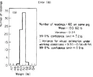
Another study in relation to pig scales reported 99.8% confidence limit of ± 2lb of the correct value using the averaging method, see Figure 2.1 (Smith & Turner, 1974). In addition a worst case scenario

Figure 2.2 was simulated using a 152.5lb man to violently shake the weighing crate. Weight variation

was calculated to be within ±2lb. Both live weight experiments had acceptable variations, around 1% proportional to body weight.

(17)

6

Figure 2.2: The results of repeated weighing averaging simulating worst case scenario

There is little research into scale error for commercial sheep scales including automatic weighing. The precision of a live weight is known as how close any weight is to the true live weight of an animal

(Nugent, 2005). However, a live weight measurement is only an estimate as it is impossible to attain

a true live weight reading on an animal at any given time. The accuracy of an estimated live weight

can be shown by the variation in a repeatable estimate. It is acknowledged that there will always be

a scales error which causes variation and it has been suggested that there is little advantage in obtaining fine precision; (Smith & Turner, 1974); (Hughes, 1976). Although attaining a greater

accuracy may be useful in scientific experiments or when animals are weighed on an individual

bases.

2.3 Live weight Error

2.3.1 Gutfill Variation

The digestive tract can make up a high proportion of an animal’s mass, with up to 17% of total live weight accounted for in the contents of the rumen and reticulum (Lawrence et al., 2002). The

amount of feed and water within the digestive tract is dependent on the time since the animal was

fed and the rate of food passage (Hughes, 1976). It should be considered that weighing live animals

will include an amount of gutfill, which will vary between animals, time of day measured, time off feed and previous feed type.

2.3.2 Diurnal Variation

The pattern of grazing events will dictate how much feed an animal has at any given point in time

and therefore will influence the live weight and live weight changes throughout the day. Ruminants

generally have three to five grazing events daily, with greatest intake periods to be in the early morning and late afternoon (Gregorini, Gunter, Beck, Soder, & Tamminga, 2008). Penning, Rook et

al. (1991) reported ewe grazing patterns with 70-99% of grazing occurring during daylight hours and

25-48% during the 4 hours prior to sunset. In comparison, cattle have been reported to have around

(18)

7

time at which the animals are weighed has a large effect on the amount of gut fill within an animal. Animals weighed at the start of the day will have a limited time grazing and therefore may have a

reduced gut fill status compared with animals weighed mid-afternoon. Grazing patterns vary

between animals depending on herbage quality, type of herbage and the environment. The timing

of grazing events in relation to the timing of weighing animals can have a significant impact on the

animal’s estimated live weight. Herbage DM % increased during a 12 hour period from 15-24% grass

and 12-18% clover. Starch content also increased 3-4.1% and 3.6-8.7%, for grass and clover respectively (Orr, Penning, Harvey, & Champion, 1997). In respect to grazing behaviour, animals are

more inclined to gorge themselves on lower dry matter and lower starch pastures. According to

Hamilton (1995), the greatest diurnal variation in estimated live weight was observed between

11am-1pm and the lowest variation reported at 9am and 4pm, with sunrise at 6am. In agreement,

Hughes (1976) suggested weights taken at the middle of the day from a grazing period on a limited area were least variable. It is also recommended to muster animals before grazing to minimise gutfill

error (Hughes, 1976). Diurnal variation should be considered when designing a weighing protocol,

however a system should be adopted that is practical to the situation.

2.3.3 Feed Type Factors

The feed type along with diurnal factors have a major impact on gutfill. Sheep on lower quality, high

fibrous feed have a low passage rate, which may lead to a reduced intake and gutfill. The greater the

Neutral Detergent Fibre (NDF) content, the slower the passage rate. Conversely, sheep on high

quality feed may have higher intakes, greater gutfill and passage rates. Therefore it can be assumed

that true body weight is often overestimated for animals on high quality feed, in comparison with animals on lower quality feed. Table 2.3.1 shows differences between feeds with the average

percentage of live weight lost greater in lupins and lucerne, in comparison with pasture in lambs.

However, it should be noted that there was large variation within data and between different stock

(19)

8

Table 2.3.1: Mean percentage loss in live weight relative to time off feed off various feeds

Time off Feed (hr)

2 3 4 5 6 8 10 12

Pasture -Lambs 1.18 1.54 1.41 2.07 3.05 2.52 2.75 3.22 4 4.31 3.07 6.21 6.21 4.83 4.71 6.36 8.96 Lupins -Lambs Lucerene -Lambs Pasture -Hogget Pasture - 70d pregnant

Source: (Greer, Logan, & Bywater, 2013)

Feed type factors are largely dependent on the environment and how the stock are managed. Sheep

stocked at a higher stocking rate will have a greater grazing pressure and therefore are likely to have

a lower average gutfill and digestibility. It is important to recognise feed quality and quantity factors between flocks prior to weighing, so that such factors are accounted for (Hughes, 1976).

2.4 Reducing Live weight Error

2.4.1 Multiple Weighing

In order to take a reliable live weight measurement of an experimental animal, Bean (1946) believes

it is necessary to take more than one measurement. Taking multiple weight measurements of an

animal over a period of time reduces the reliance on a single measurement and exposure to the

associated error. Lush et al, (1928) recommended to weigh cattle over three consecutive days to remove inaccuracies associated with live weight measurements. This practice was recommended as

a standard procedure for cattle in 1931 by a committee of the American Society of Animal

Production (1932) as cited in (Patterson, 1947). In the original cattle study (Lush & Black, 1927) it

was found the error of a three-day weight is only 57% that of a one-day weight. It is thought that

the improved accuracy is particularly important when analysing the change of live weight on an individual animal bases (Hughes, 1976). However, the theory that three-day weights are more

accurate than one-day weights has been challenged (Baker, Phillips, & Black, 1947); (H. W. Bean,

1946); (H. Bean, 1948). H. W. Bean (1946) found in swine, an increase in error with the use of a

(20)

9

difference was not significant. In agreement, Baker et al. (1947) showed no significant difference between the 3-day average weight of 424.6 pounds and the one day weight of 425.9 pounds on 178

heifer and steer calves. In the 420-439 pound group, the error increased throughout the trial, first

day weights (428.5 ± 1.19); second day (427.6 ± 1.75); third day (427.7 ± 2.35) with the threeday average (427.7 ±1.66). Bean (1946) also concluded, using swine, that there was no increase in accuracy with using three-day weight averages versus one single measurement. Bean (1946) showed

variation increased with multiple weighings with the 27-38 pound group weighing 31.47 ±.40 pounds on the first-day weights; second day 31.66 ±.45; third day 32.03 ±.43; three day averages 31.67 ± .42. Bean (1948) suggested that the weather conditions and physical conditions animals are under

prior to weighing determine the difference between one day and three day weighing’s averages. In

the trial of Bean (1946), the lambs were not accustomed to being handled or the weighing process

as they were brought in from the Western ranges just before the trial. It is expected animals will become familiar with the weighing environment with repeated weighing. However, it is accepted

that weighing animals over consecutive days is impractical, especially in a pasture grazing system. A

study by Galwey, Logan, and Greer (2013), quantified the variability of a live weight estimate over

24 hours fasting and with multiple weighing, shown in Error! Reference source not found.. The study

evealed that the average of two weights improved the accuracy of weight compared with the use of a single weight, however this is to be expected as the comparison of the best estimate was made to

the average of three weights. At 0 hours fasted 99% of data from the first live weight measurement

was within 0.69±0.16 kg of the best estimate and the average of the first two weights was within

0.31±0.09 kg of the best estimate, this was reduced to 0.43 ±0.02 and 0.22±0.06 kg after 24 hours

fasted respectively. The minimal improvement in accuracy of weights made by weighing multiple times, if any, may not be worth the effort involved in labour and handling stock multiple times.

Table 2.4.1: Variation in live weight ± s.e.m (kg) from the best estimate of the true live weight of an animal, derived as the mean of three weighings, required to include a given percentage of the population for when the of the population for when the first recorded weight alone or the mean of the first two weights for animals fasted 0, 24 hours.

Proportion of 0 hours fasted 24 hours fasted

samples (%)

1st Weight 1st and 2nd Weight

50 85 95 99

0.08 ± 0.07 0.35 ± 0.10 0.52 ± 0.12 0.69 ± 0.16

0.01 ± 0.10 0.14 ± 0.05 0.22 ± 0.05 0.31 ± 0.09

0.08 ± 0.01 0.24 ± 0.01 0.33 ± 0.01 0.43 ± 0.02

0.04 ± 0.02 0.12 ± 0.02 0.16 ± 0.03 0.22 ± 0.06

(21)

10

2.4.2 Fasting

Fasting is a common practice in the sheep industry recommended before shearing, transport and

pregnancy scanning. Fasting results in a curvilinear loss in live weight, with gutfill the main

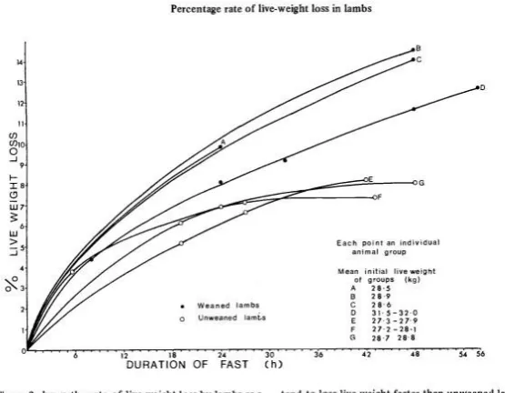
component of live-weight loss during the first 24 hours fasted, Figure 2.3. Thompson, O'Halloran,

McNeill, Jackson-Hope, and May (1987) also demonstrated this curvature response in lambs with

0.82% lost in the first 0-3hours; 0.47% in 3-6 hours; 0.39% from hours 9-12 and 0.25% between 2448

hours. There is little research conducted in the first 24 hours to compare percentage loss particularly in older stock. Live weight losses observed in fasting lambs equated to 5.25% of initial live weight

during the first 24 hours, with only 2.48% during the following 24 hours (Warriss, Brown, Bevis,

Kestin, & Young, 1987). However, it should be noted that water was not restricted during fasting,

possibly explaining the low values of live weight loss. The result of fasting within the first 24 hours is largely due to losses in gutfill, and therefore the diurnal pattern becomes a major factor in the

amount of live weight loss. Kirton, Quartermain, Uljee, Carter, and Pickering (1968) reported in

lambs a 33% reduction in the weight of the stomach contents in the first 24 hours of fasting,

confirming the loss is largely due to gutfill. Therefore by reducing gut fill, the animal is likely to be

closer to their ‘true’ live weight, which in turn may be expected to reduce live weight measurement

error.

Figure 2.3: Percentage of live weight loss from initial live weight of weaned and unweaned lambs during fasting. Source: (Hughes, 1976)

(22)

11

Fasting beyond 24 hours results in subsequent tissue loss and is much slower, which explains the tapering off to the curvature response. Previous research has showed live weight losses range from

3.5-15% of an animal’s initial live weight prior to 24 hours fasted. In comparison, live weight losses

in lambs were approximately 9% and 12% after 24 and 48 hours (Thompson et al., 1987). Similar

results were found in >24hr fasting trials with Cole (1995) reporting a 9.9% loss of body weight, of

which 80% was body water and 55.9% of the total weight loss was accounted for with stomach and

gastrointestinal trait contents and tissue. The differences between experiments is likely due to the different gutfill at the start of fasting.

2.5 Seasonal Changes in Live weight

As expected, live weight fluctuates throughout the season. This can be influenced by the environment and the energy demands placed on the animal at any given time. Table 2.5.1 indicates

the difference in Blackface ewes’ live weight during a given season as reported by Field, Suttle &

Gunn, (1968). Live weight declined from November through to May, during pregnancy and lactation.

However, not all live weight loss was represented by the change in body tissue.

Table 2.5.1: Mean Live weight over each killing (kg)

Source (Field, Suttle, & Gunn, 1968)

Another important factor to consider is the increase in conceptus weight as pregnancy increases.

This indicated that there is possibly some error associated with weighing the animals or the change

in tissue that is not fully represented by live weight changes. Similarly, NR Lambe et al. (2003) found

live weight fluctuations during the season in Scottish Blackface ewes, shown in Table 2.5.2 with predicted tissue weight changes in barren ewes An increase in live weight was reported from

midlactation to weaning, weaning to pre-mating across all animals and pre-lambing to mid-lactation

for barren 2 year old ewes (NR Lambe et al., 2003). The greatest loss was found in 2 year old ewes

carrying twin lambs, -3.16 kg at pre-mating to pre-lambing. This may be caused by the low feed

allowance over the winter time period. Table 2.5.2 shows that the amount of live weight loss or gain is varied across different ewe age and number of lambs.

Oct Nov Jan Apr May (L) May (B) July

(23)

12

Table 2.5.2: Live weight changes (kg) during different periods of the season of Carcass fat weight, internal fat weight and carcass weight.

2 Yr Old Ewes 3 Yr Old Ewes

Period in Season 0 Lambs 1 Lamb 2 Lambs 1 Lamb 2 Lamb

Pre-mating to pre-lambing -2.24 -2.99 -3.16 -1.53 -1.91

Pre-lambing to mid lactation 3.47 -2.64 -1.62 -3.65 -0.93

Mid lactation to weaning 4.67 2.95 2.45 3.89 1.70

Weaning to pre-mating 0.79 2.76 2.18 2.92 2.45

Source (NR Lambe et al., 2003)

2.6 Methods of estimating body composition

Estimation of body reserves is an important management tool which can give an idea of the nutritional status of the sheep. Farmers can then feed their animals based on whether they need to

improve their condition, which is particularly important in the lead up to tupping. Body condition

scoring and Computed Tomography are two methods that give an indication of body reserve tissue.

2.6.1 Body Condition Scoring

Body condition scoring (BCS) is a low cost management tool to compare sheep using the tissue

between the last rib and pelvis, ‘loin chop’ region. BCS is a measurement of an animal’s health status

relating to the production ability at one particular point in time. BCS is usually measured on a 1-5

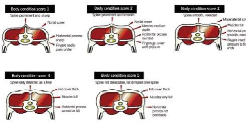
score point scale, depending on the amount of fat tissue present on the last rib, see Figure 2.4: Body

Condition Score Guide (Beef+LambNZ, 2014). An advantage of BCS is that the assessment is independent from frame size, breed, gestation and gutfill. However, in a commercial setting it may

(24)

13

Figure 2.4: Body Condition Score Guide Source (Beef+LambNZ, 2014)

In order to achieve high production, BCS targets can be set at different times of the year, particularly

at tupping. An increase in one BCS at joining can result in an increase in ovulation rate by 0.13 to 0.19. Greater results have been reported of 0.56 of ovulation rate (Gunn and Doney) or 29% increase in

number of lambs (Pollott and Kilkenny) per BCS (SCARM, 1994).

2.6.2 CT Scanner

One method of measuring body composition is with use of a CT (Computed Tomography) scanner, see Plate 2.1. CT scanning was initialling developed for human medicine as a non-invasive way to collect

images and information on body tissue. The scanner works by sending out a series of shortduration,

very narrow, fan-shaped beams of radiation (CREDO., 2000). Detectors rotate a full 360 degree angle

around the animal and scan it. The detectors on the opposite side detect the absorbance of x-rays,

which is dependent on the type and density of the tissue as it passes through the circular cavity (Lincoln

University, 2011). One type of analysis is the Cavalieri, which takes cuts every 50mm with the density averaged out by the distance of each area. However, in most cases the seven reference slices are

accurate enough to estimate muscle and adipose tissue. The body composition is estimated using CT

(25)

14

Plate 2.1: CT scanner

2.7 Change in Tissue

The proportion each adipose tissue site adds to the total carcass weight varies in different breeds of

sheep, due to the final mature weight and the time taken to reach this weight, accounting for some of

the variation described above. The order of tissue development is firstly through bone deposition, then muscular and finally adipose fat. Changes in bone composition as total body composition are very

minimal, often the focus is towards protein and adipose distribution. It is thought that most

hyperplasia in the perennial tissue is complete at the birth of a lamb (Lawrence et al., 2002). After this,

hyperplasia is observed up to 100 days after birth, resulting in an increase of adipocytes in the

subcutaneous and intramuscular deposits. It has been reported that these adipocytes may increase by

2 to 3 fold right up to maturity (Lawrence et al., 2002). The rate the adipose tissue matures at varies between breeds and between different regions i.e. limbs, brisket, thorax, shoulders, loin and rump.

Generally the regions listed above are the last to deposit and the first to lose it in times of feed surplus

and deficit (Frutos, Mantecon, & Giráldez, 1997).

2.8 Season Changes

A major factor in the change in body composition is the stage of season or the physiological state of the

animal. During the season an animal faces different energy demands or different planes of nutrition

(26)

15

throughout the reproduction and lactation season. NR Lambe et al. (2003) found that both carcass and internal fat deposits were depleted during pregnancy and early lactation which were replenished mid

lactation to mating the following period. This may be expected as energy demands one week prior to

lambing for a 60 kg ewe are 16.5 and 20.0 MJME/kg DM for single and twin bearing ewes respectively

(Kenyon & Webby, 2007). Subcutaneous fat was mobilised in preference to inter-muscular fat in Scottish

Blackface ewes, with minimal reduction in muscular deposits (NR Lambe et al., 2003); (Cowan, Robinson, Greenhalgh, & McHattie, 1979). In contrast, Russel et al (1968) as cited in (NR Lambe et al., 2003) found

a reduction in protein and ash content of 20% from pre-mating to the final week of pregnancy. It is

assumed that fat deposits are first used as energy reserves followed by protein losses, which is

dependent on a ewe’s individual body composition. It is suggested that individual ewes hold different

compositions of deposits and therefore in times of nutritional stress different energy stores will be depleted. This could explain the large variation between live weight and body condition score described

above.

The seasonal change in body composition is largely explained by the carcass and internal fat weight, in

barren 2yr old ewes 99% of live weight change was explained by carcass fat. Collectively, carcass and

internal fat weight explained over 50% of live weight change (N. Lambe, Simm, Young, Conington, &

Brotherstone, 2004). From pre-lambing to mid lactation, barren 2 year old ewes have a greater

proportion of carcass muscle weight, which could be explained by the barren ewes having a lower energy demand so any excess net energy can be put towards fat and muscle deposition. The

proportion of different fat and muscle compositions vary largely throughout the season and across

different ages of ewes and number of lambs being carried. However, different body compositions

result in different live weights. The weight of adipose tissue was significantly different, averaging 9.19,

2.28 and 1.19 kg on days 12, 41 and 111 for ewe live weight 60.2, 58.9 and 55.8 kg, respectively. It appears that the ewes lose more adipose tissue than live weight which suggests that the other tissue

was mobilised over lactation and the relationship between adipose tissue and live weight is not

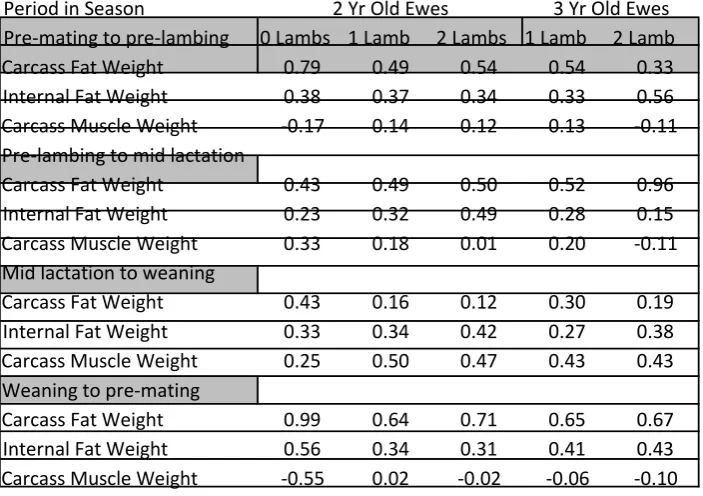
entirely direct and may change throughout the season. In agreement, Table 2.8.1 illustrates the

significant changes in carcass fat deposition between scanning events for barren ewes. In most cases,

a significant result was shown between barren ewes and ewes carrying 1 to 2 lambs, with some differences between 2 and 3 year old ewes. This provides evidence of differences between ewes which

(27)

16

Table 2.8.1: Proportional Changes between carcass fat weight, internal fat weight and carcass muscle weight between scanning events

Period in Season 2 Yr Old Ewes 3 Yr Old Ewes

Pre-mating to pre-lambing 0 Lambs 1 Lamb 2 Lambs 1 Lamb 2 Lamb

Carcass Fat Weight 0.79 0.49 0.54 0.54 0.33

Internal Fat Weight 0.38 0.37 0.34 0.33 0.56

Carcass Muscle Weight -0.17 0.14 0.12 0.13 -0.11

Pre-lambing to mid lactation

Carcass Muscle Weight 0.33 0.18 0.01 0.20 -0.11

Mid lactation to weaning

Carcass Muscle Weight 0.25 0.50 0.47 0.43 0.43

Weaning to pre-mating

Carcass Muscle Weight -0.55 0.02 -0.02 -0.06 -0.10

Source: (NR Lambe et al., 2003)

2.9 Body Composition & Production

The energy demands at particular times of the season result in the mobilisation of tissue. Total energy

reserves are difficult to measure, particularly glycogen and intra-abdominal fat reserves (Kenyon, Maloney, & Blache, 2014). It is expected that a ewe will face body condition changes over the season

shown by fluctuations of BCS. The ability a ewe has to mobilise her energy reserves will in turn

influence the production output or the amount of lamb per ewe. Borg, Notter, and Kott (2009) and

Mathias-Davis, Shackell, Greer, and Everett-Hincks (2011) suggests that ewes which appear to be able

to hold their condition in early gestation and utilise reserves in lactation outperform their peers who cannot. Evidence of this is outlined below in Table 2.9.1, the highest performing ewes were shown to

have a condition score of <3 at weaning, presumably reflecting mobilisation of body reserves. Lamb

growth rates are significantly affected by the change in ewe BCS from pre-lambing BSC to the BCS in

lamb weaned (Mathias-Davis, Shackell, Greer, Bryant, & Everett-Hincks, 2013). These studies indicate

high performing ewes have a greater ability or willingness to mobilise their own energy reserves. This suggests that perhaps farmers should be looking to identify such animals and making the most of this

(28)

17

will undeniably lead to an increase in body mass. Therefore, there is potential to use live weight or change in live weight as an estimation of BSC, providing a more practical method for assessing changes

in body reserves.

Table 2.9.1: The association between BC and Ewe Output (Total Lamb Weaned kg)

Birth Rank

All 1 2 3

<3 48.4 35.4 52.5 60

BCSL 3-3.5 >3.5 48.8 49.7 35.1 34.9 53.3 53.1 61.4 65.2 BCSW <3 3-3.5 >3.5 50.9 48.9 43.8 36.6 35.3 33.8 55.2 52.6 46.8 64.4 62 52.6 BCSL = Body Condition Score Lambing

BCSW = Body Condition Score Weaning

Source (Mathias-Davis et al., 2011)

2.10 Live weight Gain or Loss

Reports have shown after periods of animal feed restriction, there has been an increased rate of fat

deposition (McMeekan 1941, Keys et al 1950, Osborn and Wilson 1960 as cited in (Allden, 1970)). This

suggests that fat tissue more readily deposits than other tissues, when an increase in feed plane is

exerted. However, another study showed weight gain did not really differ from the composition of live weight loss (Meyer and Clawson, 1964 as cited in (Allden, 1970)). There was a small significant result

between control and restricted diet treatments, however no significance was found within the

restricted groups with a range of treatments from 20-84% feed restriction from the control group.

Often animals are restricted from feed during periods where their energy demands outweigh the feed

available or the cost of feed is too high. However, animals are not often effected in the long term as compensatory growth follows periods of nutritional restriction (Ryan, Williams, & Moir, 1993).

The plane of nutrition is another factor that needs to be considered. Ewes which were fed to increase

or decrease by one body condition equated to a 8.72 kg and 8.65 kg in comparison with a static plane

(29)

18

It is obvious that there is large variation between breeds and even within breeds with the amount of live weight change per BCS. This variation has not really yet been explained in research, but it is likely

that changes in gutfill and body composition are major factors.

2.11 Body Condition Score and Live weight Relationship

There is an indisputable relationship between BCS and live weight, as changes in adipose and muscular

tissue will involve an increase in the mass of an animal. The relationship between live weight and BCS

for Merino ewes was 9.2 kg or 0.19 x standard reference weight increase in weight per unit of BCS.

However, there was considerable variation in this relationship even within breed with a range within

of 6.3 – 11.3 kg in merino sheep (Van Burgel et al., 2011). Similarly, Jefferies (1961) as cited in (SCARM, 1994) noted a change of 7 kg in Corriedales and Merinos per unit of BCS. The intercept, or kg of live

weight per body condition score is variable across individual sheep, physiological state and breed.

Table 2.11.1 shows the large variation between breeds, dry and lactating animals. The frame size of

the animal is an important factor to consider, with a greater live weight for 1 unit of BSC in the larger

frame animals. Dorset Down and Polwarth breeds have a greater mature weight resulting in a greater live weight between BCS compared to their smaller frame peers. With that said, considerable variation

in frame size can be expected within breeds as well as between breeds highlighting the difficulty of

providing breed-specific values.

Table 2.11.1: Change in liveweight to BCS (SCARM)

Source (SCARM, 1994)

There is also large variation within breeds between the change in live weight per condition score as

reflected by annual Coopworth and Rosebank data set, shown in Figure 2.5 (Greer et al., 2013). The

equation of best fit for the Coopworth data equated to y = 5.2937x + 4.1776 (R2_{= 0.2) and y =}

. :

Ewes (dry) Change in Lwt (kg) per BCS

Polwarth x SA Merino 6.5

Saxon Merino 5.6

Scottish Blackface 10.6

Ewes (lactating)

Sth Aust Merino 5

Saxon Merino 5.5

Corriedale 11.9

(30)

19

5.0075x + 2.1058 (R2_{= 0.38). The overall change per condition score is 5 kg however, large variation is shown} in Figure 2.5, with a range of 10 kg. In order to use live weight as an indicator of body tissue reserves this

variation needs to be minimised.

Figure 2.5: Change in Live weight relative to condition score: Coopworth (2011-2012) & Rosebank

(2012-2013) Data set

2.12 Use of Live weight Measurements in Industry

Live weight measurements are an easily attainable measurement which are commonly used in the

livestock industry, as outlined below. As outlined above, live weight measurements are exposed to error from a number of sources, all of which may affect both the precision and accuracy of the live

weight estimate. As may be expected, the accuracy and precision of the live weight required is

dependent on the purpose.

2.12.1 Marketing & Selection

Live weight information is collected and goes into the selection process on Sheep Improvement Ltd

(SIL) for the calculation of an animal’s genetic potential for growth targets. Live weight measurements are taken for the growth rates of lambs (g/day) and weaning weight at various ages. Live weight gains,

in particular lamb growth rates, are important to assist in optimising finishing systems and improve

the efficiency of the farming system. Alternatively, the selection of which animals are sent to market

can be made based on live weight and taking into account the expected dressing out percentage.

(31)

20

2.12.2 Determining dose rates

A live weight measurement is needed in order to accurately determine dose rates for drenches and pour on dips. It is recommended to separate mobs into similar weight ranges and drench to the

heaviest weight. The accuracy of the animal’s live weight is important to provide a sufficient dosage

of drench. Ensuring effective drench rates is an important factor in preventing drench resistance. It

can be effective to weigh stock into different lines and drench accordingly to ensure greater efficiency

of drench use.

2.12.3 Monitoring Progress

Monitoring ewe live weight gives an indication of sheep performance on a whole flock or individual

basis. Commonly, a sample of 10% of a flock is weighed to give an indication of flock progress (Edward, 2009). It is important that live weight during tupping period is monitored along with body condition.

Higher weights, along with adequate body condition ewes, have greater ovulation and conception

weights. Ovulation rate was significantly greater between ewes’ conditions 1 ½ and 3 (Gunn, Doney,

& Russel, 1969). As a result, it is expected that greater condition ewes have greater conception rates.

Research conducted by Rutherford, Nicol, and Logan (2003) suggested that the mean ovulation rate was effected by smaller-framed ewes (OR = 0.02616 x jLW + 0.463). However, no relationship was

found between ovulation rate and joining live weight of the larger framed ewes, with maximum

ovulation rate predicted to occur at 67.5 kg joining live weight. It is beneficial for farmers to have a set

target of live weight throughout times of the year, depending on the season and breed of stock. It is

important when setting target live weights that consideration is given to the mature weight of the breed and the availability of feed. It is recommended to aim for at least a 3 out of 5 BCS at tupping

(Rick & Peter Cameron, Southland pg 27 (PGG Wrightsons, 2013), although the optimum live weight

may be dependent on frame size. Measuring change in live weight may reflect change in nutrient

status which is useful from a farm management perspective. Thus the precision of a live weight

estimate becomes more important than accuracy to enable flux in live weight to be assessed. It is suggested that monitoring ewe live weight to identifying the elasticity of ewes could be beneficial for

farmers. As identified in 2.9, body composition and production (Mathias-Davis, 2011) showed ewes

that mobilised their own body reserves over lambing and lactation produced larger lambs, resulting in

a lower BCS. There is potential for live weight measurements to be used to identify high performing

(32)

21

2.13 Summary

The use of live weight measurements to monitor changes in body tissue reserves would be a useful

management tool. However, there is considerable variation within live weight measurements and live

weight changes between BCS. Body condition scoring does give a reliable assessment on energy

reserves, however, it is quite a slow, manual process. Live weight measuring is a quick, automated process which can be assessed in quite a short space of time. However, live weight is only an estimate

of the true live weight of an animal which can only be calculated on slaughter In order to reduce the

variation associated with live weight and the difference between BCS, it is important to uncover where

the variation is coming from. Designing a suitable weighing protocol could reduce some error and help

explain differences between BCS throughout the season.

(33)

22

3 General Methodology

3.1 Experiment 1

The live weights of twenty four mixed-age ewes with a mean initial (non-fasted) live weight of 61.3 ± SEM kg were compared at different times of fasting with their digesta-free weights (true live weight).

The ewes were identified individually with visual ear tags and had been grazing ryegrass white clover

pastures prior to housing. From housing, access to feed or water was withheld for a period of 24h prior to slaughter. This occurred on three separate occasions with ten, six and eight ewes respectively.

At the time of housing and during the 24 hour fasting period, the live weight of each ewe was

repeatedly recorded, as per the weighing protocol described below. Immediately prior to slaughter,

the live weight of each animal was recorded with the weight of digesta contained within the

alimentary tract also recorded post-slaughter, to enable calculation of the true live weight of each individual, as described below.

3.1.1 Weighing protocol

On each occasion, all animals were removed from pasture two hours post-sunrise. Live weight of each

individual was recorded with electronic scales with a sensitivity of 0.2 kg upon removal from pasture

(0hrs fasted) and every two hours thereafter until 12hrs fasting, and again after 24hrs fasting. To obtain a best estimate of live weight at each fasting time, the live weight was recorded three times,

with a maximum of 5 min between each weight recording (run). After 24 hours, fasting animals were

slaughtered. No attempt was made to influence the order in which animals were weighed. For each

fasting time the first recorded live weight was compared with the mean of the three weights to

determine the benefit of multiple weight recordings. The live weight at each fasting time was compared to evaluate the benefit of fasting on reducing the variation in live weight estimates.

3.1.2 Slaughter procedure and true body weight estimates

As described above, after 24 hours fasting animals were slaughtered and the weight of digesta was

measured to enable calculation of the true body weight of each individual. Due to the time taken to slaughter animals (up to two hours), each animal was again repeatedly weighed, as above,

immediately prior to slaughter. For slaughter, animals were stunned with the use of a captive bolt

followed by exsanguination caused by severance of the jugular vein and carotid artery. Immediately

upon death the internal organs including the gastrointestinal tract were ligated and removed. The

(34)

23

removed by running the intestinal material between the thumb and forefinger of the operator and were collected into the same bucket. Care was taken to ensure as much of the digesta was collected

as possible. The digesta contents were then weighed and subtracted from the live weight recorded

immediately prior to slaughter to give the estimate of the true body weight for each individual animal.

Plate 3.1: Emptying gutfill

3.2 Experiment 2

The change in live weight during fasting for a period of 24 hours was recorded in 100 pregnant

mixedage-ewes on two separate occasions (May and July). All ewes had been previously tagged with

individual electronic identification (EID) tags and were shorn 48h prior to the start of measurement to

remove fleece weight as a factor. In the May experiment the ewes were removed from feed, two hours

post-sunrise and deprived of feed and water. Due to poor weather conditions in July the ewes were kept in the yards after shearing and fed baleage prior to the experiment. Live weights were recorded

using an electronic tag reader and automated weighing and drafting unit at the time of removal from

pasture (time 0hrs) and every two hours until 12 hours and again at 24 hours. Fasting occurred in an

identical protocol to that described above, with the an exception being a maximum of 10 minutes

between each triplicate weight recording (run) due to the time taken to weigh all 100 animals. No attempt was made to influence the order in which animals were weighed.

3.3 Statistical Analysis

The statistical software used for analysis was GenStat (version 13, VSN International Limited) and

Minitab 15 (Minitab Inc, version 15, 2006). For Experiment 1, no difference in the profile of live weight

loss, either as absolute weight loss or as a percentage, between the three separate occasions was

(35)

24

fasting trial was considered as one rep, giving three replicates in total (one for Experiment 1 and two for Experiment 2). To determine the benefit of fasting on improving the accuracy of live weight

estimates, regression equations of live weight loss at each fasting time were compared with

digestafree live weight (for Experiment 1) and 24 hour fasted live weight (for Experiments 1 and 2)

using ANOVA. For each rep, the deviation of the first weight recorded from the 24 hour fasted weight

for each fasting time was compared using probit analysis to give the range in weight required to encompass 95% of the population (LD95). The LD95 values for each fasting time were then compared

using ANOVA with 95% least significant differences calculated. Further, the correlations between the

rank of live weight loss between time 0 hours and 2-12 hours (where 1=greatest LW loss) and the rank

of total live weight loss (0hrs less 24hrs) were compared to determine if the relative order of live

weight loss was constant between individuals.

To determine the benefit of multiple weight recordings within time periods, for each rep and for each

fasting time (0 hours to 24 hours) the variation between the first weight recorded or the mean of the

first two weights recorded and the mean of all three recorded weights was calculated. This was compared using probit analysis to calculate the weight variation required to encompass 95% of the

variation (LD95) which was then compared between multiple weighings for each fasting time using

ANOVA with 95% LSD calculated. Further, the regression equations when the y intercept was set to 0

and the regression co-efficient (R2_{) within each fasting time for either the first weight or the mean of}

the first two weights compared with the mean of all three weights were calculated and compared using ANOVA.

4 Results

4.1 Live weight loss relative to fasting time

4.1.1 Experiment 1

Mean live weight of the ewes ± s.e.m. for the average of all three weights recorded at 0h, 2h, 4h, 6h,

8h, 10h, 12h and 24h of fasting is given in Figure 4.1. Live weight of the ewes at the start of fasting

ranged from 34.4 kg to 79.6 kg, with a mean of 61.3 kg.Overall, there was no effect of run (P>0.05)

but there was an effect of time (P<0.001), reflecting a decrease in mean live weight from 61.3 ± 2.53 kg at time 0 to 57.2 ± 2.42 kg at 24h fasting. This reduction was curvilinear, with an equation of best

fit being y = 0.0062x2_{– 0.3074 + 61.074 (R}2_=98.8).

(36)

25

Figure 4.1: Mean of three repeated measurements of live weight (kg ± s.e.m) relative to time fasting time

from feed and water (h) for 24 ewes. The line of best fit represented the logarithmic equation

y=0.0062x2-0.3074x+61.074 (R2_=0.988).

4.1.1.1. Live weight Loss- Experiment 1

Mean live weight lost during fasting for 24 hours for the 24 sheep using the average of three multiple

weights in absolute (kg) and as a proportion of initial live weight are shown in Figure 4.2 and Figure

4.3 respectively. Overall, for both absolute and proportional live weight loss there was no effect of

run (P>0.05) but there was an effect of time (P<0.001), with live weight loss displaying a curvilinear

response, peaking at 4.1 ± 0.23 kg and 6.7% ± 0.348, respectively, after 24 hours fasting. The regression

equations, y = -0.0073x2_{+ 0.3445x for absolute live weight loss and y=-0.012x}2_{+0.5636x for}

proportional live weight loss, both explained 98% of the variation.

(37)

26

Figure 4.2: The Mean live weight loss of initial live weight in absolute terms (kg ± s.e.m) relative to time fasting time from feed and water (h) for experiment one (24 ewes). The line of best fit represented the logarithmic equation y=-0.0073x2+0.3445x (R2_=0.9845).

Figure 4.3: The Mean live weight loss as a percentage of initial live weight (% ± s.e.m) relative to time fasting time from feed and water (h) for experiment one (24 ewes). The line of best fit represented the logarithmic equation y=-0.012x2+0.5636x (R2_{= 0.9823).}

0.0 0.5 1.0 1.5 2.0 2.5 3.0 3.5 4.0 4.5 5.0

0 2 4 6 8 10 12 14 16 18 20 22 24

Time Fasted (hrs)

0.0 1.0 2.0 3.0 4.0 5.0 6.0 7.0 8.0

0 2 4 6 8 10 12 14 16 18 20 22 24

(38)

27

4.1.1.2. True Body Weight as Proportion

The proportion of true live weight relative to measured live weight over 24 hours fasted is given in Figure 4.4. True live weight was calculated by taking the 24 hours fasted live weight and subtracting

off the digesta weight measured at slaughter. Overall, there was a time x run interaction (P=0.043)

reflecting a difference between the run 1 and run 2 at 10h fasting only. Across all three runs, the mean

proportion of live weight recorded that was true live weight increased from 0.85 ± 0.0056 to 0.91±

0.0041 from 0 hours fasted to 24 hours, reflecting an increase in the accuracy of live weight estimate

with increased fasting.

Figure 4.4: The Proportion of Measured Live weight is of True Live weight (proportion ± s.e.m) relative to time

fasting time from feed and water (h) for 24 ewes.

4.1.1.3. Digesta at 24hr Fasted and Proportion of True Body Weight

Mean digesta weight after 24h fasting (kg) ± s.e.m. along with the digesta weight as a proportion of

true live weight, is given in Figure 4.6. Mean final digesta weight was 5.06 kg ± 0.27 kg, ranging

between 2.5 kg to 7.3 kg across the 24 ewes. The proportion the digesta was of the true live weight

0.84 0.85 0.86 0.87 0.88 0.89 0.9 0.91 0.92 0.93

0 5 10 15 20

(39)

28

(digesta-free) was 9.86 ± 0.498%, ranging from 6.29 to 15.4%. Expressing the digesta as a proportion of true live weight slightly decreased the coefficient of variation from 0.266 for the digesta weight to

0.248 for the proportion of true live weight.

Figure 4.5: Mean final digesta weight at 24h fasted (kg ± s.e.m) along with the proportion of digesta to true live weight (proportion ± s.e.)

4.1.2 Experiment 2

The live weight loss as a proportion of initial live weight is shown in Figure 4.3 for experiment one

(May and July). In the May experiment, live weight loss peaked at 7.87% of initial live weight which

was greater than the maximum loss of 3.09% seen in the July experiment. The May experiment

resulted in a regression equation of y=-0.0002x2_{+0.0077x representing 97.9% of the data and the} regression equation for the July experiment was y=-2E-05x2_{+0.0018x (R}2 _{= 0.9954).}

% 8.8 9.0% 9.2% 9.4% % 9.6

% 9.8

% 10.0 10.2% 10.4% 10.6%

4.5 4.6 4.7 4.8 4.9 5 5.1 5.2 5.3 5.4