ARITHMETICO GEOMETRIC
PROCESS MAINTENANCE MODEL
FOR DETERIORATING SYSTEM
UNDER RANDOM ENVIRONMENT
Dr.C.Mantheswara Reddy1 and Dr. B.Venkata Ramudu2
1
Principal, Sri Balaji P.G. College, Anantapur-515001.(A.P) India. Email:[email protected]
2
Assistant Professor, Dept. of Statistics SSBN Degree & P.G. College, Anantapur-515001.(A.P) India. Email:[email protected]
Abstract
In this paper, we studied a arithmetico geometric process maintenance model for deteriorating system under random environment. Assume that the number of random shocks up to time t, produced by the random
environment forms a counting process. Whenever a random shock arrives, the system operating time is reduced. The successive reductions in the system operating time are statistically independent and identically distributed random variables. Assume that the consecutive repair times of the system after failures, form an increasing arithmetico geometric process. Under the condition that the system suffers no random shock, the successive operating times of the system after repairs constitute a decreasing arithmetico- geometric process. A replacement policy N, by which the system is replaced at the time of the failure N, is adopted. An explicit expression for the average cost rate is derived. Then, an optimal replacement policy is determined empirically also.
Key Words: Convolution, Geometric process, Monotone Processes, Repair replacement policy, Renewal Process.
1. Introduction
Consider a system which is subjected to shocks. As shocks occur, a system has failures. Failures make a system more expensive to run. In such situations one important area of interest in reliability theory is the study of maintenance policies in order to reduce the operating cost and the risk of catastrophic breakdowns; hence it is desirable to determine an optimal replacement time and optimal number of failures for the system. The failure rate of the system is a function of age but can also depend on the values of concomitant variables describing the effect of the environment in which it operates. The shock model provides a realistic formulation for modeling certain reliability systems situated in a random environment. A system is subjected to shocks which cause the system deteriorate.
In many cases, the deterioration of a system is due to an internal cause such as aging and accumulated wear of the system and an external cause such as an environmental factor might be another reason for system deterioration.
In practice, if a computer is invaded by some virus or attacked with a raider, the operating time of the computer is diminished, or the computer can break down. This example shows that the system is deteriorating due to external causes. The effect of an internal cause on the system operating time can be a continuous process, while the effect of an external cause (such as a Random shock) might form a jump process. Therefore in studying a maintenance problem for a repairable system, one should not only consider the internal cause but consider the effect of a random shock (produced by the environment). As a result, one should study a maintenance model with random shock that is also an important model in reliability theory.
The effect of a random environment on the system is through a sequence of random shock which shorten the operating time. In practice, many examples show that the effect of a random shock is a reduction rather than a percentage reduction in residual operating time. In other words, assume that Wn acts additively
rather than multiplicity. For example, a person suffering from second hand smoking is very serious, the effect is measured by a reduction in life time. Similarly, car damaged by traffic accidents reduces its operating time
additively.Whenever the total reduction
X
tn1,tn1t
in system operating time in (tn-1, tn-1+ t) is grater thanthe residual operating time Xn–t , then the system fails : the chance that a shock produces an immediate failure
consider the following examples. In a traffic accident, all the passengers in the bus suffer the same shock, so that the reductions in their life times are more or less the same, but the effects on different passengers might be quite different. An old passenger is more fragile because of having less residual life time than a younger passenger has: thus the older passenger can be injured more seriously than a younger passenger. The older passenger might even die, but the younger passenger might only suffer and a light-injury. This situation also happens in engineering. Suppose many machines are installed in I workshop, all of them suffer the same shock produced by a random environment, but the effects might be different: as old machine could be destroyed where as a new machine might be slightly damaged. This means that the effect of a random shock depends on the residual life time of a system, if the reduction in the residual life time is greater than the residual time, then the system fails. These two examples also show why Wn acts additively, and if Wn acts multiplicatively, then
system could not fail after suffering a random shock. In increasing failure rate shock model an external shock brings to the some damage, and such damage is to enhance the system failure rate of some amount. Besides external shocks, the system failure rate is also increasing over time. So, the system failure rate can be denoted as a function of both its age and the number of shocks. In maintenance problems, besides N, policy T is also applied, where in the affected system is replaced by a new and S–identical one at a stopping time T. For the long run average cost Lam and Zuckerman(81) show that under some mild conditions, an optimal N* is at least as good as an optimal T*. There fore, without loss of generality, the policy N can be studied. Implementing policy N is more convenient than implementing policy T. This is an additional advantage of using policy N. In this chapter, we study a maintenance model with random shock hence; it is desirable to determine optimal
replacement policy N for such systems. Esary and Esary et al [5] studied the theory of poisson shock
model. Later on, Barlow and Proschan [4] considered this problem in their monograph. Ross [15] presented a generalized poisson shock model. Shanti Kumar and Sumita [13] extended poisson shock model to general shock model, and studied such a shock model in which a system fails when the shock magnitude of single shock outstrips a given positive value. At the same time, Feldman [6], Zuckerman [21], Gottlieb [7] and Abdel- Hameed [1] determined respectively the optimal replacement policy for the different shock models. Shooman[18], Sheu and Lion [20] considered a K-out-of n system subject to shocks.
In maintenance problems, most research work so for assumed that a failed system after repair will be ‘ as good as new ’, this is the perfect repair model. In practice, it is not always true. Barlow and Hunter [4] proposed the minimal repair model by assuming that a failed system after repair will function again, but with the same failure rate and the same effective age as at the time of failure. Later on, Brown and Proschan [2] introduced the imperfect repair model, in which with probability p repair is a perfect repair and with probability 1-p repair is a minimal repair. Many research works have been carried out by Park [14], Phelps [12], Block etal 3] and others along these two directions. However, a more reasonable model is the geometric process repair model, first studied by Lam [10,11], which in this the successive survival times are stochastically decreasing and the consecutive repair time are stochastically increasing. Under this assumption, Lam [9] studied two kinds of replacement policy, one based on the working age T of the system and the other based on the failure number N of the system. The object is to choose optimal replacement policies T* and N* respectively such that the long-run average loss per unit time is minimized. The explicit expressions for the long-long-run average loss per unit time under each replacement policy can be evaluated, and the corresponding optimal replacement policies T* and N* can be found numerically or analytically. Zhang [23] generalized Lam’s [10]work by a bivariate replacement policy (T, N) under which the system is replaced at the working age T or at the time of Nth failure, which ever occurs first. And under some mild conditions, Zhang [23] showed the optimal policy (T, N)* is better than the optimal policy N*. Other replacement policies under geometric process repair model are reported by Lam [9], Stadje and Zuckerman [19], Stanley [17] Leung and Lee [8], Zhang et al [22], and others along this direction.
In this chapter, we studied a arithmetico geometric process maintenance model for deteriorating system under random environment. Assume that the number of random shocks up to time t, produced by the random environment forms a counting process. Whenever a random shock arrives, the system operating time is reduced. The successive reductions in the system operating time are statistically independent and identically distributed random variables. Assume that the consecutive repair times of the system after failures, form an increasing arithmetico geometric process. Under the condition that the system suffers no random shock, the successive operating times of the system after repairs constitute a decreasing arithmetico- geometric process. A replacement policy N, by which the system is replaced at the time of the failure N, is adopted. An explicit expression for the average cost rate is derived. Then, an optimal replacement policy is determined empirically also.
2.Model
In this section, we develop a model for replacement policy for a deteriorating system under random environment specializing to arithmetico- geometric process by maximizing long-run expected reward per unit time with the following assumptions.
ASSUMPTIONS:
1. A new system is installed at the beginning. It is replaced by a new and s-identical one some time later. 2. Given that there is no random shock, then {Xn, n=1,2,…..} from AGP and E(X1)=>0. However, no
matter whether there is a random shock or not. Let {Yn, n=1,2,…..} constitutes a AGP with 0<a, b<1
and E(Y1)= >0. Let the cdf of Xn and Yn be Fn and Gn respectively and the Pdf be fn and gn
respectively.
Fn(x)=
and
t
d
n
a
F
n
1
(
1
)
1
Gn(y)=
n
d
t
b
G
n 1(
1
)
23. N(t) is the number of Random shocks up to time t produced by the random environment. {N(t), t ≥ 0} forms a counting process having stationary and s-independent increment. Whenever a shock occurs, the system operating time is reduced. {Wn, n=1,2,…..} are i i d r v ; Wn is the reduction in the system
operating time after random shock. The successive reductions in the system operating time are additive. If a system fails, it is closed so that the random environment has no effect on a failed system. 4. The processes {Xn, n=1,2,…..}, {Yn, n=1,2,…..} random variables, z are s-independent. The processes
{Xn, n=1,2,…..}, {N(t), t ≥ 0} and {Wn, n=1,2,…..} are also s-independent.
5. The replacement policy N is applied.
6. The repair – cost rate of the system is C, the replacement cost is CR and the reward rate of the system is
C.
7. The completion time of repair (n-1) denoted by tn-1:the number of Random shock in (tn-1, tn-1+t]
produced by the environment is
N(tn-1, tn-1 + t) = N(tn-1+ t)-N(tn-1).
N(tn-1) and N(tn-1 + t) are respectively the number of Random shock produced in (0, tn-1] and (0, tn-1 + t] ;
the total reduction in the operating time in (tn-1, tn-1 + t) is
X(tn-1, tn-1+t) =
, ]
(
1
1 1 t t
t N
i
i
n n
W
consequently, under the random environment, theresidual time at tn-1 + t is
Sn(t) = Xn -t -
X
(
t
n1,
t
n1
t
)
subject to Sn(t) ≥ 0 therefore,
(
)
0
0
'
t
S
t
Inf
X
n
t
n
for this model, a methodology for obtaining optimal number of failures(N), which maximizes long expected reward per unit time is discussed below.
3. Optimal solution
C(N) = (3.1)
To begin,study the distribution of Xn' for this purpose. Let N(tn-1, tn-1 + t] of Random shock which
occur in (tn-1, tn-1 + t] be K. Then for t' > 0, study the conditional probability:
Pr { Xn' > t' / N(tn-1, tn-1 + t] = K }
= Pr { Xn' =
0
t
Inf
{t / Sn(t)≤0} > t'/N(tn-1, tn-1 + t'] = K }= Pr { Sn (t) > 0, t [0, t']/N(tn-1, tn-1 + t'] = K }
= Pr { Xn – t - X(tn-1,tn-1+t]> 0, t [0, t']/ N(tn-1, tn-1 + t'] = K }
= Pr { Xn' – t' - X(tn-1, tn-1 + t'] > 0 / N(tn-1, tn-1 + t'] = K }
= Pr { Xn' – X(tn-1,tn-1 + t'] > t' / N(tn-1, tn-1 + t'] = K }
= Pr { Xn –
K i it
w
1 ' }=
fn
(
x
).
h
K(
w
)
dxdw
D =
'
,
0
,
0
,
w
x
w
x
w
t
x
.hk = Pdf
k i iw
1and is the k-fold convolution of h with itself. h = pdf[wi], and H = cdf[wi].
Pr{Xn' > t'/N(tn-1, tn-1 +t']=K}
=
0)
(
)
(
'dw
w
h
dx
x
fn
K w t =
0 ')
(
)
(
1
F
nt
w
dH
Kw
=
1
(
)
(
)
0 '
w
H
d
w
t
F
n K
HK = Cdf
K i iw
1 thusPr{ Xn' > t' }
=
0 1 -n 1 -n 1 1 ' 'K
]
t'
t
,
.Pr{N(t
}
]
'
,
(
/
{
K n n nr
X
t
N
t
t
t
K
P
=
0 1 1 0}
]
'
,
(
{
).
(
)
'
(
1
(
K n n rK
w
P
N
t
t
t
K
dH
w
t
Fn
= 1 -
0 0}
)
'
(
{
.
)
(
)
'
(
K rK
w
P
N
t
K
dH
w
t
Fn
The above equation is due to the fact that {N(t), t0} has a stationary increment property. Therefore, by noting that Fn(x) = F(an-1.x), the cdf, In, of Xn' is
In(x) = Pr {Xn'≤ x }
=
0 0 1}
)
(
{
.
)
(
)
.(
(
K r K nK
x
N
P
w
dH
w
x
a
F
By using replacement policy N, long-run expected reward per unit time is
N n N n n n N n R n N nZ
Y
E
C
r
Yn
C
E
N
C
X
X
1 1 1 ' 1 ' 1 1)
(
=
(
)
(
)
.
)
(
1 1 1 ' 1 ' 1 1z
E
y
E
X
E
C
X
E
r
Yn
E
C
N n N n n n N n R n N n
=
N n N n n N n R n N nl
C
r
l
C
1 1 1 2 ' 1 ' 1 1 2
(3.2)Where
(
)
(
)
0 ' '
x
xdI
X
E
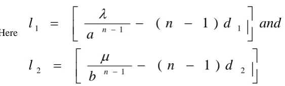
n nHere
2 1
2
1 1
1
)
1
(
)
1
(
d
n
b
l
and
d
n
a
l
n n
4. Empirical Results and Conclusions
For given fixed values of , , , r, , C, Cr the optimal replacement policy N* is calculated as follows:
Let, =15, a=0.69, b=1.04, =3, r=18, =4, T=40, =200, d1=1.05, d2=0.9, Cr=50, =3, C=5000
Table 1 : N Vs C(N)
N C(N) N C(N)
1 -11.878972 26 -17.127275
2 269.410309 27 -17.364845
3 315.164001 28 -17.538441
4 297.356415 29 -17.665060
5 258.945160 30 -17.757261
6 215.546143 31 -17.824299
7 173.761078 32 -17.872969
8 136.393799 33 -17.908257
9 104.412758 34 -17.933811
10 77.850868 35 -17.952293
11 56.275745 36 -17.965647
12 39.053028 37 -17.975285
13 25.495729 38 -17.982233
14 14.945923 39 -17.987238
15 6.815018 40 -17.990841
16 0.599144 41 -17.993431
17 -4.119857 42 -17.995293
18 -7.681098 43 -17.996628
19 -10.354709 44 -17.997587
20 -12.352837 45 -17.998274
21 -13.840179 46 -17.998766
22 -14.943392 47 -17.999119
23 -15.759094 48 -17.999371
24 -16.360504 49 -17.999550
Conclusion:
1 From the table 1 & graph 1, we see that C(3) = 315.164001 is the maximum of the long-run expected reward cost per unit time of the system i.e the optimal policy is N* = 3 and we should replace the system at the time of 3rd failure.
2 By examining for various values of parameters, we can comment that the optimal number of failures
does not affect much for a considerable change in a & b but there is substantial change in long-run expected reward cost per unit time C(N) of the system.
References:
[1] Abdel-Hameed,M., “ Optimum Replacement of system subject to shocks”, Journal of Applied probability, Vol.No.23, 1986, pp 107-114.
[2] Borwn, M., and Proschan, F., “Imperfect Repair”, Journal of Applied Probability, Vol.20, 1983, PP 851-859.
[3] Block,H.W.,Borges,W.S., Savits,T.H., “A general age replacement model with minimal repair”, Naval Research Logistics, Vol.No.35, 1988, pp 365-372.
[4] Barlow, R.E., and Proschan, F., “ Statistical theory of Reliability and life testing”, Holt. Rinehart, Winston, 1975.
[5] Esary, J.D., Marshall, A.W., and Proschan, F., “ Shock Models and wear process”, Annals of probability, Vol.1, 1973, pp 627-650. [6] Feldman,R.M., “ Optimal replacement with semi-Markov shock models”, Journal of Applied probability, Vol. No.13, 1976, pp
108-117.
[7] Gary Gottlieb., “ Optimal Replacement model for shock Models with General failure Rate”, operations Research, Vol.30, No.1, 1982, pp 82-92.
[8] Leung ,K.N.F.,and Lee, Y.M., “ Using geometric processes to study maintenance problems for engines”, International journal of Industrial Engineering, Vol.5, 1998, pp 316-323.
[9] Lam Yeh., “An optimal Repairable Replacement model for Deteriorating systems”, Journal of Applied probability, Vol No. 28, 1991, pp 843-851.
[10] Lam Yeh., “Geometric Processes and Replacement Problems”, Acta Mathematicae Applicatae Sinica, Vol.4, 1988 a, pp 366-377. [11] Lam Yeh., “A Note on the Optimal Replacement Problem”, Advanced Applied Probability, Vol.20, 1988 b, pp 479-482. [12] Phelps, R.I., “ Replacement policies under minimal repair”, Journal of operational Research society, Vol.32, 1981, pp 549-554. [13] Shanthi Kumar, J.G., and Sumita, U., “General shock models associated with correlated Renewal sequences”, Journal of Applied
probability, Vol.20, 1983, pp 600-619.
[14] Park,K.S., “Optimal Number of Minimal Repairs before Replacement”, IEEE Transactions on Reliability, vol. R-28, No.2, Jun 1979, pp 137-140.
[15] Ross, S.M., “Applied Probability Models with optimization Applications”, San Francisco, Holden-Day, 1970.
[16] Ravichandra Kumar T.C and Y.Krishna Reddy, “optimal Repair replacement policy for two – type failures model with α – series process”, proceedings of A.P. Akademi of sciences, Vol.12(3), 2008, pp 301-306.
[17] Stanely, A.D.J., “On Geometric Processes and Repair Replacement Problems”, Microelectronics Reliability, Vol.33, 1993, pp489-491. [18] Shooman, M.L., “Probabilistic Reliability-An Engineering Approach”, McGraw Hill, New York, 1968.
[19] Stadje, W., and Zuckerman, D., “Optimal Strategies for some Repair Replacement Models”, Advanced Applied Probability, Vol.22, 1990, pp 641-656.
[21] Zuckerman, D., “Optimal stopping in semi-Markov shock model”, Journal of Applied probability, Vol.15, 1978, pp 629-634. [22] Zhang, Y.L., Yam, R.C.M., and Zuo, M.J., “Optimal Replacement Policy for a Multistate Repairable System”, Journal of the
Operational Research Society, Vol. No.53, 2002, pp 336-341.