The CALIPSO version 4 automated aerosol classification and lidar
ratio selection algorithm
Man-Hae Kim1, Ali H. Omar2, Jason L. Tackett3, Mark A. Vaughan2, David M. Winker2, Charles R. Trepte2, Yongxiang Hu2, Zhaoyan Liu2, Lamont R. Poole3, Michael C. Pitts2, Jayanta Kar3, and Brian E. Magill3
1NASA Postdoctoral Program (USRA), Hampton, VA, USA 2NASA Langley Research Center, Hampton, VA, USA 3Science Systems and Applications, Inc., Hampton, VA, USA
Correspondence:Man-Hae Kim ([email protected]) Received: 21 May 2018 – Discussion started: 26 June 2018
Revised: 26 September 2018 – Accepted: 1 October 2018 – Published: 12 November 2018
Abstract.The Cloud-Aerosol Lidar with Orthogonal Polar-ization (CALIOP) version 4.10 (V4) level 2 aerosol data products, released in November 2016, include substantial improvements to the aerosol subtyping and lidar ratio se-lection algorithms. These improvements are described along with resulting changes in aerosol optical depth (AOD). The most fundamental change in the V4 level 2 aerosol prod-ucts is a new algorithm to identify aerosol subtypes in the stratosphere. Four aerosol subtypes are introduced for strato-spheric aerosols: polar stratostrato-spheric aerosol (PSA), volcanic ash, sulfate/other, and smoke. The tropospheric aerosol sub-typing algorithm was also improved by adding the following enhancements: (1) all aerosol subtypes are now allowed over polar regions, whereas the version 3 (V3) algorithm allowed only clean continental and polluted continental aerosols; (2) a new “dusty marine” aerosol subtype is introduced, represent-ing mixtures of dust and marine aerosols near the ocean sur-face; and (3) the “polluted continental” and “smoke” sub-types have been renamed “polluted continental/smoke” and “elevated smoke”, respectively. V4 also revises the lidar ra-tios for clean marine, dust, clean continental, and elevated smoke subtypes. As a consequence of the V4 updates, the mean 532 nm AOD retrieved by CALIOP has increased by 0.044 (0.036) or 52 % (40 %) for nighttime (daytime). Li-dar ratio revisions are the most influential factor for AOD changes from V3 to V4, especially for cloud-free skies. Pre-liminary validation studies show that the AOD discrepancies between CALIOP and AERONET–MODIS (ocean) are re-duced in V4 compared to V3.
1 Introduction
The Cloud-Aerosol Lidar with Orthogonal Polarization (CALIOP) flown aboard the Cloud-Aerosol Lidar and In-frared Pathfinder Satellite Observations (CALIPSO) plat-form has been providing unique vertical profile measure-ments of the Earth’s atmosphere on a global scale since June 2006 (Winker et al., 2010). Data products derived from the CALIOP measurements are distributed worldwide from the Atmospheric Science Data Center (ASDC) located at the Na-tional Aeronautics and Space Administration (NASA) Lan-gley Research Center (LaRC). In addition to detailed spatial and optical properties of detected layers, CALIOP also pro-vides essential information on layer types for both clouds and aerosols.
op-tical properties. The aerosol lidar ratio, a key parameter for the extinction retrieval, is determined for each aerosol sub-type based on measurements, modeling, and the cluster anal-ysis of a multiyear Aerosol Robotic Network (AERONET) dataset (Omar et al., 2005, 2009). Because the lidar ratio is one of the largest sources of uncertainty in the CALIOP aerosol optical depth (AOD) estimates, the CALIOP aerosol classification and lidar ratio selection algorithm plays a criti-cal role in the aerosol extinction retrieval and resulting AOD (Young et al., 2013).
In version 3 (V3) and earlier, the CALIOP level 2 aerosol classification and lidar ratio selection algorithm defined six aerosol types: clean marine, dust, polluted continental, clean continental, polluted dust, and smoke (Omar et al., 2009). Each type is assigned an extinction-to-backscatter ratio (i.e., lidar ratio) with an associated uncertainty that defines the limits of its expected natural variability. Since the V3 re-lease, several limitations of the V3 aerosol subtyping algo-rithm have come to light. For instance, mixtures of dust and marine aerosol were frequently classified as polluted dust (Burton et al., 2013), which is intended to be a mixture of dust and smoke or urban pollution. In polar regions, Asian dust and smoke from boreal fires were forced to be classi-fied as either clean continental or polluted continental, the only aerosol subtypes allowed over snow, ice, or tundra. The algorithm for identifying smoke also caused some layers at the bases of elevated smoke plumes to be misclassified as clean marine (Nowottnick et al., 2015). Finally, all features detected above the tropopause were generically classified as “stratospheric features” and were not given aerosol subtypes, thereby missing an opportunity to identify volcanic aerosol in the stratosphere.
The conclusions from numerous studies assert that the AOD reported in the CALIOP V3 data products typically un-derestimates coincident AOD measurements and/or retrievals acquired using various spaceborne, airborne, and ground-based instruments (e.g., Redemann et al., 2012; Schuster et al., 2012; Kim et al., 2013; Omar et al., 2013; Rogers et al., 2014). Additional CALIOP analyses using opaque water clouds as a constraint in the retrieval (Hu, 2007) show sim-ilar results (Liu et al., 2015). However, the Moderate Reso-lution Imaging Spectroradiometer (MODIS) AOD retrievals (collection 5) are subject to several sources of error, which mostly tend to produce high biases in AOD (Kittaka et al., 2011). Campbell et al. (2012) compared with the US Navy Aerosol Analysis and Prediction System (NAAPS), which assimilates a quality-screened version of MODIS AOD, and find that the V3 CALIOP AOD is consistent with NAAPS over ocean and somewhat higher over land.
There are two primary sources for the CALIOP AOD differences relative to other measurements and retrievals: aerosol layer detection failures and inaccurate lidar ratios. Rogers et al. (2014) compared CALIOP AOD with NASA LaRC airborne High Spectral Resolution Lidar (HSRL) and found that the undetected aerosols in the free troposphere
in-troduce a mean underestimate of 0.02 in the CALIOP column AOD in the dataset examined. Kim et al. (2017) retrieved aerosol extinction for the undetected aerosol layers and found a global mean undetected layer AOD of 0.031. Toth et al. (2018) reported that 45 % of daytime cloud-free V3 level 2 aerosol profiles have no aerosol detected within the pro-file (AOD =0). They found the mean collocated MODIS and AERONET AODs at 550 nm are near 0.06 and 0.08, re-spectively, for the CALIOP profiles without aerosols. Sev-eral other studies also suggest that the weakly backscattering aerosols that are undetected by CALIOP’s layer detection al-gorithm can contribute to a low CALIOP AOD estimate rel-ative to other sensors (Kacenelenbogen et al., 2011, 2014; Thorsen et al., 2017). Whereas layer detection failure always contributes to low bias, misclassification of aerosol subtypes and inaccurate aerosol lidar ratios can result in both high and low biases in CALIOP AOD. Burton et al. (2013) compared the CALIOP V3 aerosol subtype product with NASA LaRC airborne HSRL measurements. They compared 109 under-flights of the CALIOP orbit track and found that 80 % of the CALIOP desert dust layers, 62 % of the marine layers, and 54 % of the polluted continental layers agreed with HSRL classification results. However, the agreement was less for smoke (13 %) and polluted dust (35 %) layers. Recent stud-ies suggest that the lidar ratios assigned by the V3 CALIOP aerosol classification and lidar ratio selection algorithm are at least partially responsible for biases in the CALIOP V3 AOD for clean marine (Bréon, 2013; Rogers et al., 2014; Dawson et al., 2015) and dust aerosols (Burton et al., 2012; Schuster et al., 2012; Amiridis et al., 2013; Nisantzi et al., 2015; Liu et al., 2015).
The CALIOP version 4.10 (V4) level 2 aerosol data prod-ucts, released in November 2016, contain substantial updates to aerosol type classification and to aerosol lidar ratio assign-ments, made in response to many of the results reported in the studies described above. The primary purpose of this pa-per is to introduce the V4 updates in the CALIOP level 2 aerosol subtyping algorithms and changes to the character-istic lidar ratios for different aerosol subtypes. This is dis-cussed in Sect. 2. The resulting AOD differences between V3 and V4 are investigated in Sect. 3 by categorizing the factors that can contribute to the AOD changes. Lastly, in Sect. 4, we compare CALIOP AOD with AERONET and MODIS for both versions as an initial validation of the CALIOP V4 AOD.
2 Algorithm updates for CALIOP version 4 aerosol level 2 products
tropo-Polluted dust
Polluted continental/ smoke
Clean continental Elevated smoke
Marine
Ztop > 2.5 km
γ’ > 0.01
Yes γ’ > 0.0005
δpest > 0.20
No
No
Ztop > 2.5 km
Yes γ’ > 0.0015
Yes No
Desert dust Yes
Yes No
No δpest > 0.075
Yes
Surface type Snow/ice
tundra? No
Clean continental
Desert
No
Yes
Land Ocean
No
Surface type Zbase > 2.5 km
Dusty marine
Polluted continental
Land Yes
Yes No
Ocean
Yes No
Is the layer wholly above the MBL?
Version 3
Version 4
Ztop, Zbase : layer top and base altitude
δpest < 0.05 Yes
No
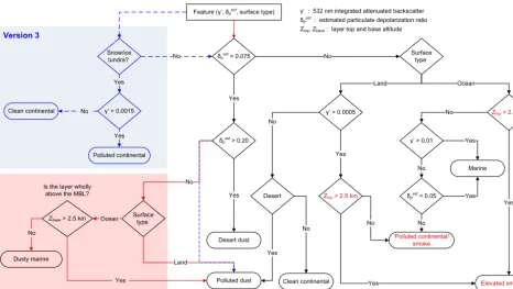
Figure 1.Flowchart of the CALIPSO aerosol subtype selection scheme for tropospheric aerosols. The blue-shaded region and blue-dotted arrows are used in V3 but removed in V4. The red-shaded region and solid red arrows are newly added in V4. The nomenclatures for “polluted continental” and “smoke” are revised to “polluted continental/smoke” and “elevated smoke” in V4. The definition for “elevated” is revised in V4 to mean layers with tops higher than 2.5 km above ground level (see Sect. 2.1.3).
sphere and the addition of new aerosol subtypes to classify aerosol layers newly identified in the stratosphere. Because the cloud aerosol discrimination (CAD) algorithm is now ap-plied to all layers detected (Liu et al., 2018), those features that were previously classified as generic “stratospheric” lay-ers in V3 and earlier are now identified as either clouds or aerosols. Consequently, the V4 level 2 aerosol subtyping al-gorithm now distinguishes between tropospheric and strato-spheric aerosols. An entirely new algorithm has been imple-mented to identify aerosol subtypes in the stratosphere, and the algorithm for identifying tropospheric aerosol types has been substantially updated. The changes made to the tropo-spheric algorithm are described in detail first, followed by details on the new stratospheric aerosol subtyping algorithm. 2.1 Aerosol subtypes in the troposphere
The CALIOP V3 aerosol classification algorithm uses alti-tude, location, surface type, estimated particulate depolariza-tion ratio (δpest), and integrated attenuated backscatter (γ0) to identify the aerosol subtype (Omar et al., 2009). Figure 1 shows the decision tree used to determine the V3 and V4 tro-pospheric aerosol subtypes. The major updates implemented in the V4 tropospheric aerosol subtyping algorithm include introducing the dusty marine aerosol subtype (by adding the red-shaded region in Fig. 1), allowing all aerosol subtypes
over polar regions (by removing the blue-shaded region in Fig. 1), and revising the operational definitions for the pol-luted continental and smoke aerosol types.
At this time the integrated attenuated color ratio (χ0=
γ10640/γ5320) is not used for aerosol subtyping in the tropo-sphere because the low signal-to-noise ratio (SNR) for opti-cally thin layers, especially in the daytime, makes it an in-consistent discriminator among tropospheric aerosol types. However, it is useful for stratospheric aerosol typing in which the number of types is fewer (Sect. 2.2).
2.1.1 A new aerosol subtype: dusty marine
In V4, a new dusty marine aerosol type is introduced to identify mixtures of dust and marine aerosol and thus ac-count for the frequent occurrence of mixtures of dust and marine aerosols that are misclassified as polluted dust over global oceans in V3. Dusty marine occurs most frequently when Saharan dust is transported across the Atlantic Ocean and settles into the marine boundary layer (MBL) as it ap-proaches North and Central America (Liu et al., 2008; Groß et al., 2016; Kuciauskas et al., 2018). In V3, many of these layers are misclassified as polluted dust, an aerosol type in-tended to represent mixtures of dust +smoke and dust+
(a) Polluted dust, V3 Night (b) Polluted dust, V3 Day
(c) Polluted dust, V4 Night (d) Polluted dust, V4 Day
(e) Dusty marine, V4 Night (f) Dusty marine, V4 Day
60°
30°
0°
−30°
−60°
60°
30°
0°
−30°
−60°
60°
30°
0°
−30°
−60°
−180° −120° −60° 0° 60° 120° 180° −180° −120° −60° 0° 60° 120° 180°
90 80 70 60 50 40 30 20
0 10 100
Frequency (%)
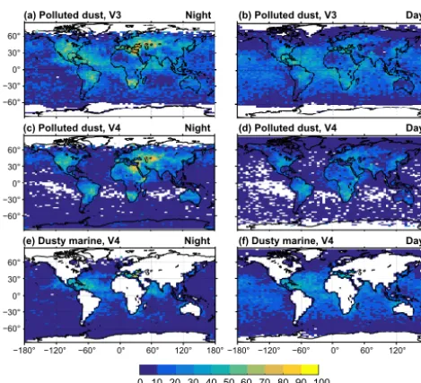
Figure 2.Frequency of occurrence of aerosol samples classified as polluted dust in V3 at night and during the day(a, b), polluted dust in V4 at night and during the day(c, d)and dusty marine in V4 at night and during the day(e, f). June–August 2007.
during CALIPSO validation flights over the Caribbean Sea, Burton et al. (2013) compared CALIOP V3 aerosol classi-fications with measurements made by the NASA LaRC air-borne HSRL on the NASA B200 aircraft. For those layers that CALIOP V3 classified as polluted dust, the HSRL mea-sured a median lidar ratio of 35 sr, thus strongly suggest-ing that these aerosols were a combination of dust+marine aerosol, and not the combination of dust+smoke modeled by the CALIOP polluted dust type. As shown in Fig. 2a, 40 % to 50 % of aerosol samples over the Caribbean in JJA at night are classified as polluted dust in V3. During the daytime in V3 (Fig. 2b), polluted dust accounts for 10 % to 30 % of aerosol samples identified over remote oceanic regions (e.g., the South Pacific Ocean) where the occurrence of mixtures of dust and smoke is less probable.
The polluted dust classification occurred in V3 because these layers are mildly depolarizing, having estimated par-ticulate depolarization ratios (δestp ) between 0.075 and 0.20 (Omar et al., 2009). The estimated particulate depolariza-tion ratio is the layer-integrated volume depolarizadepolariza-tion ratio, which is corrected to account for the molecular contribution, defined as
δpest=δv[(Rmas−1) (1+δm)+1]−δm
(Rmas−1) (1+δm)+δm−δv
, (1)
whereδvis the layer-integrated volume depolarization ratio,
Rmas is the mean attenuated scattering ratio, and δm is the molecular depolarization ratio (Omar et al., 2009). Here,δv
is defined as
δv=
Pztop
zbaseβ⊥0(z)
Pztop
zbase
βk0(z)
, (2)
wherezis altitude and the subscripts “top” and “base” refer to the top and base of the detected aerosol layer.
When a dust layer, having δpest>0.20, mixes with non-depolarizing marine aerosol, the layer-averaged δpest de-creases below 0.20 and the aerosol is classified as polluted dust in V3. This explains the enhanced frequency of V3 pol-luted dust classifications over the Caribbean in JJA (Fig. 2a). In other oceanic regions where dust + marine or dust +
smoke mixtures are less probable (again, the remote South Pacific Ocean), the frequency of polluted dust is overesti-mated in V3 for at least two reasons. First, δpest is a noisy quantity that is asymmetrically distributed, with a large pos-itively skewed tail that can be considerably increased by solar background noise during the daytime. Additionally, occasional high biases can arise from residual single-shot-resolution cloud contamination within the MBL. This makes the 0.075 lowerδestp threshold easier to exceed in these situa-tions. Second,δestp is overestimated in V3 because attenuation from overlying layers was not accounted for in theδestp com-putation (Burton et al., 2013) in V3. This oversight has been corrected in V4.
To identify dust + marine aerosol mixtures in V4, dusty marine layers are defined as moderately depolarizing (0.075<δestp <0.20) aerosol layers over ocean having base al-titudes below 2.5 km above mean sea level (an upper limit for the MBL; Winning et al., 2017). After implementation of this new aerosol subtype, the frequency of oceanic layers classified as polluted dust decreased substantially. Given that the CALIOP polluted dust subtype is explicitly modeled as a mixture of dust and smoke (Omar et al., 2009), the V4 spatial distributions of polluted dust over the Caribbean and remote Pacific Ocean shown in Fig. 2c and d present a more likely scenario than the V3 distributions shown in Fig. 2a and b. A total of 30 %–50 % of aerosol samples over the Caribbean are classified as dusty marine in JJA as shown in Fig. 2e–f. Note that the dusty marine frequency is enhanced over re-mote oceanic regions during the daytime (Fig. 2f). This is due to the noisiness ofδestp in daytime. The AOD differences from misclassifying pure marine (lidar ratio of 23 sr) as dusty marine (37 sr) are substantially smaller than they would oth-erwise be if these same layers were instead misclassified as polluted dust (55 sr).
2.1.2 Aerosol subtypes in polar regions
industri-Dust
(b) Depolarization ratio 532 nm
(c) Version 3 aerosol subtypes
(d) Version 4 aerosol subtypes Polluted continental Clean continental Dust Polluted dust 10-2 10-3 10-4 15 10 5 0 A lt it ude ( km ) 20 15 10 5 0 A lt it ude ( km ) 20 15 10 5 0 A lt it ude ( km ) 20 15 10 5 0 A lt it ude ( km )
1 = marine, 2 = dust, 3 = polluted continental/smoke, 4 = clean continental, 5 = polluted dust, 6 = elevated smoke, 7 = dusty marine
Lat (°) Long (°) 77.04 -177.84 66.28 161.87 54.55 153.61 42.55 148.72 30.47 145.16 0.0 1.0 0.9 0.8 0.7 0.6 0.5 0.4 0.3 0.2 0.1 6 5 4 3 2 1 N/A 6 5 4 3 2 1 N/A 7 71.88 199.23 60.46 157.07 48.57 150.93 36.50 146.83
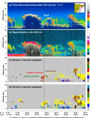
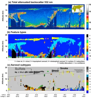
Figure 3.CALIOP observations of dust plume on 22 March 2010 between 16:11 and 16:25 UTC.(a)Total attenuated backscatter at 532 nm,
(b)depolarization ratio at 532 nm, and aerosol subtypes in(c)V3 and(d)V4. The white dashed ellipse shows dust plume and the black dashed line represents the boundary for “snow/ice, tundra” used for polar regions in V3.
alized areas transported poleward (Stohl, 2006; Stone et al., 2008). During the spring phase of the ARCTAS campaign (Jacob et al., 2010), however, the poleward transport of mul-tiple plumes of Asian dust and smoke from boreal fires was observed, highlighting the importance of these other aerosol types. The contribution of smoke to the aerosol found in the Arctic – primarily from boreal forest fires and high-latitude agricultural fires – is now well documented (e.g., Stohl et al., 2007; Warneke et al., 2010; Di Pierro et al., 2011; Markow-icz et al., 2016). Records in polar ice and snow cores show that dust has been transported to the Arctic and Antarctic since geologic times (e.g., Lunt and Valdes, 2001; Fischer et al., 2007). While there are dust sources at high latitudes in both the Northern Hemisphere (Alaska, Canada, Green-land, and Iceland) and Southern Hemisphere (Antarctica, New Zealand, and Patagonia) (Bullard et al., 2016), they are
(Fig. 3b) with the white dashed ellipse. However, the V3 al-gorithm identifies the plume as dust/polluted dust at latitudes less than 56◦N but as polluted continental/clean continental above 56◦N (Fig. 3c). The sea surface changes from open water to ice at this point, and hence the aerosol subtyping, is forced by the V3 polar region loop (Fig. 1). In V4, this plume is correctly classified as dust (Fig. 3d). Note too that the V3 analysis fails to detect a substantial fraction of the plume, whereas the V4 algorithm captures the whole plume well (Fig. 3d), thus demonstrating the layer detection improve-ments in V4 (Sect. 3.2).
2.1.3 Revised aerosol subtype: elevated smoke and polluted continental/smoke
The interpretation and nomenclature of layers identified in V3 as smoke and polluted continental have been revised in V4. As in previous versions, elevated non-depolarizing aerosols are assumed to be smoke that has been injected above the planetary boundary layer (PBL). The definition for elevated is revised in V4 to mean layers with tops higher than 2.5 km above ground level (i.e., a simple approximation of a region above the PBL; McGrath-Spangler and Denning, 2013). For clarity, the name of the smoke aerosol subtype is changed to “elevated smoke” to emphasize that these lay-ers are identified as smoke because they are elevated above the PBL. Within the PBL, the optical properties measured by CALIOP (depolarization and color ratio) are practically identical for the smoke and polluted continental subtypes, making them indistinguishable. To acknowledge the opti-cal similarity of polluted continental and smoke, the name of this aerosol type is changed in V4 to “polluted continen-tal/smoke”. The V4 lidar ratios used in the CALIOP retrieval algorithm are identical for polluted continental/smoke and el-evated smoke (70 sr at 532 nm and 30 sr at 1064 nm). How-ever, one limitation of identifying smoke layers according to altitude is that pollution lofted by convective processes or other vertical transport mechanisms can be misclassified as elevated smoke.
2.2 Stratospheric aerosols
In V4, the CAD algorithm is applied at all altitudes, includ-ing in the stratosphere. By contrast, previous versions only applied the CAD algorithm below the tropopause, classify-ing layers detected above the tropopause as stratospheric fea-tures rather than as clouds or aerosols. As a consequence, aerosol existing above the tropopause was not identified ex-plicitly as aerosol. However, it is well documented that cer-tain aerosol types exist in the stratosphere. Volcanic eruptions inject ash and sulfate to high altitudes (e.g., Vernier et al., 2011; Bourassa et al., 2012). Smoke due to intense combus-tion or from pyro-cumulonimbus events can also breach the tropopause (e.g., Fromm et al., 2005, 2010; Trentmann et al., 2006). In the polar winter, polar stratospheric clouds (PSCs)
form and the PSC composed of supercooled ternary solution (STS) is an aerosol (Pitts et al., 2009). In V4, features iden-tified by the CAD algorithm as aerosol having 532 nm atten-uated backscatter centroids (Garnier et al., 2015) above the tropopause from the Modern-Era Retrospective analysis for Research and Applications version 2 (MERRA-2) reanaly-sis data (Gelaro et al., 2017) outside of the polar regions are classified as “stratospheric aerosols”. Distinguishing among the different types of stratospheric aerosol relies primarily on latitude, temperature, and the measured properties of each layer:γ0andδestp at 532 nm andχ0.
V4 identifies four stratospheric aerosol subtypes: vol-canic ash, sulfate/other, elevated smoke, and polar strato-spheric aerosol (PSA). Volcanic ash is defined as an aspher-ical volcanic aerosol that depolarizes the 532 nm backscat-ter, whereas sulfate/other is defined primarily as a non-depolarizing volcanic aerosol. The “other” component of this aerosol type is the catchall for stratospheric aerosol layers that are either weakly scattering or cannot be classified as any other type within the stratospheric aerosol algorithm. Weakly scattering layers are not evaluated by the strato-spheric aerosol subtyping algorithm because the noisy values ofδestp andχ0at low signal levels inhibit robust classifications with the threshold-based technique employed. The PSA sub-type is introduced in V4 to assign a reasonable aerosol sub-type for features detected in the polar regions during polar win-ter and subsequently classified as aerosol by the CAD algo-rithm due to their low values ofχ0andγ0. Comparison with the CALIOP L2 PSC mask product shows that PSAs are spa-tially correlated with the STS PSC composition class (Pitts et al., 2009; Liu et al., 2018). However, layers assigned the PSA subtype should be interpreted carefully. For in-depth studies, the CALIPSO team recommends using the CALIOP L2 PSC mask product for analyses related to PSC composition since it is a more specialized product (Pitts et al., 2009).
Figure 4.Flowchart of the CALIPSO aerosol subtype selection scheme for stratospheric aerosols.
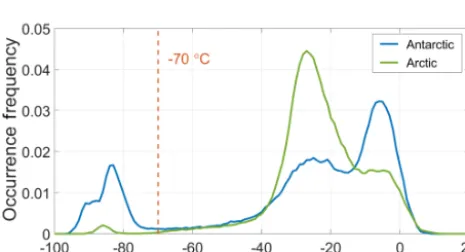
Figure 5.Occurrence frequency of mid-layer temperatures for V4 aerosol layers detected poleward of 50◦during PSC season; June– September 2008 for the Antarctic and December 2007–February 2008 for the Arctic at night.
Next, in order to discriminate between volcanic ash, sul-fate, and elevated smoke, the stratospheric aerosol typing algorithm evaluates layer-averaged δestp andχ0 against em-pirically derived thresholds. These thresholds were derived from frequency distribution analysis ofδpestandχ0 measure-ments obtained from a manually identified subset of volcanic ash, sulfate, and high-altitude smoke layers (Fig. 6). The number of unique layers detected by CALIOP, geophysical events, and dominant aerosol types contributing to this sub-set are summarized in Table 1. Note that, as previously men-tioned, weakly scattering stratospheric aerosol layers (layers with γ0<0.001 sr−1) are directly classified as sulfate/other
due to their low SNR. As shown in Fig. 6a–c, volcanic ash and volcanic sulfate are fairly well separated with respect toδpest, with ash typically havingδestp >0.15 and sulfate with 0.075<δestp <0.15. Smoke layers are less depolarizing than volcanic ash (Fig. 6d), withδestp <0.15. However, smoke lay-ers can be either non-depolarizing or moderately depolariz-ing (Fig. 6e–f). An example of a moderately depolarizdepolariz-ing smoke event is the February 2009 “Black Saturday” Aus-tralian bush fire for which δpest frequently exceeded 0.10. Non-depolarizing smoke layers (δpest<0.075) typically have
χ0>0.5, whereasχ0is more frequently lower for moderately depolarizing smoke layers (0.075<δestp <0.15). Based on this analysis, the stratospheric aerosol typing algorithm depicted in Fig. 4 was constructed using the thresholds indicated by the red lines in Fig. 6.
The following examples demonstrate the strengths and limitations of the stratospheric aerosol typing algorithm. Vol-canic ash is well separated from the other types in terms of
sub-Table 1.Number of layers detected by CALIOP used to determine V4 stratospheric aerosol typing thresholds. The dominant aerosol type for volcanic events is determined according to the references given in the table.
Nlayers Geophysical event Dominant aerosol type
2274 Puyehue-Cordón Caulle eruption, June 2011 Volcanic ash (Bignami et al., 2014) 69 Okmok eruption, July 2008 Volcanic ash (Prata et al., 2010) 58 Chaitén eruption, May 2008 Volcanic ash (Prata et al., 2010) 2439 Kasatochi eruption, August 2008 Volcanic sulfate (Krotkov et al., 2010)
256 Nabro, June 2011 Volcanic sulfate (Theys et al., 2013)
813 Siberian fires, May–June 2012 Smoke
399 Canadian fires, July–August 2007 Smoke
1624 Australian bush fire, February 2009 Smoke, depolarizing (de Laat et al., 2012)
161 Canadian fires, May 2007 Smoke, depolarizing
Figure 6.Two-dimensional frequency distributions of attenuated total color ratio and estimated particulate depolarization ratio for layers in Table 1. Distributions are normalized independently by the sum of samples in the subset:(a)all volcanic layers,(b)volcanic sulfate,
(c)volcanic ash,(d)all smoke layers,(e)non-depolarizing smoke, and(f)depolarizing smoke. Only layers having integrated attenuated backscatter>0.001 sr−1contribute. Red dashed lines denote the V4 stratospheric aerosol typing thresholds.
types that do not include ash. Because the noise-broadened distributions ofδestp for ash and dust measured by CALIOP have very similar characteristics, we know of no robust way to discriminate the two within the troposphere (Winker et al., 2012). However, the lidar ratio assigned for ash is identical to that for dust (Table 2) so potential misclassifications will have minimal impact on the extinction products.
Figure 8 presents a scene in which the bulk of the Nabro volcano plume from June 2011 (Theys et al., 2013) is cor-rectly classified as sulfate. In this example, most of the layer hasγ0>0.001 and low depolarization, yielding a sulfate clas-sification for the more optically thick segments. However, a small number of layers within the plume are misclassified as smoke. This is expected because of the overlap in the fre-quency distributions of δpestandχ0for sulfate (Fig. 6b) and
(b) Feature types
10-2
10-3
10-4
1 = clear air, 2 = cloud, 3 = tropospheric aerosol, 4 = stratospheric aerosol, 5 = surface, 6 = subsurface, 7 = totally attenuated, L = no confidence
7
6
5 4
3
3(L)
2
2(L)
1 15
10
5
0
20
15
10
5
0
Altit
ud
e
(km)
Altit
ud
e
(km)
1 = marine, 2 = dust, 3 = polluted continental/smoke, 4 = clean continental, 5 = polluted dust, 6 = elevated smoke, 7 = dusty marine, 8 = PSC aerosol, 9 = volcanic ash, 10 = sulfate/other -41.8
126.4 -47.8 124.3
-53.8 121.7
-59.7 118.3
-65.5 113.8
-71.1 106.9
-76.4 95.1
-80.5 72.0
-81.8 32.4 Lat (°)
Long (°)
Sulfate
Ash
PSCaerosol
(c) Aerosol subtypes
Dust
Tropopause (approx.)
10
9 8
7 6 5 4 3 2 1 20
15
10
5
0
Altit
ud
e
(km)
(km
-1
sr
-1
)
Figure 7. CALIOP observations of the Puyehue-Cordón Caulle volcano plume on 20 June 2011 between 16:50 and 17:00 UTC.
(a) Total attenuated backscatter at 532 nm, (b) V4 feature type classification, and (c) V4 aerosol subtypes, where the dashed line indicates the approximate location of the tropopause. The satellite ground track is indicated by the green section on the inset map in panel (a). Additional imagery for this scene, including 532 nm depolarization ratios and attenuated backscatter color ra-tios, can be found at https://www-calipso.larc.nasa.gov/products/lidar/browse_images/show_detail.php?s=production&v=V4-10&browse_ date=2011-06-20&orbit_time=16-22-13&page=3&granule_name=CAL_LID_L1-Standard-V4-10.2011-06-20T16-22-13ZN.hdf (last ac-cess: 26 September 2018).
tropopause as a generic stratospheric layer without applying any further subtyping. In V4, these same layers are most of-ten correctly classified as aerosols by the new CAD algorithm (Liu et al., 2018). Similarly, the new stratospheric aerosol subtyping algorithm is largely successful in identifying the correct aerosol subtype.
2.3 Subtype Coalescence Algorithm for AeRosol Fringes (SCAARF)
In previous data releases, “fringes” at the bases of dense aerosol plumes were at times misclassified as an aerosol sub-type inconsistent with the parent plume. These fringes typi-cally lie below rapidly attenuating aerosol layers and are de-tected at the coarser horizontal resolutions (20 and 80 km) employed by CALIOP’s iterated, multi-resolution layer de-tection scheme (Vaughan et al., 2009). An example is shown in Fig. 10a–b, in which fringes at the base of an elevated
smoke plume are misclassified as clean marine aerosol. In this case, the fringes are misclassified because the layers are non-depolarizing and have top altitudes just below the 2.5 km altitude threshold that would have otherwise caused them to be correctly classified as elevated smoke according to the re-vised definition of elevated in V4 (Sect. 2.1.3). Given that this is an elevated plume not in contact with any aerosol be-neath, it is reasonable to expect that the misclassified fringes at the base of the plume have the same aerosol subtype as the adjacent smoke layers. This same argument can be made for other aerosol types that contiguously span large horizon-tal distances (e.g., dust plumes, marine aerosol, volcanic ash, and volcanic sulfate).
Table 2.Aerosol lidar ratios with expected uncertainties for tropospheric and stratospheric aerosol subtypes at 532 and 1064 nm in CALIOP version 3 and 4 aerosol retrieval algorithms.
Aerosol subtype S532(sr) S1064(sr)
Tropospheric aerosols
V3 V4 V3 V4
Clean marine 20±6 23±5 45±23 23±5
Dust 40±20 44±9 55±17 44±13
Polluted continental/smoke 70±25 70±25 30±14 30±14 Clean continental 35±16 53±24 30±17 30±17 Polluted dust 55±22 55±22 48±24 48±24 Elevated smoke 70±28 70±16 40±24 30±18
Dusty marine – 37±15 – 37±15
V4 stratospheric aerosols
Polar stratospheric aerosol 50±20 25±10
Volcanic ash 44±9 44±13
Sulfate/other 50±18 30±14
Smoke 70±16 30±18
lower fringes to match the dominant subtype of the adjacent overlying layers. According to SCAARF, fringes are defined as aerosol layers detected at 20 or 80 km horizontal resolu-tions that are vertically adjacent to the base(s) of aerosol lay-ers detected at finer spatial resolution (i.e., they are adjacent to more strongly scattering features). At least 50 % of the hor-izontal extent of the fringe candidate must be in contact with aerosol overhead. SCAARF is applied to all tropospheric and stratospheric aerosol layers meeting this fringe criteria. The dominant adjacent aerosol subtype is determined from the number of 5 km resolution samples vertically adjacent to the fringe. When two adjacent aerosol subtypes exist with equal frequency (i.e., neither is dominant in terms of number), the fringe is changed to match the subtype of the adjacent lay-ers that are most similar to the fringe in terms ofδestp andχ0. This is the subtype with the minimum Euclidian distanceri
betweenδ¯estp andχ¯0of the parent andδestp andχ0of the fringe; i.e.,
ri =
r
δpest,fringe− ¯δestp,subtypei 2
+ χ0
fringe− ¯χ0subtypei
2 ,
for i∈ [1,2]. (3)
Here, δ¯pest,subtypei and χ¯0subtypei are the average values of
δpest andχ0 for all adjacent layers having unique subtypes
i∈ [1,2]. The fringe is changed to match subtypei where
ri =minimum(r1, r2). If three or more unique subtypes are
adjacent to the fringe with equal frequency, SCAARF is not applied.
In effect, SCAARF aids in vertically homogenizing aerosol subtype classification along plume bases. Figure 10c demonstrates that the fringes misclassified as clean ma-rine have been correctly classified as elevated smoke after SCAARF is implemented. Similar improvement occurs for
volcanic ash layers straddling the tropopause. Lower fringes of these plumes below the tropopause would otherwise be misclassified as dust (Sect. 2.2), yet SCAARF helps retain the volcanic ash classification.
2.4 Aerosol lidar ratios in version 4
Table 2 shows the lidar ratios that characterized the V3 aerosol types and the revised values used in V4 for tro-pospheric aerosols and the newly introduced stratospheric aerosols. Except for polluted continental and polluted dust, V4 aerosol lidar ratios have been updated to reflect the im-proved knowledge from measurements reported in recent lit-erature. In addition, lidar ratios have been defined for the new aerosol types: dusty marine and the stratospheric aerosol types. The modifications and new lidar ratios are based on the latest available measurements, from both CALIPSO and other researchers and field measurement campaigns. 2.5 Clean marine
(c) Aerosol subtypes
Sulfate Tropopause
(approx.) Smoke
(b) Feature types
10-2
10-3
10-4
7
6
5 4
3
3(L)
2 2(L)
1
10 9 8 7 6 5 4 3 2 1 55.4
124.7 49.4 121.9
43.4 119.7
37.4 117.7
31.3 116.0
25.2 114.5
19.1 113.0
13.0 111.7
6.9 110.4 Lat (°)
Long (°) 15
10
5
0
Altit
ud
e
(km)
20
15
10
5
0
Altit
ud
e
(km)
20
15
10
5
0
Altit
ud
e
(km)
1 = marine, 2 = dust, 3 = polluted continental/smoke, 4 = clean continental, 5 = polluted dust, 6 = elevated smoke, 7 = dusty marine, 8 = PSC aerosol, 9 = volcanic ash, 10 = sulfate/other 1 = clear air, 2 = cloud, 3 = tropospheric aerosol, 4 = stratospheric aerosol, 5 = surface, 6 = subsurface, 7 = totally attenuated, L = no confidence
(km
-1
sr
-1
)
Figure 8. CALIOP observations of the Nabro volcano plume on 18 June 2011 between 18:13 and 18:26 UTC. (a)
To-tal attenuated backscatter at 532 nm, (b) V4 feature type classifications, and (c) V4 aerosol subtypes; the dashed line indi-cates approximate location of the tropopause. The satellite ground track is indicated by the magenta section on the inset map in panel (a). Additional imagery for this scene, including 532 nm depolarization ratios and attenuated backscatter color ra-tios, can be found at https://www-calipso.larc.nasa.gov/products/lidar/browse_images/show_detail.php?s=production&v=V4-10&browse_ date=2011-06-18&orbit_time=18-13-27&page=1&granule_name=CAL_LID_L1-Standard-V4-10.2011-06-18T18-13-27ZN.hdf (last ac-cess: 26 September 2018).
al. (2014) find that the median lidar ratio for layers identified as marine aerosol is 23 sr. Haarig et al. (2017b) observed lidar ratios for marine aerosols as a function of relative humidity with a multiwavelength polarization Raman lidar and found that the 532 nm lidar ratios increased from 23 sr for spherical sea salt particles to 25 sr for cubic-like particle ensembles.
With respect to marine lidar ratios at 1064 nm, Josset et al. (2012) applied the Synergized Optical Depth of Aerosols (SODA) technique (Josset et al., 2011) to CALIOP mea-surements at both 532 and 1064 nm and found no spec-tral dependence in the retrieved lidar ratios. Similarly, Sayer et al. (2012) calculate lidar ratios for marine aerosols from AERONET island sites, spread throughout the world’s oceans, and find little spectral dependence. Based on these studies, the CALIOP lidar ratio for clean marine at 1064 nm is changed from 45±23 sr in previous versions to 23±5 sr, which is same value used at 532 nm in V4.
2.5.1 Dust
Smoke Ash Dust
Polluted dust
Tropopause (approx.) (c) Aerosol subtypes
Tropopause (approx.)
(a) Total attenuated backscatter 532 nm
(b) Feature types
10-1
10-2
10-3
10-4
7
6
5
4
3
3(L)
2 2(L)
1
10 9 8 7 6
5 4 3 2 1
-3.9 -173.2
-10.0 -174.5
-16.1 -175.9
-22.2 -177.3
-28.3 -178.8
-34.3 179.6
-40.4 177.8 Lat (°)
Long (°)
20
15
10
5
0
Altit
ud
e
(km)
25
20
15
10
5
0
Altit
ud
e
(km)
25
20
15
10
5
0
Altit
ud
e
(km)
25
(km
-1
sr
-1
)
1 = marine, 2 = dust, 3 = polluted continental/smoke, 4 = clean continental, 5 = polluted dust, 6 = elevated smoke, 7 = dusty marine, 8 = PSC aerosol, 9 = volcanic ash, 10 = sulfate/other 1 = clear air, 2 = cloud, 3 = tropospheric aerosol, 4 = stratospheric aerosol, 5 = surface, 6 = subsurface, 7 = totally attenuated, L = no confidence
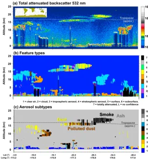
Figure 9. CALIOP observations of smoke plumes from the Australian bush fire on 15 February 2009 between 13:19 and 13:32 UTC.
(a) Total attenuated backscatter 532 nm, (b) V4 feature type classification, and (c) V4 aerosol subtypes, where the dashed line indicates the approximate location of the tropopause. The satellite ground track is indicated by the green section on the inset map in panel (a). Additional imagery for this scene, including 532 nm depolarization ratios and attenuated backscatter color ra-tios, can be found at https://www-calipso.larc.nasa.gov/products/lidar/browse_images/show_detail.php?s=production&v=V4-10&browse_ date=2009-02-15&orbit_time=12-52-14&page=3&granule_name=CAL_LID_L1-Standard-V4-10.2009-02-15T12-52-14ZN.hdf (last ac-cess: 26 September 2018).
al., 2012; Mamouri et al., 2013; Nisantzi et al., 2015), only a single value is used in the V4 algorithm. Implementing a regionally varying lidar ratio for dust is complicated due to uncertainties in determining the dust source regions for transported dust and introducing unnatural discontinuities in global dust AOD. The uncertainty in the V4 dust lidar ratio of 20 % (30 %) at 532 nm (1064 nm) accounts for the regional variability.
2.5.2 Polluted continental and elevated smoke
Polluted continental lidar ratios at 532 nm and 1064 nm are unchanged from V3 to V4, at 70±25 sr and 30±14 sr, respec-tively. For elevated smoke, the 532 nm lidar ratio is the same in both versions, but, based on a study by Liu et al. (2015), the uncertainty is reduced from 70±28 sr in V3 to 70±16 sr in V4. The lidar ratio at 1064 nm for elevated smoke is changed from 40±24 sr in V3 to 30±14 sr in V4 (Sayer
et al., 2014), so that the V4 value for smoke now matches that of polluted continental. Elevated smoke detected in the stratosphere also uses these same lidar ratios.
2.5.3 Clean continental
Cloud
(c) Aerosol subtypes after SCAARF Cloud
(b) Aerosol subtypes before SCAARF
Marine “fringes” Elevated smoke
Smoke Marine Polluted dust
Smoke Marine Polluted dust 6
4
2
0
Altitude
(km)
8
6
4
2
0
Altitude
(km)
8
6
4
2
0
Altitude
(km)
−2 −7 −12 −17
Latitude (°)
-1
sr
-1
)
Figure 10. CALIOP observations of a smoke plume off the west coast of Africa on 14 September 2008 from approximately 01:08 to
01:10 UTC.(a)Total attenuated backscatter 532 nm and aerosol subtype classification(b)before and(c)after SCAARF is implemented. The inset map in(a)shows the CALIOP ground track in red. Aerosol subtypes elevated smoke (black), clean marine (blue), and polluted dust (brown).
ratios at 1064 nm is available from Rogers et al. (2014). Con-sequently, the V4 lidar ratio for clean continental aerosol at 1064 nm remains unchanged from V3.
2.5.4 Polluted dust and dusty marine
Validation with MODIS and airborne HSRL measurements shows that CALIOP V3 AODs and lidar ratios appear to be biased high for layers in some regions which are classified as polluted dust (Kim et al., 2013; Burton et al., 2013; Rogers et al., 2014). This is especially true over the ocean. Since CALIOP V3 did not account for mixtures of dust and sea salt, which are frequent in the MBL, the bias is likely a result of dust+marine misclassified as dust+smoke. For this rea-son, the lidar ratios for polluted dust remain the same in V4 as in V3, and a new aerosol subtype, dusty marine, is intro-duced to reflect the correct mixture. The lidar ratios for pol-luted dust are unchanged from their V3 values, at 55±22 sr at 532 nm and 48±24 sr at 1064 nm. Based on an assumed external mixture of dust and marine aerosol (mixing ratio of 65:35 by surface area), the lidar ratios for dusty marine are fixed at 37±15 sr at both wavelengths, using mean lidar ratios of 44 and 23 sr for pure dust and clean marine, respectively. Using the NASA HSRL in the MBL in the Caribbean region, Rogers et al. (2014) found lidar ratios of 37±11 sr for mix-tures of dust and marine aerosols. As is the case for both dust and marine, the lidar ratios for dusty marine combination are spectrally independent. However, the lidar ratio uncertainties ascribed to the dusty marine type are larger than either dust or marine alone. The range of uncertainty of the dusty ma-rine lidar ratio in V4 (15 sr) is greater than the uncertainty for these mixtures in Rogers et al. (2014) and accounts for a
large range of possible surface area mixing ratios of dust and marine aerosols in the ambient MBL.
2.5.5 Volcanic ash
Table 3.Mean 532 nm lidar ratios reported in the literature for volcanic ash and volcanic sulfate.
Mean lidar ratio (532 nm) Volcanic eruption Reference
Ash-dominant aerosol
50±10 sr Eyjafjallajökull, 2010 Ansmann et al. (2011); Groß et al. (2012)
60±5 sr Eyjafjallajökull, 2010 Ansmann et al. (2010)
69±13 sr Puyehue-Cordón Caulle, 2011 Prata et al. (2017)
Sulfate-dominant aerosol
30–50 sr Kasatochi, 2008; Sarychev Peak, 2009 Mattis et al. (2010)
48 sr Nabro, 2011 Sawamura et al. (2012)
55 sr Mt. Etna, 2002 Pappalardo et al. (2004)
55±4 sr Sarychev Peak, 2009 O’Neill et al. (2012)
63±14 sr Sarychev Peak, 2009 Prata et al. (2017)
65±10 sr Kasatochi, 2008 Hoffmann et al. (2010)
66±19 sr Kasatochi, 2008 Prata et al. (2017)
on information gained since the 2016 release of the version 4 level 2 products.
2.5.6 Sulfate/other
Default lidar ratios for sulfate/other are 50±18 sr and 30±
14 sr at 532 and 1064 nm, respectively. Researchers have pre-viously reported independent lidar measurements of sulfate-rich volcanic plumes from the Mt. Etna 2002, Kasatochi 2008, Sarychev Peak 2009, and Nabro 2011 eruptions, sum-marized in Table 3. Lidar ratios from these studies range from 30 to 66 sr, with CALIOP-constrained lidar ratio retrievals reported by Prata et al. (2017) on the high end: 63±14 sr and 66±19 sr for the Kasatochi and Sarychev Peak erup-tions, respectively. The 532 nm lidar ratio for sulfate is con-sistent with these studies given the variability in measured lidar ratios and the 35 % uncertainty implemented with the default lidar ratio, yielding 50±18 sr. Independent measure-ments of 1064 nm lidar ratios for volcanic sulfate are sparse in the literature. The default lidar ratio value of 30 sr, how-ever, is consistent with Jäger and Hofmann (1991), who re-ported measured background stratospheric aerosol levels of 35 and 39 sr for years 1979–1980 and 1986–1987, respec-tively. The 1064 nm lidar ratio is also consistent with that of the CALIOP model for polluted continental aerosol, which is, in part, modeled after sulfate (Omar et al., 2009). 2.5.7 Polar stratospheric aerosol
Default lidar ratios for PSA are 50±20 sr at 532 nm and 25±10 sr at 1064 nm. As discussed in Sect. 2.3, these aerosol layers exhibit a qualitative spatial correlation with the STS composition class in the CALIPSO level 2 PSC mask prod-uct. These lidar ratios and their wavelength dependence are consistent with theoretical Mie scattering calculations for STS droplets at pressures typical of the Arctic stratosphere.
3 Aerosol subtyping changes from version 3 to version 4
The performance and final results delivered by the V4 aerosol subtyping algorithm are affected by V4 changes to several other algorithms that occur earlier in the level 2 processing scheme. The CALIOP V4 level 1 data significantly improved the calibration of the CALIOP attenuated backscatter coeffi-cients (β0) at both 532 and 1064 nm (Getzewich et al., 2018; Kar et al., 2018; Vaughan et al., 2018a). In particular, cali-bration coefficients at 532 nm decreased by∼3 % to∼12 %, depending on latitude and season, resulting in a concomitant increase inβ0at 532 nm. The increased magnitude ofβ0at 532 nm subsequently yields an increase in the number of ten-uous layers detected by the CALIOP feature finder. The V4 CAD algorithm features entirely new probability distribution functions (PDFs) that are now more sensitive to the presence of lofted aerosols (Liu et al., 2018). As a consequence, the V4 data products show improvements in the identification of high-altitude smoke plumes and Asian dust layers, which in earlier versions were often classified as cirrus clouds. Also, the V4 analyses use a completely new algorithm to detect the Earth’s surface detection (Vaughan et al., 2018b). This new technique demonstrates an improvement over the V3 method in turbid atmospheres, while maintaining equal or better per-formance in clear skies. As a result of this improved surface detection scheme, there are fewer opaque layers identified in V4 than there were in V3, especially at night. Because re-gions below layers previously classified as opaque are now scanned for the presence of atmospheric features, there is also a slight increase in the number of cloud and aerosol lay-ers reported. Taken together, these changes yield an increase in the absolute number of layers classified as aerosols in V4 relative to V3.
V3 changes to type j in V4; thus the summation of each column equals 100 (%). Since the total number of each type is different, relative total amounts for each type are shown as normalized total for both columns and rows, which are normalized to total number of bins for V3 aerosol.
V3 (columns) V4 (rows)
Total atten. Clear Cloud Surface Aerosol CM* Dust PC* CC* PD* Smoke Strato. feature Normalized total
Total atten. 84.30 0.03 1.42 12.98 0.09 0.13 0.06 0.06 0.01 0.11 0.02 0.00 2.09
Clear 7.14 98.97 1.92 7.81 6.28 4.43 4.99 8.88 14.87 7.10 8.61 4.11 34.18
Cloud 3.49 0.34 92.39 7.76 6.99 5.35 4.64 9.59 11.56 7.85 13.29 61.56 3.08
Surface 3.68 0.03 0.23 56.45 0.35 0.15 0.51 0.70 0.38 0.43 0.35 – 0.17
Tropo. aerosol 1.40 0.48 3.76 15.00 85.22 89.94 89.78 80.66 63.86 84.37 70.90 0.30 1.18
CM* 0.35 0.10 0.50 10.63 33.78 80.83 0.40 21.99 11.60 6.15 0.12 – 0.41
Dust 0.35 0.09 1.68 0.90 17.16 0.19 73.25 1.74 5.02 6.63 0.89 0.10 0.26
PC*/smoke 0.08 0.04 0.18 0.84 5.66 0.93 0.48 33.08 9.69 5.20 18.13 – 0.08
CC* 0.01 0.02 0.02 0.11 0.66 0.00 0.05 0.58 8.82 0.54 0.65 0.02 0.01
PD* 0.16 0.11 0.75 0.66 10.81 0.02 10.45 5.45 11.26 32.36 6.94 0.07 0.17
Elev. smoke 0.15 0.07 0.36 0.11 7.53 4.09 0.27 11.60 10.17 4.72 43.67 0.11 0.12
DM* 0.31 0.05 0.27 1.76 9.62 3.87 4.89 6.23 7.31 28.78 0.50 – 0.13
Strato. aerosol 0.00 0.16 0.27 – 1.07 0.00 0.01 0.11 9.31 0.14 6.84 34.03 0.13
PSA 0.00 0.02 0.11 – 0.06 – – 0.01 1.21 0.00 0.01 13.84 0.04
Volcanic ash 0.00 0.00 0.01 – 0.00 – 0.00 – 0.01 0.00 0.00 0.25 0.00
Sulfate/other 0.00 0.13 0.14 – 1.00 0.00 0.01 0.11 8.06 0.13 6.81 19.73 0.10
Smoke 0.00 0.00 0.01 – 0.01 – – 0.00 0.04 0.01 0.02 0.21 0.00
Total 100 100 100 100 100 100 100 100 100 100 100 100
Normalized to-tal
2.40 34.22 2.90 0.11 1.00 0.38 0.21 0.06 0.05 0.22 0.08 0.18 40.82
* CM: clean marine; PC: polluted continental; CC: clean continental; PD: polluted dust; DM: dusty marine; PSA: polar stratospheric aerosol.
V4 are analyzed using the atmospheric volume descrip-tion (AVD) reported in the level 2 aerosol profile product. AVD reports both feature type and aerosol/cloud subtype for each 5 km×60 m (5 km×180 m for above 20.2 km) range bin. The feature types include clear air, cloud, tropospheric aerosol, stratospheric feature/aerosol (V3/V4, respectively), surface, subsurface, and totally attenuated regions (i.e., be-neath layers classified as opaque in V3 but reclassified as transparent in V4). Table 4 shows changes in feature type and aerosol subtype between V3 and V4 using the AVD data in the level 2 profile products. Though the table con-tains all changes among feature types and aerosol subtypes, in this study we focus solely on changes in the distribu-tion of aerosol subtypes and the downstream effects of these changes in the global and regional distributions of AOD. 3.1 Feature type changes
Feature type changes between V3 and V4 are predominantly due to extensive changes in the calibration coefficients re-ported in the CALIOP level 1 product, which in turn required major revisions of the PDFs that drive the CAD algorithm (Liu et al., 2018). Changes to the surface detection algorithm (Vaughan et al., 2018b) also contribute, but to a significantly lesser extent. In order to quantify how the occurrence fre-quency of aerosol types has changed, Table 4 reports the
(f) Elevated smoke
(a) Clean marine (b) Dust
(c) Polluted continental / smoke
(e) Polluted dust
(d) Clean continental 60°
30°
0° −30°
−60°
60°
30°
0° −30°
−60°
60°
30°
0°
−30° −60°
−180° −120° −60° 0° 60° 120° 180° −180° −120° −60° 0° 60° 120° 180°
-40 -32 -24 -16 -8 0 8 16 24 32 40
Frequency difference (V4–V3) (%)
Figure 11.Differences in frequency of occurrence of indicated aerosol subtype from V3 to V4 (fV4 – fV3) for aerosol subtypes common to both versions, JJA 2007 day and night. Frequencies are computed from level 2 aerosol profile products and the number of aerosol samples, with the indicated aerosol type divided by the total number of aerosol samples.
3.2 Aerosol subtype changes
The spatial distribution and frequency of occurrence of aerosols has changed from V3 to V4 for reasons described in Sect. 3.1. Similarly, enhancements to the aerosol subtyp-ing algorithm described in Sect. 2 are responsible for changes in the spatial distributions and occurrence frequencies of the different aerosol subtypes. The net effect of these changes is demonstrated by Fig. 11, which shows the difference in aerosol subtype detection frequencies for JJA 2007, day and night combined. For context, Fig. 12 shows the number of aerosol samples detected during the same time period. The frequency of clean marine aerosol is slightly reduced in V4 except for in the oceans around Antarctica (Fig. 11a), with most changed layers becoming dusty marine. Table 4 shows that 3.9 % of V3 clean marine aerosol is reclassified as dusty marine in V4. The increase in clean marine aerosol in V4 over the Antarctic Ocean mainly comes from clean continen-tal and polluted continencontinen-tal aerosols due to the changes in aerosol subtyping algorithm over the polar regions (Fig. 1). Approximately 4.1 % of clean marine aerosol off the south-west African coast became elevated smoke in 2007–2009 (Table 4).
The revised definition for elevated smoke (Sect. 2.1.3) and the implementation of SCAARF (Sect. 2.3) are responsible for correcting the frequency of elevated smoke classifications in this region in V4 (Fig. 11f). Additionally, the revised ele-vated smoke definition is responsible for the changes in pol-luted continental/smoke and elevated smoke classifications over southern Africa in Fig. 11c and f, respectively. During JJA, smoke from biomass burning is ubiquitous in this re-gion, so a smoke aerosol subtype classification is expected most often. Because the top altitudes of smoke layers within this region are often below 2.5 km above the ground level, many layers do not meet the V4 elevated definition, causing an increase in the frequency of polluted continental/smoke classifications and a reduction in the frequency of elevated smoke classifications compared to V3.
Figure 12.Number of aerosol samples detected in V4 for JJA day and night combined, computed from the CALIOP level 2 aerosol profile product.
of dust has decreased (Fig. 11b), in part due to correcting the overestimate ofδpestthat existed in V3. This correction inδpest
also caused about 4.9 % of V3 dust to become dusty marine in V4 (Table 4). Though the fraction of aerosol classified as dust has changed by a small amount, the number of dust lay-ers at high altitudes has increased due to changes in CAD, which shows an improved ability to correctly classify lofted dust layers as aerosols rather than cirrus clouds (Liu et al., 2018).
The frequency of clean continental aerosol has decreased over regions characterized by snow, ice, and tundra (Fig. 11d) because all aerosol type classifications are allowed in V4 over these surface types (Sect. 2.1.1). Clean continental aerosols have mainly changed to clean marine (11.6 %), pol-luted dust (11.3 %), elevated smoke (10.2 %), and polpol-luted continental/smoke (9.7 %). The increase in dust and polluted dust classifications over the Antarctic reflect CAD misclassi-fications of tenuous ice clouds and blowing snow. Only 8.8 % of clean continental aerosol layers are unchanged in V4 (Ta-ble 4).
As a global summary, Fig. 13 shows frequency distribu-tions of aerosol subtypes for daytime and nighttime in V3 and V4, normalized by the total number of bins (day and night together for each version) that were classified as aerosol ac-cording to the AVD data from the level 2 aerosol profile prod-ucts. More aerosol layers are detected at night for both V3 and V4 (Liu et al., 2018). This is expected since a higher SNR at night means the CALIOP layer detection algorithm detects more weakly scattering features during nighttime (Vaughan et al., 2009). Clean continental is only rarely identified in V4. Clean continental was common in the polar regions, espe-cially over the Antarctic in V3. Because V4 allows all aerosol types in the poles, the dominance of clean continental is sig-nificantly reduced, as shown in Fig. 11d. The frequency of polluted dust is reduced for both day and night. While part of this reduction is due to the layer attenuation corrections
men-0 5 10 15 20
CM Dust PC CC PD Smoke DM Strato.
N
or
m
al
iz
ed
fr
eq
ue
nc
y
(%
)
Aerosol type
Figure 13.Normalized frequencies of aerosol subtypes in V3 and V4 for daytime and nighttime. Note that “strato.” represents strato-spheric features for V3 but stratostrato-spheric aerosols for V4. CM: clean marine; PC: polluted continental; CC: clean continental; PD: pol-luted dust; DM: dusty marine.
tioned in Sect. 2.1.1, the predominant reason is because lay-ers previously classified as polluted dust are now more realis-tically classified as dusty marine in V4. Since the frequency of occurrence of polluted dust aerosols is larger for daytime compared to nighttime over ocean in V3, as shown in Fig. 3b, the change from polluted dust to dusty marine is relatively more frequent for daytime than nighttime. In fact, 59 % of the daytime dusty marine in V4 is polluted dust in V3, but only 42 % of the nighttime dusty marine is polluted dust in V3. The generic stratospheric features previously identified in V3 are now classified as clouds or aerosol in V4. During the daytime, these V3 stratospheric features are more fre-quently identified as clouds, rather than aerosols. At night the situation is reversed: nighttime V3 stratospheric features are most often classified as aerosols.
3.3 AOD changes
in-Table 5.Mean column AODs (±standard deviation) for CALIOP V3 and V4, computed from aerosol extinction profiles, for all-sky conditions from 2007 to 2009. Profiles in which either V3 or V4 contained aerosol layers are included in the average.
Night Day
V3 0.084±0.162 0.090±0.150 V4 0.128±0.242 0.126±0.202
creased from 0.084 (0.090) in V3 to 0.128 (0.126) in V4 (Ta-ble 5). Day and night AOD become more compara(Ta-ble in V4, whereas daytime AOD is larger than nighttime AOD in V3. Note that the mean AOD computed here is not meant to rep-resent global conditions but instead examines AOD changes only where AOD is detected by CALIOP.
The AOD increase from V3 to V4 is due to various fac-tors. Using the feature types and aerosol subtypes reported in the level 2 AVD, AOD changes attributed to layer detec-tion, CAD, totally attenuated layers, surface detecdetec-tion, strato-spheric aerosol classification, aerosol type, and lidar ratio are identified using the procedure diagrammed in Fig. 14. This strategy isolates changes in AOD due to each of these fac-tors using CALIOP level 2 products from 2007 to 2009. All range bins whose feature type is determined as aerosol by either V3 or V4 are selected for the analyses. If a bin is iden-tified as aerosol in one of V3 or V4 and the other is clear, the corresponding AOD change is regarded as changing due to the difference of layer detection in the two versions (path-way 1 in Fig. 14). Similarly, an aerosol bin that changed from/to cloud, totally attenuated layer, surface, and strato-spheric feature is counted in the AOD changes due to the up-dates of CAD, totally attenuated signals, surface detection, and stratospheric aerosol in V4, respectively (pathways 2– 5). When feature types in both V3 and V4 are aerosol, AOD differences can be due to aerosol subtype changes (pathway 6) or lidar ratio adjustments without changing subtype (path-way 7). If aerosol subtype is identified as polluted continen-tal, polluted dust, or smoke in both V3 and V4, there are no changes in the aerosol subtyping (pathway 8). However, the AOD can be different between V3 and V4 even when there are “no changes” in their subtype and lidar ratio. The most likely source of these differences is changes in the mag-nitude ofβ0, either due to level 1 calibration improvements (Kar et al., 2018; Getzewich et al., 2018) or to changes in the two-way transmittances estimated for overlying cloud and/or aerosol layers (Young et al., 2018).
Table 6 quantifies the AOD changes from V3 to V4 for all-sky conditions for the different factors categorized in Fig. 14, i.e., layer detection, CAD, surface detection, stratospheric aerosol, aerosol subtype, lidar ratio, and no change. Here, the all-sky analysis includes all profiles that contain identi-fied aerosol regardless of the presence of clouds. All of the factors listed above contribute to the increase in AOD in V4,
and the magnitudes of the AOD changes are strongly related to their occurrence frequencies (Table 6).
Global maps of AOD changes for each factor are shown in Fig. 15. CALIOP AOD has increased by 0.007 and 0.005 for nighttime and daytime, respectively, because of changes in layer detection (Table 6 and Fig. 15b). This implies that the CALIOP V4 layer detection algorithm finds tenuous layers that were not found in V3. Note that no significant changes were made to the CALIOP layer detection algorithm in V4. The increased detection of faint layers is attributed primarily to changes in the 532 nm calibration coefficients that gener-ally increaseβ0. The CAD algorithm classifies most of these new layers as aerosols.
Figure 15c shows that AOD changes due to CAD have a day and night difference. The mean daytime AOD increase is twice the nighttime AOD increase (Table 6). The daytime AOD increase is due primarily to a net increase in the num-ber of V4 aerosols. The numnum-ber of new aerosols in V4 (i.e., layers that were classified as clouds in V3) is much larger (∼3.4 times) than the converse (i.e., the aerosols in V3 that were classified as clouds in V4) at daytime. Among these new aerosols, the subtypes dust and polluted dust account for more than 50 %. The V4 CAD PDFs were deliberately tuned to be more sensitive to aerosol presence in the upper tro-posphere and lower stratosphere, resulting in improved per-formance in distinguishing high-altitude Asian dust plumes from cirrus (Liu et al., 2018). However, as a side effect, some fraction of the cirrus fringes detected along the edges and lower boundaries of cirrus clouds that were classified as clouds in V3 are now classified as aerosols in V4. Most of these misclassified fringes are subsequently identified as dust or polluted dust by the aerosol subtyping algorithm. These increases in misclassified dust and polluted dust at high alti-tudes contribute the most to the daytime AOD increase due to CAD. Although the misclassification of cirrus fringes as aerosols also occurs in the V4 nighttime aerosol products, the gain and loss in the total aerosol number due to CAD are about the same and hence the change in nighttime aerosols cannot fully explain the increase in the nighttime mean AOD increase in Table 6. It appears that the change in V4 level 1 data calibration also plays an important role. As discussed below for Fig. 15i, changes in the V4 level 1 data calibra-tion alone can cause a nighttime AOD increase of 0.003, as shown in Table 6, about half the nighttime AOD change of 0.007 due to CAD. However, the net change for each aerosol subtype varies largely and may play an important role in the regional AOD changes as seen in the left panel of Fig. 15c.
attenu-(FT3, FT4, AT3, AT4) AT3 : aerosol subtype for V3 AT4 : aerosol subtype for V4
FT3 orFT4
= aerosol No aerosol for both V3 and V4
FT3 andFT4
= aerosol
FT3 orFT4
= cloud
AT3 = PC, PD, smoke AT3 = AT4
Layer detection
Stratospheric aerosol No changes
Lidar ratio Aerosol subtype
FT3 orFT4
= clear
CAD
FT3 orFT4
= totally
attenuated
Totally attenuated NO
YES
YES
YES
YES NO
NO
YES NO
FT3 orFT4 =
(sub)surface
Surface detection YES NO
NO
YES
YES
NO NO
8 5
7 4
6 3
1
2
Figure 14.Flowchart to categorize factors that impact the AOD change between V3 and V4. Note that changes between polluted continental and smoke are treated as no changes because the lidar ratios at 532 nm for those aerosols are the same (70 sr). FT3 and FT4 represent the feature types assigned in V3 and V4, respectively. Similarly, AT3 and AT4 designate version-specific aerosol subtypes.
Table 6.Mean column AOD changes (±standard deviation) from CALIOP V3 to V4 (defined as V4 – V3) and their bin frequencies for different reasons described in Fig. 5 for all-sky conditions from 2007 to 2009.
Frequency (%) AOD change
Night Day Night Day
Layer detection 20.9 17.5 0.007±0.050 0.005±0.061
CAD 11.7 12.2 0.007±0.159 0.014±0.121
Total attenuated 1.7 1.3 0.008±0.075 0.003±0.047
Surface detection 1.5 1.5 0.001±0.025 0.002±0.015
Stratospheric aerosol 5.5 4.0 0.001±0.020 0.002±0.017
Aerosol subtype 16.5 18.7 0.003±0.081 −0.004±0.068
Lidar ratio 31.5 36.8 0.013±0.067 0.012±0.060
No change 10.7 8.0 0.003±0.040 0.003±0.032
Total (number of samples) 100 (868, 893, 575) 100 (492, 266, 349) 0.044±0.225 0.036±0.183
ated in V3 are now searched for the presence of features, and the aerosol layers detected in these regions contribute to an increase in AOD in V4 (Fig. 15d).
Changes in the surface detection and the newly introduced stratospheric aerosol types also contribute to AOD increases in V4, but not significantly. Figure 15e shows that some sur-face signals misclassified as aerosols in V3 are now classified
Figure 15.Global maps of mean AOD differences between V3 and V4 for each factor categorized in Fig. 14 from 2007 to 2009:(a)total,
(b)layer detection,(c)CAD,(d)totally attenuated,(e)surface detection,(f)stratospheric aerosol,(g)aerosol subtype,(h)lidar ratio, and
(i)no changes. Left and right columns are for nighttime and daytime, respectively.
ubiquitous in the polar winter and are most often classified as stratospheric aerosol in V4 (Fig. 15f).
There is a decrease in the mean AOD due to aerosol subtype changes for daytime, but an increase for nighttime (Table 6). Figure 15g shows that AOD changes due to the aerosol type changes generally have opposite signs at day and night over oceans. The dominant aerosol type over oceans is clean marine, which has the smallest lidar ratio among the CALIOP aerosol models. Therefore, any changes from clean marine to other types of aerosol can lead to an AOD increase in V4. This is the dominant type change over ocean for the nighttime. For the daytime, however, a type change from polluted dust to dusty marine occurs more frequently, as explained earlier (Sect. 3.2). The reduction in lidar ratio from polluted dust (55 sr) to dusty marine (37 sr) leads to a decrease in the mean daytime AOD. AODs decrease for
both day and night over the mid-Atlantic and Indian oceans as well as over the Arctic and Antarctic oceans, as shown in Fig. 15g. Dust is frequently transported to the Atlantic and Indian oceans from the Saharan and Arabian deserts. Aerosol type changes from dust or polluted dust to dusty marine dom-inate in these regions and lead to the AOD decreases in these regions. The AOD decreases over the Arctic and Antarc-tic oceans are because the V4 aerosol subtyping algorithm now allows all aerosol types over these regions rather than solely the clean continental and polluted continental subtypes (Sect. 2.1.1).