OPTIMAL CONDUCTOR SELECTION FOR
LOSS REDUCTION IN RADIAL DISTRIBUTION
SYSTEMS USING DIFFERENTIAL EVOLUTION
Dr. R. Srinivasa Rao
Department of Electrical Engineering, J.N.T.University Kakinada, INDIA [email protected]
Abstract :
The size of conductor in a distibution system is an important parameter as it determines the current density and the resistance of the line. A lower conductor size can cause high I2R losses and high voltage drop which causes a loss of revenue as consumer’s consumption lower and hence revenue is reduced. In this paper a new approach is proposed to optimally select the conductors for minimum loss in the distribution system. Differential evolution algorithm is used to select optimal conductor type for each feeder. The objective function modeled in this paper consists of sum of capital investment and capitalized energy losscost. Voltage constraints and maximum current carrying capacity of the conductors are also incorporated in the objective function. To demonstrate the effectiveness of the proposed method, simulations are carried out on 32 bus system and results obtained are encouraging. Keywords: Optimal Conductor Selection, Loss Reduction, Radial Distribution Systems, And Differential Evolution
1. Introduction
The demand for electrical energy is ever increasing. Today over 21% (apart from theft) of the total electrical energy generated in India is lost in transmission (4-6%) and distribution (15-18%). The electrical power deficit in the country is currently about 18%. Clearly, reduction in distribution losses can reduce this deficit significantly. The main reason for having high losses in developing contries like India is stretching of distribution lines beyond the limits of load centers, increase of load abnormally without considering the current carrying capacity of the conductors and imbalance of generation and load causing reactive power generation, etc.
Hence proper selection of conductors in the distribution system is important as it determines the current density and the resistance of the line. A lower conductor size can cause high I2R losses and high voltage drop which causes a loss of revenue as consumer’s consumption lowered and hence revenue is reduced. Increasing the size of conductors will require additional investment, which may not pay back for the reduction in losses. The recommended practice is to find out whether the conductor is able to deliver the peak demand of the consumers at the correct voltages, that is, the voltage drop must remain within the allowable limits as specified in the Indian Electricity Act, 2003. The preferred solution for problems like high losses and voltage drops is network reconductoring. This scheme arises where the existing conductor is no more optimal due to rapid load growth. This is particularly relevant for the developing countries, where the annual growth rates are high and the conductor sizes are chosen to minimize the initial capital investment. Studies of several distribution feeders indicate that the losses in the first few main sections (say, 4 to 5) from the source constitute a major part of the losses in the feeder. Reinforcing these sections with conductors of optimal size can prevent these losses. Thus, we can minimize the total cost, that is, the cost of investment and the cost of energy losses over a period of 5 to 10 years. The sizing of conductor must depend upon the load it is expected to serve and other factors, such as capacity required in future.
of this method is that it cannot handle the lateral branches. Tram and Wall [3] have developed a practical computer algorithm for optimal selection of conductors of radial distribution feeders. They have also explored the possibilities of using regulator instead of reconductoring of the feeder segment to resolve the voltage problem. Wall et al. [4] have considered a few small systems to determine the best conductors for different feeder segments of these systems. Anders et al [5] analyzed the parameters that affect the economic selection of cable sizes. The authors also did a sensitivity analysis of the different parameters as to how they affect the overall economics of the system. Leppert and Allen [6] suggested that conductor selection is not only based on simple engineering considerations such as current capacity and voltage drop but also on various other considerations such as load growth and wholesale power cost increase. In this paper, the authors have proposed Differential Evolution (DE) algorithm for optimal selection of conductors in each branch of the distribution system. The algorithm is tested on 28 bus system and results are compared with other methods available in the literature.
The rest of the paper is organized as follows: Section 2 gives the problem formulation; Section 3 provides an overview of Differential Evolution; Section 4describes Solution Technique; Section 5 presents computational test results and section 6outlines conclusions.
2. Problem Formulation
2.1.Objective function
The objective of optimal conductor selection is select conductor size from the available in each branch of the system which minimizes the sum of depreciation on capital investment and cost of energy losses while maintaining the voltages at different buses within the limits. In this case the objective function with conductor c in branch i is written as
Min.imizef(i,c)CE(i,c)DCI(i,c) (1) subject to
k 2,3,...., m
for V
V(m,c) min
b 2,3,...., i
for I
I(i,c) max(c) 1, where f is sum of depreciation on capital investment and cost of energy losses of CE is the cost of Energy Losses
DCI is Depricaiation on Capital Investiment i is branch in system
c is the type of conductor used in the branch k is total number of buses in the network b is total number of branches
The annual cost of loss in branch i with conductor type k is,
} ){
,
(i c K K LSF T Loss
Peak c) (i,
CE P E (2)
where Kp is Annual demand cost due to power loss (Rs/kW), Ke is Annual cost due to energy loss(Rs/kWh) LSF is Loss factor
Peak loss(i,c) is Real power loss of branch i under peak load conditions with conductor type c T is the time period in hours (8760 hours)
Depreciation on capital investment (DCI) is given as
)} ( ) ( { * ) (
*Ac Cost c leni IDFC
c) (i,
DCI (3)
where IDFC is Interest and depreciation factor Cost (c) is Cost of c type conductor (Rs /km) Len (i) is Length of branch i (km)
A(c) Cross-Sectional area of c type conductor in mm2
Loss factor is defined as ratio of energy loss in the system during a given time period to the energy loss that could result if the system peak loss had persisted throughout that period. In British experience, loss factor is expressed in terms of the load factor (Lf) as
Lf Lf
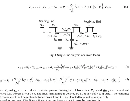
Sending End Receiving End
Vk Vk+1
V0 Vn
Yk1 Yk2 Pk + jQk rk + jxk ' k k jQ P 1 k 1 k jQ
P PnjQn
1
1
Lk Lk jQ
P V0
2.2.. Evaluation of fitness function
The evaluation of fitness function is a procedure to determine the fitness of each string in the population. Since the DE proceeds in the direction of evolving best-fit strings and the fitness value is the only information available to the DE, the performance of the algorithm is highly sensitive to the fitness values. The fitness function F, which has been chosen in this problem, is
c) f(i, F 1 1 (4)
2.3. Power Flow Analysis
The power flows are computed by the following set of simplified recursive equations [5] derived from the single-line diagram shown in Fig. 1.
1 , 1
( 2)2
Lk1k k k 2 k 2 k k k Lk k Loss k
k P Q Y V P
V r P P P P
P (5)
Fig. 1 Single-line diagram of a main feeder
11 ,
1 ( )
Lk
2 1 k 2 k 2 k 1 k 2 2 k 1 k k 2 k 2 k k k Lk k Loss k
k P Q Y V Y V Y V Q
V x Q Q Q Q
Q (6)
'
'
( )
( )
1 2 k k k k k k 2 2 k k k 2 k 2 k 2 k 2 k 2 k k k k k 2 k 2 k 2 k 2 k 2 k 2 k 2k P Q Y V 2rP x Q Y V
V x r V Q x P r 2 Q P V x r V
V (7)
where Pk and Qk are the real and reactive powers flowing out of bus k, and PLk+1 and QLk+1 are the real and reactive load powers at bus k+1. The shunt admittance is denoted by Ykl at any bus k to ground. The resistance and reactance of the line section between buses k and k+1 are denoted by rk and xk, respectively.
The peak power loss of the line section connecting buses k and k+1 may be computed as 2 2 ' 2 ) ( . ) 1 , ( k k k k Loss Peak V Q P r k k
P (8)
The total power loss of the feeder, PT,Peak Loss, may then be determined by summing up the losses of all line sections of the feeder, which is given as
b k Loss Peak ss o L PeakT P k k
P
1
, ( , 1) (9)
3. Overview of Differential Evolution
One extremely powerful algorithm from convergence characteristics and few control parameters is differential evolution. Differential evolution solves real valued problems based on the principles of natural evolution [6] using a
population P of Np floating point-encoded individuals that evolve over G generations to reach an optimal solution. In differential Evolution, the population size remains constant throughout the optimization process. Each individual or candidate solution is a vector that contains as many parameters as the problem decision variables D. The basic strategy employs the difference of two randomly selected parameter vectors as the source of random variations for a third parameter vector. In the following, we present a more rigorous description of this new optimization method.
]
[ 1 G
Np G
X , ... , X
P (10)
Np , ... 1,2, i , X ... X X
XiG [ 1G,i 2G,i DG,i]T (11) Extracting distance and direction information from the population to generate random deviations result in an adaptive scheme with excellent convergence properties. Differential Evolution creates new offsprings by generating a noisy replica of each individual of the population. The individual that performs better from the parent vector (target) and replica (trail vector) advances to the next generation. This optimization process is carried out with three basic operations:
Mutation Cross over Selection
First, the mutation operation creates mutant vectors by perturbing each target vector with the weighted difference of the two other individuals selected randomly. Then, the cross over operation generates trail vectors by mixing the parameters of the mutant vectors with the target vectors, according to a selected probability distribution. Finally, the selection operator forms the next generation population by selecting between the trial vector and the corresponding target vectors those that fit better the objective function.
3.1. DE Algorithm
Initialize population
While stopping criteria are not satisfied,
o Create mutant vector with the difference vector and scaling constant o Generate trial vectors applying the selected crossover scheme
o Select next generation members according to competition performance.
3.2.DE Optimization Process
3.2.1. Initialization
The first step in the DE optimization process is to create an initial population of candidate solutions by assigning random values to each decision parameter of each individual of the population. Such values must lie inside the feasible bounds of the decision variable and can be generated by (12). In case a preliminary solution is available, adding normally distributed random deviations to the nominal solution often generates the initial population.
D ., 1,2,... j
Np; , ... 1,2, i X
X X
X j j j j
0 i
j ( )
min max min
) (
, (12)
where i=1,2,....Np and j=1,2,...,D; min j
X and Xmaxj are respectively, the lower and upper bound of the j th decision parameter and j is a uniformly distributed random number within [0,1] generated anew for each value of j. X(j0,i)is the jth parameter of the ith individual of the initial population.
3.2.2. Mutation
Np , ... 1,2, i X X S X
Xi'G aG ( bG CG) (13) where Xa, Xb, Xc are randomly chosen vectors{1,2, ... ,Np}and abci; Xa ,Xb ,Xc are generated anew for each parent vector; The scaling constant (F) is an algorithm control parameter used to control the perturbation size in the mutation operator and improve where algorithm convergence.
3.2.3. Crossover
The crossover operator creates the trial vectors, which are used in the selection process. A trail vector is a combination of a mutant vector and a parent (target) vector based on different distributions like uniform distribution, binomial distribution, exponential distribution is generated in the range [0, 1] and compared against a user defined constant referred to as the crossover constant. If the value of the random number is less or equal than the value of the crossover constant, the parameter will come from the mutant vector, otherwise the parameter comes from the parent vector.
The crossover operation maintains diversity in the population, preventing local minima convergence. The crossover constant (CR) must be in the range of [0, 1]. A crossover constant of one means the trial vector will be composed entirely of mutant vector parameters. A crossover constant near zero results in more probability of having parameters from the target vector in the trial vector. A randomly chosen parameter from the mutant vector is always selected to ensure that the trail vector gets at least one parameter from the mutant vector even if the crossover constant is set to zero.
otherwise X q j or CR if X X G j i j G j i G j i , ' ' , '' ,
(14)
where i = 1, 2, … , Np; j = 1, 2, …, D; q is a randomly chosen index {1,2, ... ,Np}that guarantees that the trial vector gets at least one parameter from the mutant vector; 'j
is a uniformly distributed random number within [0, 1) generated anew for each value of j. G
j i X, ,XiGj
'
, and XiGj ''
, are the jth parameter of the ith target vector, mutant vector and trial vector at generation G, respectively.
3.2.4. Selection
The selection operator chooses the vectors that are going to compose the population in the next generation. This operator compares the fitness of the trial vector and fitness of the corresponding target vector, and selects the one that performs better.
Np 1,2,..., i otherwise X X f f(X for X X G i G i G i G i G i
1 '' '' ) ( ) (15)
This optimization process is repeated for several generations allowing individuals to improve their fitness as they explore the solution space in the search for optimal values. DE has three essential control parameters: Scaling factor (S), Cross over constant (CR) and population size Np. The scaling factor is a value in the range (0,2] that controls the perturbation in the mutation process. Cross over constant is a value in the range of [0,1] that controls the diversity of the population. Population size determines the number of individuals in the population and provides tha algorithm enough diversity to search the solution space.
4. Differential Evolution Solution Technique
In the optimal conductor selection problem, the elements of the solution consist of all the control variables, i,e., all elements of the branches. These variables are represented continuous variables in the DE population.
Parameters Selection: In the process of optimization using DE, the numbers of branches are selected as
parameters. These parameters are encoded using suitable techniques. There are various encoding techniques are available, because of simplicity binary encoding technique is chosen for encoding and decoding. In this problem, only one parameter is encoded that is conductor size. For each branch, string length is taken as 2.Therefore total length of the string is two times that of the total number of branches in the network.
Population Size and Initialization of Population: The size of population i.e., no. of chromosomes in a
population, is direct indication of effective representation of whole search space in one population. The population size affects both the ultimate performance and efficiency of DE. In this problem, a population size of 10 is chosen. The population is initialized with 1’s and 0’s randomly, so that they can have wide search space.
Chromosome String Representation: Before applying a DE to any task, a computer compatible representation
No Start Read the system data
Perform Load Flow Analysis, find the bus voltages & power losses and Evaluate the
objective and fitness functions
Generate new population and apply DE operators Reproduction, Cross Over and Mutation
Constraint voilation ?
Last Chromosome?
Stop i=i+1
No
Yes
Yes
Set iteration count, i=1
1. Read the conductor data and Initialize the population randomly
2. Perform load flow analysis, Evaluate the objective function (Power Loss) and fitness
function for the selected population
Store best fitness value Fitness value
improved? No
Take next Chromosome
No
Yes
i ≤ Imax
Output the best result
Fig. 2. Flow chart of the proposed method
Encoding and Decoding: Implementation of a problem in a DE starts from the parameter encoding (i.e., the
representation of the problem). The encoding must be carefully designed to utilize the DE's ability to efficiently transfer information between chromosome strings and objective function of problem. The proposed approach uses the string length that represents the conductor size in each branch of the system. Two bits are reserved for each branch. The encoding scheme of the string size is as shown.
D0 D1 D2 D3 ... D(i-1) Di
X0 X1 X0 X1 X0 X1
where Di(0,1),i1,2,......,SL(String length)
Evaluation of a chromosome is accomplished by decoding the encoded chromosome string and computing the chromosome's fitness value using the decoded parameter. The decoding of string can be expressed as:
b i
N ., 1,2,... j
and 2; 1to i , Di j
Encod[ ]
( 2 ) where Nb is number of branches.
Evaluation of Fitness Function: The evaluation is a procedure to determine the fitness of each string in the
population and is very much application oriented. Since the DE proceeds in the direction of evolving better fit strings and the fitness value is the only information available to the DE, the performance of the algorithm is highly sensitive to the fitness values. In case of optimization problems the fitness is the value of the objective function to be optimized. The fitness function which has chosen in this problem is
c) f(i, F
1 1
Crossover: Uniform crossover technique is adapted in this problem. For carrying out the crossover, there is a
need to identify the parents. The parent selection is done by using the Roulette wheel technique. This parent selection is to be repeated two times to get the two parents for crossover. After selecting the parents, a random number is generated between 0 and 1, and then this random number is compared with the crossover probability (Pc). If it is less than Pc, crossover is performed. If it is greater than Pc, Par1 and Par2 are directly selected as Chld1 and Chld2. The crossover probability is taken as 0.80.
Mutation: Mutation is the process of random modification of the value of a string position with a small
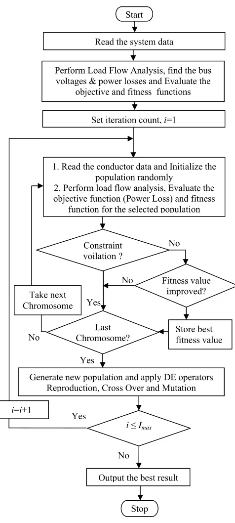
probability. It is not a primary operator but it ensures that the probability of searching any region in the problem space is never zero and prevents complete loss of genetic material through reproduction and crossover. The mutation probability is taken as 0.03. The main computational steps of the proposed method for optimal selection of conductors are given in the flowchart as shown in fig. 2.
5. Test Results
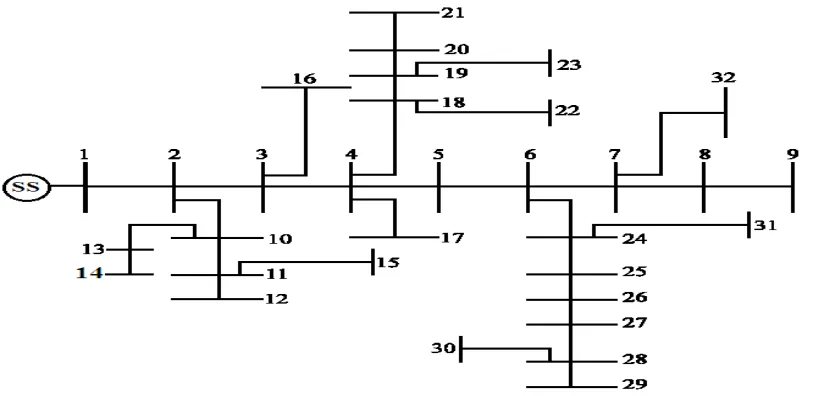
The effectiveness of the proposed algorithm has been tested on a 32-bus radial distribution systems. The single line diagram [9] for practical 32-node radial distribution systems is shown in Fig.3. The rated voltage of the network is 11 kV. The substation voltage (bus 0) is taken as 1 p.u. The line and load data are given in Appendix A. The properties of the conductors used in the analysis of this system is given in Table 1. The parameters used in this algorithm are: Number of iterations is 50; Population size is 20; Cross over probability is 0.8; and Mutation probability is 0.03. The other parameters used in compuation process are: KP= Rs. 2500/kW; KE= Rs. 0.5/kWh; LSF=0.2; and IDFC=0.1. The proposed algorithm is applied to this system and the results of conductor type selection are presented in Table 2 From Table 2. From the results, it is observed that reconductoring is necessary for all the branches except for 22 and 23.
Fig. 3. Single line diagram for 32-bus radial distribution system
after conductor grading in each brach is given in the Table 2. The minimum voltage is improved from 0.9078 p.u to 0.9205 p.u. The improvement in voltage regulation is 2%. The voltages before and after conductor grading in each brach is also presented in the Table 2. Annual cost of power loss in all branches before conductor grading is Rs. 392334.92 and after conductor grading is Rs. 326269.76. Total reduction in annual cost of power loss is Rs. 6665.2 which is approximately 16.84% of total cost of power loss. Depreciation on capital investment cost before conductor grading is Rs. 66891.69 and after grading is Rs. 52401.10.
Table 1. Conductor Types And Their Data
Table 2. Test Results of 32-Bus System
Item Before conductor
grading Method in [8]After conductor grading Proposed Method
Conductors used`` 1-21: Rabit 1- 31:Mink 1-10: Mink; 11-20: Ferret;
21-31: Weasel 21-23: Weasel; 24-31: Squirrel
Min. Voltage (p.u) (bus 25) 0.9078 0.9127 0.9205
Peak Power Loss (kW) 117.49 101.67 96.64
Loss Reduction (%) -- 13.46 17.75
(1) Power loss (Rs.) 392334.92 340155.54 326269.76
(2) Depreciation cost (Rs.) 6665.2 5789.25 52401.1
Total Cost (Rs.) [(1)+(2)] 459226.5 398024.79 378670.9
Reduction in total cost (%) -- 13.33 17.54
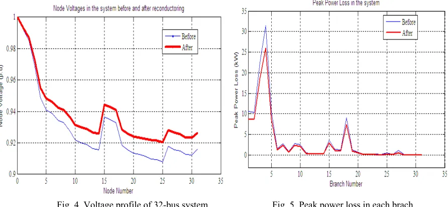
Total reduction in Depreciation on capital investment cost is Rs. 144905.59 which is approximately 21.66% of Depreciation on capital investment cost. Total cost (sum of annual cost of power loss and Depreciation on capital investment cost) before conductor grading is Rs. 459226.5 and after grading is Rs. 378670.9. The reduction in the cost is Rs. 80555.6, which is 17.54 % of total cost. The voltage profile in the system before and after conductor grading is depicted in fig. 4.
Fig. 4. Voltage profile of 32-bus system
Fig. 5. Peak power loss in each brach
From Fig. 4, it is observed that voltage at each bus improved. The peak power loss in each branch of the system before and after conductor grading is depicted in fig. 5. The power loss in the branches are reduced and thus
Type of
Conductor A (mm
2) R
ohm/km ohm/km X I(A) MAX (Rs/Km) Cost Squirrel 12.90 1.3740 0.3915 115 1260
Weasel 19. 35 0.9116 0.3820 150 1420
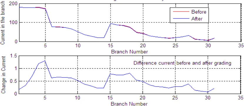
reducing the thermal loading on the conductors. Further the system is available to carry more power. The current in each branch and change in the current in each branch before and after conductor grading is shown in fig.6. From the figure, it is observed that the current through each branch is reduced after conductor grading. The results of the proposed method is compared with the results of the method proposed in [8] and presented in Table II. As per the method in [8], all conductors in the branches of the system is replaced with ‘Mink’ type conductors after grading. With the proposed method, reconductoring is done for all branches except 22 and 23. The peak power loss and total cost reduction by the proposed method is less than that of the method proposed in [8].
Fig. 6. Current profile in the system before and after conductor gading
6. Conclusions
In this paper, differential evolution algorithm has been applied to solve the optimal conductor grading problem in distribution system. The proposed algorithm is tested on 32-bus system and results obtained are encouraging. Grading of conductors are done for all branches of the system except to 22 and 23 branches. Total peak power loss before conductor grading is 117.49 kW and after conductor grading is 96.64 kW. The reduction in peak real power loss is 20.85 kW which is approximately 17.75% of the total. The voltage regulation in the system is improved by 2%. Annual cost of power loss in all branches before conductor grading is Rs. 392334.92 and after conductor grading is Rs. 326269.76. Total reduction in annual cost of power loss is Rs. 6665.2 which is approximately 16.84% of total cost of power loss. Depreciation on capital investment cost before conductor grading is Rs. 66891.69 and after grading is Rs. 52401.10. Total reduction in Depreciation on capital investment cost is Rs. 144905.59 which is approximately 21.66% of Depreciation on capital investment cost. Total cost (sum of annual cost of power loss and Depreciation on capital investment cost) before conductor grading is Rs. 459226.5 and after grading is Rs. 378670.9. The reduction in the cost is Rs. 80555.6, which is 17.54 % of total cost. Results of the proposed method is compared with the results of the other method and presented in Table 2. The results show that the performance of the proposed method is better than the other method.
Appendix A
Line And Load Data Of 32-Bus System
Branch Number Sending End Receiving End Type of Conductor Length (kM) kVA (pf=0.8)
1 1 2 Rabbit 0.20 100.00
2 2 3 Rabbit 0.20 100.00
3 3 4 Rabbit 0.43 100.00
4 4 5 Rabbit 0.60 300.00
5 5 6 Rabbit 0.22 0.00
6 6 7 Rabbit 0.16 63.00
8 8 9 Rabbit 0.10 250.00
9 9 10 Rabbit 0.40 500.00
10 10 11 Rabbit 0.60 500.00
11 11 12 Rabbit 0.24 250.00
12 12 13 Rabbit 0.24 250.00
13 13 14 Rabbit 0.60 0.00
14 14 15 Rabbit 0.50 350.00
15 6 16 Rabbit 0.25 250.00
16 16 17 Rabbit 0.11 100.00
17 17 18 Rabbit 0.11 350.00
18 18 19 Rabbit 1.00 63.00
19 19 20 Rabbit 0.32 0.00
20 20 21 Rabbit 0.25 250.00
21 21 22 Rabbit 0.10 0.00
22 22 23 Weasel 0.20 100.00
23 23 24 Weasel 0.30 100.00
24 24 25 Weasel 0.10 200.00
25 25 26 Weasel 0.50 350.00
26 19 27 Weasel 0.10 250.00
27 27 28 Weasel 0.43 550.00
28 20 29 Weasel 0.25 200.00
29 22 30 Weasel 0.10 250.00
30 30 31 Weasel 0.15 100.00
31 14 32 Weasel 0.20 313.00
References
[1] Funk Houser A.W.; 1955. A method for determining ACSR conductor sizes for the distribution systems, AIEE Trans. on PAS, pp. 479-484.
[2] Ponnavaiko M. and Rao K.S.P.; 1982. Anapproach to optimal distribution system planning through conductor grading, IEEE Trans on PAS, vol. PAS-101, pp.1735-1742.
[3] Tram H.N. and Wall D.L.; 1988. Optimal Conductor selection in planning radial distribution systems, IEEE Trans. on Power Systems, vol.3, No.1, pp. 200-206.
[4] D. Wall, G. Thompson, J. Green.; 1979. An optimization model for planning radial distribution network” IEEE Trans. on Power Apparatus and Systems, vol. 98, pp. 1061-1065.
[5] Smarajit Ghosh and Karma Sonam Sherpa.; 2008. An Efficient method for Load-Flow Solution of Radial Distribution Networks, International Journal of Electrical Power and Energy Systems Engineering, vol. 1, no. 2, pp. 108-115.
[6] K. Price, R. Storn, and J. Lampinen.; 2005. Differential Evolution: A Practical Approach to Global Optimization, Natural Computing Series, Springer-Verlag.
[7] R Gnanadass, P Venkatesh, T G Palanivelu, K Manivannan; 2004. Evolutionary Programming Solution Of Economic Load Dispatch With Combined Cycle Co-Generation Effect, Institute Of Engineers Journal-EL, vol. 85, pp. 124-128.