PERFORMANCE OF SINGLE
MODULAR MANUFACTURING UNIT
WITH QUEING MODEL BASED
MATERIAL HANDLING SYSTEM
USING AGVS
C. J. Rao 1, D. Nageswara Rao 2, and V. Sai Srikanth 3
1. Professor, Dept. of Mechanical Engineering, Aditya Institute of Technology and Management, K.Kotturu, Tekkali-532 201, Srikakulam (Dist.), Andhra Pradesh, India 2. Professor, Dept. of Mechanical Engineering., Andhra University College of Engineering (Autonomous), Visakhapatnam, Andhra Pradesh,
India
3. Associate Professor, Dept. of Mechanical Engineering, College of Engineering, GITAM University, Visakhapatnam, Andhra Pradesh, India.
ABSTRACT
Manufacturers throughout the world are facing new demands like greater product variety, shorter product life cycles, lower unit costs and higher product quality. To respond to variation in style, quantities, and quick responses, manufacturers are beginning to experiment with new manufacturing concepts. One of the most popular concepts is Modular Manufacturing. This paper concerns the study of a relatively simple manufacturing module consisting of various machines depending upon the product to be made. Since the system is modular, it is easier to construct models quickly with a variety of alternate configurations. Modular manufacturing requires a versatile means of moving parts and components from one point to another within the production process which is performed by an Automated Guided Vehicle System (AGVS). Experiments are conducted to evaluate the efficiency and other parameters practically. An attempt is made to balance the system and predict its throughput using an analytic model. Then the system is simulated in detail using Show Flow Simulation and compared with experimental results.
Key words: Modular manufacturing, Module, Automated Guided Vehicles, Modularity
1. INTRODUCTION
The parts, products and manufacturing equipment as well as the design and operating activities themselves are all described in units called modules [6], [7]. A manufacturing system is constructed and operated by combining these building blocks. Hardware and software modules are combined to meet specific requirements [3]. Modular manufacturing uses a team-based production cell or module of 5 to 10 operators that completes an entire product before starting the next. It requires operators to use a number of machines and to work with the team to plan and complete the production of each product [2], [20].
In a manufacturing system, raw materials are converted into finished products by a set of processing steps. Because the processing capability of a typical resource is limited, multiple processing operations are required. So, a transport system is employed to deliver materials between resources (machines). This transport system is expected to provide sufficient performance without limiting the system throughput or causing excessive work-in-process. This is an extremely critical function in most manufacturing systems. In simple terms, the function of material handling is the movement of material from one point to another. There is a large variety of material handling devices which have been developed to support this function. These devices are frequently categorized into the following equipment classes:
1. Industrial Trucks: hand or powered vehicles used to intermittently move items across a fixed surface. Common examples are forklift trucks, hand carts, and automated guided vehicles (AGV).
2. Cranes, Hoists: mechanical devices used to intermittently move items through space. Common examples are overhead cranes, industrial robots, and hoists.
3. Conveyors: powered devices used to move items continuously and simultaneously along a fixed path. Common examples are belt conveyors and trolley conveyors.
Automated Guided Vehicles Systems (AGVS) are among various advanced material handling techniques that are finding increasing applications in today's advanced manufacturing settings [10]. An AGV is a driverless, battery-poweredvehicle with programmable capabilities for guidance and steering. AGVs are capable of transporting a variety of part types from point to point without human intervention. They can be interfaced to various other production and storage equipment and controlled through an intelligent computer control system [11]. This flexibility and compatibility make an AGV a feasible alternative to traditional material handling methods especially in modular manufacturing environment [5]. An AGV accomplishes a delivery by a sequence of asynchronous movements [9]. However, designing an AGVS is a complex task [8]. The interaction of the AGVS with the production system must be considered [16].
Figure: 1-2 Photograph showing constructional Details of AGV
This paper focuses on the performance analysis of modular manufacturing with single AGV for transportation of raw material, work in process and finished products. Figures 1-1 and 1-2 show details of AGV with no steering mechanism. In case studies taken up here, single modules of manufacturing units with to-and-fro motion AGVs are constructed. The results obtained in this paper make a process designer familiar with the modular manufacturing in terms of its flexibility and mass customization capability. The remainder of the paper is organized as follows. Methodology followed is explained in section2.Section 3presents experimental set up with single module connected by single to-and-fro motion AGV. Section 4 describes how simulation of the same set up is run on Show Flow simulation. Results are analyzed in section 5 and the paper is concluded in section 6.
2. METHODOLOGY
Modular Manufacturing has been recognized as one of the recent technological advances which make use of basic concepts of cellular manufacturing. Modular manufacturing involves not only reduce cost of production but also involves production of more product variety with less time and effort. For simplicity one module arrangement of machines for producing four components is considered. Data of production processes are noted down and analyzed for any changes required in regard to balance the production flow. Before that, process times were established by conducting each operation six times and taking average of these six time durations. The same arrangement is tested in simulation software ShowFlow to ascertain the data generated in all the cases.
2.1 SHOW FLOW
Show Flow is software product designed to model, simulate, animate and analyze process in logistics, manufacturing and material handling. The software will shows the throughput of a production system, identify bottlenecks, measures lead-times and report utilization of resources.
Show Flow can be used to support investment decisions, to verify designs of manufacturing systems, to experiment with different manufacturing strategies or to test the performance of proposed material handling installations. Show Flow offers a wide range of features for modelling, simulation, statistics, analysis, animation and documentation.
2.1.1 HOW TO MODEL
The software includes Modelling elements like Queue, buffer, wait space, parking, machine, operations, task, resources, Transport, vehicle, car, truck, AGV, conveyor, etc.
Modelling deals with:
Element specific parameters:
1. Queue: order LIFO,FIFO, ascending/descending by attribute value 2. Conveyor : speed, length, spacing, curve, accumulation
3. Transport: speed, acceleration, deceleration, lift speed 4. Path: maximum, allowed speed, curve, directions. 5. Warehouse: rows, columns, cell size, locations. 6. Reservoir: accept control levels. release control levels
Simulation: Show Flow adopts the Optimized Simulation Algorithm Technique (OSAT) fixed time simulation runs, variable time simulation runs.
Statistics: Probability functions, constant, uniform, normal, negative exponential, lognormal, Erlanger, Empirical (user defined), gamma, triangular, beta etc.
Analysis:
Input data analysis: Dataset analysis, derive average and standard deviation, best fit suggestion, graphical display of density functions, graphical display of distribution samples.
Output data analysis: Queue graphs (queue length in time), queue histograms, wait time histograms, utilization pies, element statistics diagrams, dynamic request display, and user defined graphs, trace reports etc.
Experimentation: warm-up period determination (welsh), sensitivity analysis, automatic simulation of alternatives etc.
Animation: It includes 2D full animation, 2D statistics animation, 3D wire animation, 3D solid animation, camera position, zoom, rotate, wide angle etc.
Documentation: automatic model documentation, sorted by functionality, sorted by element, simulation event trace reports, and elements reports; input parameter value listing, etc.
3. EXPERIMENTAL SET-UP
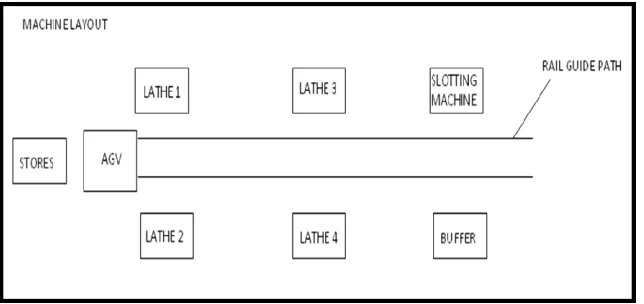
A single module with various machines (Figure: 3-1) arranged according to the requirement of the job to be produced. In this experiment four components are produced separately with their respective modular arrangement with single AGV serving for the movement of material between machines, store and buffer. The AGV utilisation depends on the material handling, layout and type of production. Here we calculated the utilisation of AGV.
We determined the travelling time and job details for various jobs (lathe job, square bolt, etc.) in a single line layout using an AGV model. All values are tabulated. Experimental results are compared with that of ShowFlow simulation
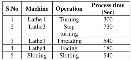
3.1 HEXAGONAL BOLT
Figure 3-1. Hexagonal bolt Table 3-1. Hexagonal bolt operations timings
S.No Machine Operation Process time (Sec)
1 Lathe 1 Turning 300
2 Lathe2 Step turning
720 3 Lathe3 Threading 540
4 Lathe4 Facing 180
Figure 3-2. Machine layout
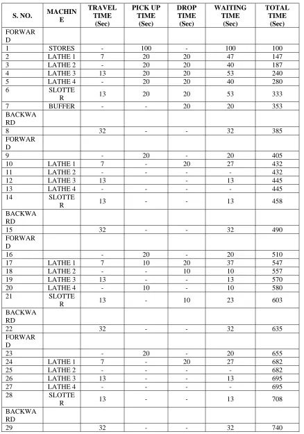
Table 3-2. Hexagonal bolt timings
S. NO. MACHIN E
TRAVEL TIME
(Sec)
PICK UP TIME
(Sec)
DROP TIME (Sec)
WAITING TIME
(Sec)
TOTAL TIME
(Sec)
FORWAR D
1 STORES - 100 - 100 100
2 LATHE 1 7 20 20 47 147
3 LATHE 2 - 20 20 40 187
4 LATHE 3 13 20 20 53 240
5 LATHE 4 - 20 20 40 280
6 SLOTTE
R 13 20 20 53 333
7 BUFFER - - 20 20 353
BACKWA RD
8 32 - - 32 385
FORWAR D
9 - 20 - 20 405
10 LATHE 1 7 - 20 27 432
11 LATHE 2 - - - - 432
12 LATHE 3 13 - 13 445
13 LATHE 4 - - - - 445
14 SLOTTE
R 13 - - 13 458
BACKWA RD
15 32 - - 32 490
FORWAR D
16 - 20 - 20 510
17 LATHE 1 7 10 20 37 547
18 LATHE 2 - - 10 10 557
19 LATHE 3 13 - - 13 570
20 LATHE 4 - 10 - 10 580
21 SLOTTE
R 13 - 10 23 603
BACKWA RD
22 32 - - 32 635
FORWAR D
23 - 20 - 20 655
24 LATHE 1 7 - 20 27 682
25 LATHE 2 - - - - 682
26 LATHE 3 13 - - 13 695
27 LATHE 4 - - - - 695
28 SLOTTE
R 13 - - 13 708
BACKWA RD
Three more jobs hexagonal nut (Figure: 3-3), lathe job (job is so named as all the operations are of lathe) (Figure: 3-5) and square bolt (Figure: 3-7) are completed with respective modular layouts (Figure: 3-4), (Figure: 3-6) and (Figure: 3-8). As is done for hexagonal bolt, job reports are done for these three jobs also (tables not shown). From these status reports and job reports the performance is analyzed.
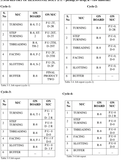
3.1.1 JOB REPORT OF HEXAGONAL BOLT (P.U – pickup, D- drop, R – raw material).
Cycle-1: Cycle-2:
S.
No M/C
ON
BOARD ON M/C
1 TURNING R-8, T-2 P.U-2T, D-2R 2 STEP
TURNING
R-8, ST-2
P.U-2ST, D-2T 3 THREADING R-8,
TH-2
P.U-2TH, D-2ST 4 FACING R-8, F-2 P.U-2F,
D-2TH 5 SLOTTING R-8, S-2 P.U-2S,
D-2F
6 BUFFER R-8
FINAL PRODUCT
TWO
Table 3-3. Job report (cycle-1)
Table 3-4. Job report (cycle-2) S.
No M/C
ON BOARD
ON M/C
1 TURNING R-8 P.U-0, D-2R 2 STEP
TURNING R-8
P.U-0, D-0 3 THREADING R-8 P.U-0,
D-0 4 FACING R-8 P.U-0,
D-0 5 SLOTTING R-8 P.U-0,
D-0
6 BUFFER -- --
S.
No M/C
ON BOARD ON M/C 1 TURNING R-8, T-1 P.U- 1 T D- 2 R 2 STEP
TURNING R-8 P.U-0 D -2 R 3 THREADING
R-8 P.U- 0 D-0 4 FACING
R-8, F-1 P.U-1 F D-0 5 SLOTTING R-8 P.U- 0
D- 1 F
6 BUFFER -- --
Cycle-3:
Table 3-5 Job report
Cycle-4:
S.
No M/C
ON BOARD
ON M/C
1 TURNING
R-8 P.U-0 D-2 R 2 STEP
TURNING R-8 P.U-0 D-0 3 THREADING R-8 P.U-0
D-0 4 FACING
R-8 P.U-0 D-0 5 SLOTTING
R-8 P.U-0 D-0 6 BUFFER
_ _
3.2 HEXAGONAL NUT
Figure 3-3. Hexagonal nut Table 3-7. Hexagonal nut process times
Figure3-4. Machine layout for hexagonal nut
3.3 LATHE JOB
Figure3.5 Lathe job Table 3-13 Lathe job process times S.N
o
Machine Operation Process time(sec
)
1 SLOTTI NG
SLOTTIN G
600 2 DRILLI
NG
DRILLIN G
120 3 TAPPIN
G
THREADI NG
300
S.No Machin e
Operatio n
Process time(se
c)
1 Lathe 1 FACING 180
2 Lathe2 TURNIN
G 300
3 Lathe3 GROOVI
NG 180
4 Lathe4 TAPER
TURNIN G
600 5 Lathe5 KNURLI
Figure 3-6. Machine layout
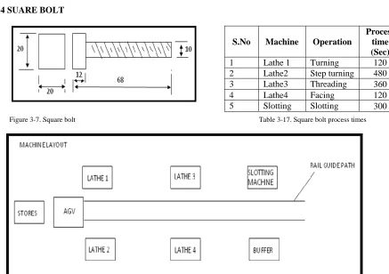
3.4 SUARE BOLT
Figure 3-7. Square bolt Table 3-17. Square bolt process times
Figure 3-8 Machine layout for square bolt
4. SHOW FLOW SIMULATION
There are three fundamental entities in ShowFlow that we use to make a model. They are Elements,
Products and Clusters. There are nine different kinds of elements, the three most important are: Machines, Buffers and InOuts. The properties of an element are divided into three categories: the element parameters, the job parameters and the stage parameters. The properties which are related to the physical part of the element are categorised in the element parameters, such as the capacity, the failure rate etc. On an element an operation (on a product) can take place. The items related to an operation are called the job parameters,
S.No Machine Operation
Process time (Sec)
1 Lathe 1 Turning 120
2 Lathe2 Step turning 480 3 Lathe3 Threading 360
4 Lathe4 Facing 120
like cycle time, batch size, etc. The definition of the routing of products through the model is done with the stage parameters of an element.
4.1 Execution of Simulation:
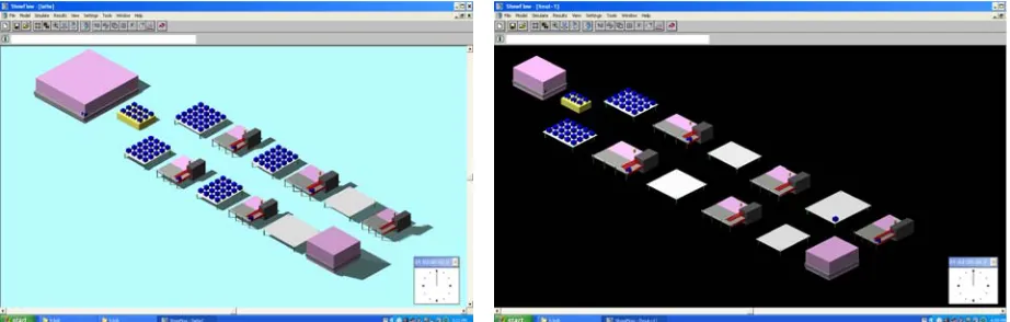
Module layouts for each set-up are generated. Simulation carried out for 10 hours cycle time for each manufacturing set-up. The results are generated from which various performance curves are plotted. Animated material flow and carrier’s movement shows the accumulation of Work In Process (WIP). Each movement can be recorded and for each movement, time duration can be noted. For each type of product, after each simulation various parameters are stored (i.e., generated) which are extracted for further analysis. Following diagrams are of layout windows generated by ShowFlow simulation for each type of product.
Figure4-1. Hexagonal Bolt simulation window Figure4-2. Hexagonal Nut simulation window
5. SIMULATION RESULTS AND GRAPHS:
HEXAGONAL BOLT REPORT
0 20 40 60
0 5 10 15
JOB NUMBER A VER AGE QUEU E SIM1 SIM2 SIM3
Figure:5‐1
HEXAGONAL BOLT REPORT
0 0.5 1 1.5
0 5 10 15
JOB NUMBER AV G W A ITI N G TI M E ( 1 0 4 ) SIM1 SIM2 SIM3
Figure: 5‐2
HEXAGONAL NUT REPORT
0 20 40 60
0 2 4 6 8 10
JOB NUMBER AV ER A G E Q U EU E SIM1 SIM2 SIM3
Figure: 5‐3
HEXAGONAL NUT REPORT
0 0.5 1 1.5 2
0 5 10
JOB NUMBER A V G W A IT IN G T IME (1 0 4 ) SIM1 SIM2 SIM3
Figure: 5‐4
LATHE JOB REPORT
0 20 40 60
0 5 10 15
JOB NUMBER AV ERA G E QUE U E SIM1 SIM2 SIM3
Figure: 5‐5
LATHE JOB REPORT
0 5 10 15
0 5 10 15
JOB NUMBER AVG W A IT IN G TI M E ( 1 0
3) SIM1
SIM2 SIM3
Figure: 5‐6
SQUARE BOLT REPORT
0 20 40 60
0 5 10 15
JOB NUMBER AVER AGE QUE U E SIM1 SIM2 SIM3
Figure: 5‐7
SQUARE BOLT REPORT
0 5 10 15
0 5 10 15
JOB NUMBER A V G W A IT IN G TI M E ( 1 0 3) SIM1 SIM2 SIM3
From the experimental results the job report of Hexagonal Bolt indicates maximum queue length of the jobs at the machine 2 and 3 (lathe 2.i.e, step turning, and lathe 3i.e, threading). The experiment is performed for 4 cycles where as simulation is performed for the 10 hours cycle time. The simulation results (Figure 5-1 and Figure 5-2) also show that in long run the average waiting time and length of the queue are becoming maximum values. In order to minimize those values and to have better manufacturing environment, an additional step turning and threading machines must be provided.
For Hexagonal Nut, 4 cycles of experimental results show maximum queue length of the jobs at the machine 1, i.e., slotting machine. The simulation results (Figure 5-3 and Figure 5-4) in 10 hours cycle time also show that in long run the average waiting time and length of the queue are becoming maximum values. In this case, an additional slotting machine solves the problem.
Similarly, for Lathe job, 2 cycles of experiment and 10 hours cycle time of simulation (Figure 5-5 and Figure 5-6) proved the requirement of taper turning machine and for Square Bolt, 3 cycles of experiment and 10 hours cycle time of simulation (Figure 5-7 and Figure 5-8) shows additional step turning machine reduces waiting time. This increases the production efficiency as well as better utilization of AGV.
6. CONCLUSION
A low cost AGVS is designed, which can be effectively used in modules for material handling. The AGVS for experimental investigations of different types of jobs is used. The experimental results include generation of job parameters, element parameters. The above experimentation is performed for a limited time period, so a separate simulation study is performed using show flow simulation and a number of queuing based parameters are obtained.
The following observations are made in the present work:
1. Bidirectional flow path with single line layout is considered for material handling as it is more convenient in modules.
2. The AGVS minimizes the cost of material handling in process units and nullifies the deadlocks and conjunction problem.
3. The experimental and simulation results show similarity. The trends of different parameters like average waiting time, utilization values, and average queue length are obtained.
References:
[1] G. G. Rogers and L. Bottaci Modular production systems: a new manufacturing paradigm, Journal of Intelligent Manufacturing (1997) 8, 147 – 156
[2] Jian Wang, Bernard J. Schroer and M. Carl Ziemke, Understanding modular manufacturing in the apparel industry using simulation. Proceedings of the 1991 Winter Simulation Conference
[3] Tobias K.P. Holmqvist and Magnus L. Persson,Analysis and improvement of Product Modularization methods: Their ability to deal with complex products. Systems Engineering, Vol. 6, No. 3, 2003, © 2003 Wiley Periodicals, Inc.
[4] H. Tsukune, M. Tsukamoto, T. Matsushita, F. Tomita, K. Okada, T. Ogasawara, K. Takase and T. Yuba, Modular Manufacturing, Journal of Intelligent Manufacturing (1993) 4, 163-183
[5] Gunduz Ulusoy, Funda Sivrikaya-Serifoglu and Umit Bilge,A genetic algorithm approach to the simultaneous scheduling of machines and automated guided vehicles. Computers Ops Res. Vol. 24, No. 4, pp. 335-351, 1997 © 1997 Elsevier Science Ltd. [6] Andrew Kusiak andChun-Che Huang, Development of Modular Products, IEEE Transactions on Components, Packaging, and
Manufacturing Technology-part a, Vol. 19, no 4, December 1996
[7] Chun-Che Huang and Andrew Kusiak, Modularity in Design of Products and Systems, IEEE Transactions on Systems, Man, and Cybernetics—part a: Systems and Humans, Vol. 28, no. 1, January 1998.
[8] Tatsushi Nishi, Shoichiro Morinaka, Masami Konishi, A distributed routing method for AGVs under motion delay disturbance, Robotics and Computer-Integrated Manufacturing 23 (2007) 517–532
[9] Manish Shah, Li Lin and Rakesh Nagi, A production order-driven AGV control model with object-oriented implementation, Computer Integrated Manufacturing Systems, Vol. 10, No.1, pp. 35-48,1997, Elsevier Science Ltd.
[10] G.C. Vosniakos and A. G. Mamalis,Automated Guided Vehicle System design for FMS applications, lnt. J. Mach. Tools Manufact. Vol. 30, No. 1, pp.85-97, 1990
[11] Michiko Watanabe, Masashi Furukawa, Yukinori Kakazu, Intelligent AGV driving toward an autonomous decentralized manufacturing system, Robotics and Computer Integrated Manufacturing 17 (2001) 57}64
[13] Z. M. Bi and W. J. Zhang, Modularity Technology in Manufacturing: Taxonomy and Issues, Int. J. Adv. Manuf. Technol (2001) 18:381–390. 2001 Springer-Verlag London Limited.
[14] F. Salvador , C. Forza , M. Rungtusanatham, Modularity, product variety, production volume, and component sourcing: theorizing beyond generic prescriptions, Journal of Operations Management 20 (2002) 549–575.
[15] Tobias Holmquist and Magnus Persson, Modularization not only a Product Issue, 7th Workshop on Product Structuring – Product
Platform Development, Chalmers University of Technology, Goteborg, March 24-25, 2004.
[16] S. Hsieh and Y.-F. Chen, AgvSimNet: A Petri-Net-Based AGVS Simulation System, Int J Adv Manuf Technol (1999) 15:851– 861 Ó 1999 Springer-Verlag London Limited
[17] D. W. He and A. Kusiak, Performance analysis of modular products, Int. J. Prod. Res., 1996, Vol. 34, no. 1, 253–272.
[18] G. G. Rogers, Furthering the Modular Production Concept: Control Systems for Actuators, MechatronicsVol. 2, No. 2, pp. 207-217, 1992.
[19] K.W. Lau Antonio, Richard C.M. Yam, Esther Tang, The impacts of product modularity on competitive capabilities and performance: An empirical study, Int. J. Production Economics 105 (2007) 1–20.