https://doi.org/10.5194/amt-11-2633-2018 © Author(s) 2018. This work is distributed under the Creative Commons Attribution 4.0 License.
The Ozone Mapping and Profiler Suite (OMPS) Limb Profiler (LP)
Version 1 aerosol extinction retrieval algorithm: theoretical basis
Robert Loughman1, Pawan K. Bhartia2, Zhong Chen3, Philippe Xu4, Ernest Nyaku1, and Ghassan Taha5 1Department of Atmospheric and Planetary Sciences, Hampton University, Hampton, Virginia, USA
2Atmospheric Chemistry and Dynamics Laboratory, NASA Goddard Space Flight Center, Greenbelt, Maryland, USA 3Science Systems and Applications, Inc. (SSAI), 10210 Greenbelt Road, Suite 600, Lanham, Maryland 20706, USA 4Science Applications International Corporation (SAIC), Lanham, Maryland, USA
5GESTAR, Columbia, Maryland, USA
Correspondence:Robert Loughman ([email protected]) Received: 15 August 2017 – Discussion started: 4 October 2017
Revised: 2 March 2018 – Accepted: 16 March 2018 – Published: 4 May 2018
Abstract. The theoretical basis of the Ozone Mapping and Profiler Suite (OMPS) Limb Profiler (LP) Version 1 aerosol extinction retrieval algorithm is presented. The algorithm uses an assumed bimodal lognormal aerosol size distribu-tion to retrieve aerosol extincdistribu-tion profiles at 675 nm from OMPS LP radiance measurements. A first-guess aerosol ex-tinction profile is updated by iteration using the Chahine non-linear relaxation method, based on comparisons between the measured radiance profile at 675 nm and the radiance pro-file calculated by the Gauss–Seidel limb-scattering (GSLS) radiative transfer model for a spherical-shell atmosphere. This algorithm is discussed in the context of previous limb-scattering aerosol extinction retrieval algorithms, and the most significant error sources are enumerated. The retrieval algorithm is limited primarily by uncertainty about the aerosol phase function. Horizontal variations in aerosol ex-tinction, which violate the spherical-shell atmosphere as-sumed in the version 1 algorithm, may also limit the quality of the retrieved aerosol extinction profiles significantly.
1 Introduction
Most of the aerosols found in the Earth’s atmosphere occur in the planetary boundary layer, due to the wide variety of aerosol sources that exist at the surface (dust, smoke, sea salt, etc.). But a secondary peak in aerosol abundance typically occurs in the stratosphere (Junge et al., 1961a), extending from the tropopause to an altitude of approximately 30 km
(Brock et al., 1995; Hamill et al., 1997). The stratospheric aerosol layer consists primarily of hydrated sulfuric acid (H2SO4) droplets (Toon and Pollack, 1973), generated by the oxidation of tropospheric sulfur dioxide (SO2) and car-bonyl sulfide (OCS) that has entered the stratosphere through troposphere–stratosphere exchange processes (Holton et al., 1995). The stratospheric aerosol layer is enhanced by vol-canic eruptions that inject SO2into the stratosphere, creating a layer of H2SO4 droplets that spreads quickly in the hor-izontal directions (and much more slowly in the vertical di-rection), slowly dissipating over a period from months to sev-eral years. Volcanic eruptions also may inject ash particles directly into the stratosphere, and mineral dust from the ab-lation of meteors also can augment the stratospheric aerosol layer (Cziczo et al., 2001). Several competing influences therefore affect the stratospheric aerosol layer, including volcanic activity, stratosphere–troposphere exchange, strato-spheric transport processes, gas-to-droplet conversion rates, and particle sedimentation. As a result, the stratospheric aerosol concentration varies widely in space and in time.
which increases the planetary albedo and cools the tropo-sphere (Robock, 2000; Kravitz et al., 2011; Ridley et al., 2014). The magnitude of this effect varies significantly with latitude, solar zenith angle, etc. (Deshler et al., 2008). A re-cent review of the observations and processes of stratospheric aerosol and how they impact the Earth’s climate is presented in (Kremser et al., 2016).
1.1 Occultation measurements
The primary global record of stratospheric aerosol abun-dance has been derived from solar occultation (SO) mea-surements. (This kind of data will be indicated as “solar oc-cultation transmission (SOT)”, to avoid confusion with the notation for sulfur oxide gases.) The Stratospheric Aerosol Measurement (SAM)/Stratospheric Aerosol and Gas Exper-iment (SAGE) series of missions pioneered this technique, with the long-lived SAGE II instrument (1984–2005) pro-viding a particularly valuable continuous data record (Rus-sell and McCormick, 1989; McCormick and Veiga, 1992; Thomason et al., 1997). An overview of the large variation of stratospheric aerosol optical depth during the SAM/SAGE time period can be found in Fig. 1 of (Thomason et al., 2008). These SOT measurements provide unmatched altitude reso-lution, precision, and accuracy for stratospheric aerosol mon-itoring: transmission profiles are produced on a 0.5 km grid with estimated vertical resolution of 0.7 km (SAGE, 2002). The SAGE aerosol extinction coefficientβaretrieval has tar-geted accuracy and precision=5 %, and analysis of the ver-sion 4 product indicates accuracy and preciver-sion performance on the order of 10 % for the 15–25 km altitude range (Thoma-son et al., 2010). The Polar Ozone and Aerosol Measurement (POAM) satellite (Lucke et al., 1999) series has further pro-vided SOT measurements in the polar regions. Comparison between POAM III and SAGE II data indicates relative dif-ferences of±30 % inβa, with some hemispheric differences evident (Randall et al., 2001). The MAESTRO instrument also launched aboard the SCISAT satellite in 2003 (McElroy et al., 2007). This mission has provided aerosol extinction profiles based on SOT measurements, as described by (Sioris et al., 2010) and (McElroy, 2016).
The primary drawbacks of SOT observations made from a low Earth orbit are the limited number of profiles measurable (30 occultations per day) and the lack of flexibility concern-ing the locations monitored (which are determined entirely by the orbit of the satellite). In addition to SOT measure-ments, occultation measurements involving other sources of light are also possible. The SAGE III instrument also per-forms lunar occultations, but it does not produceβaprofiles based on lunar occultation measurements (Thomason et al., 2010). The Global Ozone Monitoring by Occultation of Stars (GOMOS) instrument (Bertaux et al., 2010) has provided stellar occultation monitoring of the stratospheric aerosol layer (Vanhellemont et al., 2016). Since numerous bright stars can be used as the source of photons, this method offers
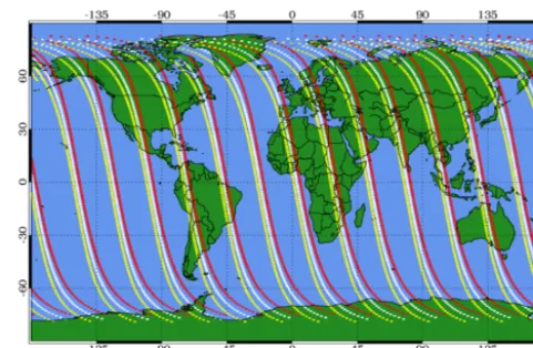
Figure 1.Daily coverage provided by the OMPS LP instrument mounted on the SNPP satellite. The tangent point for the LOS cor-responding to each observation is indicated, with red, white, and yellow circles depicting the left, center, and right slit observations, respectively.
the potential for increased geographic coverage as compared to SOT (but with a much dimmer source of light). Compar-isons of GOMOS stellar occultationβaretrievals to SAGE II, SAGE III, and POAM IIIβa data indicate agreement at the 10–25 % level in the lower stratosphere (Vanhellemont et al., 2010).
The lack of global stratosphericβa profile measurements from SOT since the SAGE II, POAM III, and Meteor-3M SAGE III missions ended (in 2005, 2005, and 2006, respec-tively) has left a vacancy. Limb-scattering (LS) data have been combined with occultation data (Rieger et al., 2015) to produce a merged time series, which will aid in tracking the evolution of aerosol plumes from volcanic eruptions that contribute aerosol to the upper troposphere and lower strato-sphere (UTLS) (Andersson et al., 2015). After an absence of over a decade, the recent installation of a SAGE III in-strument on the International Space Station (Cisewski et al., 2014) in February 2017 promises to resume the valuable SOT data set for stratosphericβamonitoring.
1.2 Limb-scattering (LS) measurements
Several recent missions have provided LS measurements, including the Optical Spectograph and InfraRed Imaging System (OSIRIS) (Llewellyn et al., 2004), the Scanning Imaging Absorption spectroMeter for Atmospheric Cartog-rapHY (SCIAMACHY) (Bovensmann et al., 1999), Meteor-3M SAGE III (Mauldin et al., 1998) (which made LS mea-surements in addition to occultation meamea-surements), and the Ozone Mapping and Profiler Suite (OMPS) Limb Profiler (LP) (Flynn et al., 2006). These instruments measure pro-files of the LS sunlight across the ultraviolet (UV), visible, and near-infrared (NIR) spectral regions.
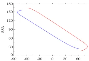
hemi-Figure 2.The single-scattering angle (SSA, or2) as a function of latitude for the SNPP OMPS LP instrument. June and December solstice conditions are illustrated by the red and blue lines, respec-tively. Note that near-polar latitudes may be observed twice (during the ascending and descending nodes of the orbit), which provides useful diagnostic information.
sphere, permitting much better spatial coverage and sam-pling than SOT measurements. But LS retrievals of strato-spheric βa are significantly more challenging, requiring ra-diative transfer (RT) models to simulate the diffuse radiation field, which must include all orders of atmospheric scatter-ing as well as surface reflection. Careful tangent height reg-istration of the measured radiance profiles (Moy et al., 2017) and cloud screening (Chen et al., 2016) are also required. The LS radiance is also susceptible to stray-light (SL) con-tamination (see Fig. 2 of Rault, 2005). Finally, the LS ra-diance depends upon both the scattering properties (espe-cially the phase function) and the extinction coefficient for the aerosols, while occultation measurements are only sensi-tive to the latter property.
Each LS mission team has developed its own methodol-ogy to retrieve stratospheric βa profiles from limb radiance measurements, but all of the retrieval algorithms involve the comparison of measured LS radiance profiles with simulated radiance profiles that are generated by a RT model. In the case of OSIRIS, the “color index” of measured LS radi-ances at 470 and 750 nm is compared to radiradi-ances calculated by the SASKTRAN (Bourassa et al., 2008a; Zawada et al., 2015) model. The evolution of βa during the OSIRIS mis-sion has been investigated in a series of papers (Bourassa et al., 2007; Bourassa et al., 2010; Bourassa et al., 2012). Com-parison between version 5 OSIRIS retrievals and the version 4 SAGE III record indicates agreement to within 10 % for βa in the 15–25 km altitude range (Bourassa et al., 2012). The retrieval of aerosol size information from OSIRIS data has also been investigated (Bourassa et al., 2008b; Rieger et al., 2014) to produce the version 6 OSIRIS aerosol prod-uct. The version 6 algorithm combines the infrared imager 1.53 µm channel with OSIRIS data to allow retrieval of both βa and aerosol mode radius, based on an assumed aerosol mode width value.
For the SCIAMACHY mission, the initial βa retrievals were performed by (Taha et al., 2011), using a modified
ver-sion of the algorithm under development for the eventual OMPS LP mission (Rault and Loughman, 2013). (Ovigneur et al., 2011) present an approach to retrieve stratospheric aerosol number density from SCIAMACHY LS data in the O2 A-band. More recent work (Ernst et al., 2012; Ernst, 2013; Von Savigny et al., 2015) describes an approach that uses the color-index approach introduced by (Bourassa et al., 2007). The global average difference between SAGE II (ver-sion 7) and SCIAMACHY (ver(ver-sion 1.1)βadata is 10 %, with larger relative differences (up to 40 %) at specific latitudes and altitudes (Von Savigny et al., 2015). The SCIATRAN RT model (Rozanov et al., 2014) provides the radiance simula-tions in this case.
The SAGE III instrument that flew on the Meteor-3M satellite made LS measurements as a research product, from which retrievals of ozone (Rault, 2005) and aerosol (Rault and Loughman, 2007) were derived. These retrieval al-gorithms were the predecessors for the initial OMPS LP algorithm (Rault and Loughman, 2013), which used the Gauss–Seidel limb-scattering (GSLS) RT model described in (Loughman et al., 2004) to provide the simulated radiances. Comparison to coincident SAGE II SOT data indicated bias <5 % and precision=25–50 % forβaretrievals from SAGE III LS data (Rault and Loughman, 2007).
Theβaretrieval algorithm described by (Rault and Lough-man, 2013) was applied to early OMPS LP observations. It was modified slightly to assess the aftermath of the Chelyabinsk bolide explosion, as documented by (Gorkavyi et al., 2013). This paper describes the new OMPS LP Ver-sion 1 (V1)βaretrieval algorithm. Section 2 briefly describes the OMPS instruments (particularly the LP instrument) and the Suomi National Polar-Orbiting Operational Environmen-tal Satellite System Preparatory Project (SNPP) satellite on which OMPS was initially installed. Section 3 focuses on the necessary radiance calculations, while Sect. 4 describes the retrieval algorithm in detail. Section 5 contains error analysis of the retrieved aerosol extinction profiles. Finally, a prelimi-nary evaluation of the retrieval results is presented in Sect. 6. We conclude with a summary and description of proposed future work in Sect. 7.
2 The OMPS LP Instrument
obser-Figure 3.The aerosol phase function (for the2values shown in Fig. 2) as a function of latitude for the SNPP OMPS LP instrument. June and December solstice conditions are illustrated by the red and blue lines, respectively. Due to the variation of the aerosol phase function with latitude and season, the SNPP OMPS LP observations are most sensitive to aerosols in the NH winter and least sensitive to those in the SH. The aerosol size distribution described in Table 1 for the V1 aerosol extinction retrieval algorithm is assumed.
vations (called the “center slit”) is oriented along the orbital track, while the other two sets (called the “left” and “right” slits) are offset by 4.25◦from the orbital track. The ground track of the resulting sequence of observations is illustrated in Fig. 1.
OMPS LP is installed in a fixed orientation relative to the SNPP spacecraft, which is in a sun-synchronous orbit with a 13:30 ascending node and mean altitude of 833 km above the Earth’s surface. As a result of this orientation, the single-scattering angle (2) observed by the LP instrument varies with latitude as shown in Fig. 2. Most notably, Northern Hemisphere observations (with latitude>0◦) generally cor-respond to forward-scattered beams (2 <90◦), while South-ern Hemisphere observations (latitude <0◦) correspond to backscattered beams (2 >90◦). As a result, the relative strength of the aerosol scattering signal is much larger in Northern Hemisphere OMPS LP measurements, as shown in Fig. 3: the aerosol phase function (Pa) increases by a fac-tor of approximately 50 over the course of a typical orbit, as the SNPP satellite travels from its southernmost observation to its northernmost observation. (All observations for which the solar zenith angle at the tangent pointθT <85◦are
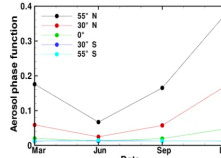
pro-cessed by the OMPS LP V1 software.) The variation of the Pa at several latitudes over the course of a year due to the OMPS LP orbit is shown in Fig. 4.
The OMPS LP instrument permits radiance observations for the 290–1000 nm wavelength range. Dispersion is pro-vided by a prism, which provides images whose spectral res-olution varies greatly with wavelength (from≈1 nm in the UV to ≈30 nm in the NIR). At the wavelength of interest for the V1βaretrieval algorithm (675 nm), the spectral reso-lution is 15 nm. For further information about the OMPS LP instrument characteristics, please consult (Flynn et al., 2006), (Rault and Loughman, 2013), and (Jaross et al., 2014).
Figure 4.The seasonal variation of the aerosol phase function at several latitudes for the SNPP OMPS LP orbit. The aerosol size dis-tribution described in Table 1 for the V1 aerosol extinction retrieval algorithm is assumed.
3 Radiance calculation
3.1 The GSLS radiative transfer model
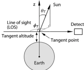
The GSLS RT model is built from the previous models de-scribed by (Herman et al., 1994, 1995), as summarized in (Loughman et al., 2004). The model atmosphere is spec-ified by input pressure, temperature, absorbing gas num-ber density, andβa profiles. Radiances are calculated using Rayleigh and Mie scattering cross sections at 675 nm, using the user-provided aerosol microphysical and optical prop-erties. Ozone cross sections are averaged over the spectral width of the OMPS LP bandpass (15 nm). This approach is significantly faster than performing a full radiance convolu-tion, and it produces radiance errors<1 %. The viewing ge-ometry is specified by the solar zenith angle and relative az-imuth angle at the tangent point (TP) for the LOS, denoted byθT andφT, respectively, and illustrated in Fig. 5.
The GSLS model calculates radiances at several wave-lengthsλ and tangent heightsh. For single-scattering (SS) calculations, the solar beam attenuation is calculated to each point along the LOS, including the curvature of the spherical atmosphere as well as the variation of solar zenith angle and solar beam attenuation along the LOS. The attenuation of the scattered beam along the LOS is also calculated accounting for the curvature of the atmosphere. Recent updates to the GSLS model described in (Loughman et al., 2015) reduce SS radiance errors that were as great as 4 % in the (Loughman et al., 2004) comparisons to the 0.3 % level.
dif-Figure 5.Illustration of the limb-scattering viewing geometry, in-cluding definitions of the tangent altitudehand tangent point. The solar zenith angle and solar azimuth angle at the tangent point are indicated byθT andφT, respectively. Adapted from Fig. 1 of
(Grif-fioen and Oikarinen, 2000). Note that a frequently committed error in the definition ofφT (Griffioen and Oikarinen, 2000; Loughman
et al., 2004; Bourassa et al., 2008b) has been corrected: a beam with
2=0◦(scattered exactly forward) hasφT =0◦.
fuse upwelling radiance (DUR) from below the LOS pro-vides the primary source of illumination that produces MS photons, containing the combined effects of molecular scat-tering, aerosol scatscat-tering, cloud scatscat-tering, and surface re-flection. For the V1 βa retrieval, the DUR is estimated as described in Sect. 3.2.
The MS source function is calculated at one or more points along the LOS using the pseudo-spherical version of the RT model described by (Herman et al., 1994, 1995). In the (Loughman et al., 2004) GSLS model, the MS source func-tions were calculated only at the TP (solar zenith angle=θT).
This was updated in (Loughman et al., 2015) to calculate the MS source functions at multiple solar zenith angles along the LOS, increasing the accuracy of the MS radiances. Total ra-diance errors that had reached 10% in the (Loughman et al., 2004) comparisons decrease to 1–3 % in the updated com-parisons presented by (Loughman et al., 2015).
The GSLS model described by (Loughman et al., 2004) was used for retrieval applications on missions including SOLSE/LORE (Flittner et al., 2000), SAGE III (Rault, 2005; Rault and Taha, 2007; Rault and Loughman, 2007), GOMOS (Taha et al., 2008), SCIAMACHY (Taha et al., 2011), and OMPS LP (Rault and Loughman, 2013). These retrieval al-gorithms generally performed well despite the shortcomings of the (Loughman et al., 2004) version of the GSLS model, but development of a more accurate version of the GSLS model was considered desirable to improve the algorithms further, as well as for the purpose of interpreting residu-als (differences between measured radiances and radiances calculated for the desired model atmosphere). The (Lough-man et al., 2015) version of GSLS has therefore been imple-mented for the V1 algorithm described in this paper.
3.2 The diffuse upwelling radiance (DUR)
The horizontal extent of the limb LOS covers thousands of kilometers, and the underlying scene generally includes vari-able surface types, broken clouds at various locations and levels, etc. The current GSLS model lacks the capability to model the full complexity of such a scene, even if its prop-erties were known. To estimate the DUR, the V1βaretrieval algorithm uses a simple Lambertian model of the reflecting surface, characterized by its reflectivityR. Radiances sim-ulated by the GSLS RT model using a Lambertian surface (placed at sea level) are used to estimate an effective scene re-flectivity from a measurement, by tuning the value ofRused in the GSLS model until the calculated radiance matches the measured value for a given set of viewing and illumination conditions.
TheRvalue at which the calculations match the measure-ment is sometimes called the “Lambert-equivalent reflectiv-ity”, or LER. It does not equal the true reflectivity of the sur-face, since the scene generally contains clouds, aerosols, etc. below the LOS that are not properly captured in the GSLS model atmosphere, and variations in terrain height are also ignored. This approach has been extensively used for nadir-viewing applications such as ozone profile retrievals from the SBUV satellite series and ozone total column retrievals from the TOMS satellite series (Heath et al., 1975), and it was sug-gested by (Mateer et al., 1971). Approximate treatment of DUR in the V1 OMPS LPβa retrieval algorithm is justified by the relative insensitivity of the normalized radiances used by theβaretrieval to DUR, as demonstrated in Sect. 3.4.
Finally, note that the model atmosphere for the GSLS model used in the V1βa retrieval algorithm is constrained to be one-dimensional (i.e., the atmospheric properties vary only with altitude). A two-dimensional SS version of GSLS (allowing atmospheric properties to vary along the LOS as well as with altitude) has recently been developed (Lough-man et al., 2016), and a full MS version of this model is cur-rently under development.
3.3 Aerosol properties
The LS radiance is affected by several aerosol properties. The V1 algorithm described in this paper employs assumptions for several of these properties in order to deduce theβabased on observations of the LS radianceI(λ,h).
3.3.1 Aerosol shape and optical properties
Table 1. Aerosol optical properties and aerosol size distribution (ASD) assumed in the V1 OMPS LP aerosol extinction retrieval.
Real aerosol refractive index 1.448
Imaginary aerosol refractive index 0 Aerosol median radius (fine mode),r1 0.09 µm
Aerosol mode width (fine mode),σ1 1.4
Aerosol median radius (coarse mode),r2 0.32 µm
Aerosol mode width (coarse mode),σ2 1.6
Aerosol coarse-mode fraction,fc 0.003
Aerosol scattering cross section (at 675 nm) 1.50×10⁻¹⁰cm2
various tropospheric aerosols that enter the stratosphere). However, the assumption that “aged” aerosol in the Junge layer is dominated by such H2SO4droplets agrees with ob-servations dating back to the earliest studies of stratospheric aerosol (Junge et al., 1961b) and is assumed in all previ-ous LSβaretrieval algorithms. The assumption is less sup-portable under “perturbed” stratospheric conditions (such as the immediate aftermaths of volcanic eruptions), as noted by (Vernier et al., 2016), or at the upper and lower boundaries of the Junge layer, which may have more meteoric content above and more tropospheric aerosol near the tropopause. 3.3.2 Aerosol size distribution (ASD)
In the V1 algorithm, the ASD is modeled as a bimodal log-normal (LN) distribution, as specified in Table 1. This ASD is defined by Eq. (1):
dN (r) dr =
2 X
i=1 Ni r
√
2πlnσi
exp (
−1
2 ln
(r/ri)
lnσi 2)
. (1)
Five independent parameters are required to specify the shape of the bimodal LN ASD: two median radii (r1 and r2), two mode widths (σ1 and σ2), and one more parame-ter indicating the relative sizes of the aerosol concentration associated with each mode (N1,N2). In this work, the mode with the smaller median radius value (r1) is called the “fine mode”, while the other mode is the “coarse mode”. There-fore the relative sizes of the aerosol modes are described by the “coarse-mode fraction”fc=N2/(N1+N2). (Changes in the absolute values ofN1andN2alter the magnitude of the βafor a given distribution but do not change the shape of the ASD for a givenfcvalue.)
The ASDs used in several other LSβaretrieval algorithms are given in Table 2. These properties have typically been taken from the long record of balloon-borne optical particle counter (OPC) data provided by T. Deshler’s group at the University of Wyoming. But this data set indicates that the ASD varies considerably with time, location, and altitude. For example, the V1.1 SCIAMACHY ASD (Von Savigny et al., 2015) is taken from Fig. 3c in (Deshler et al., 2008) (ex-cluding the coarse mode). (Bourassa et al., 2007) and (Rieger et al., 2014) cite (Deshler et al., 2003) as the source of the
Figure 6.Illustration of the aerosol size distributions used in several recent LS aerosol extinction retrieval algorithms, including OSIRIS (V5), SCIAMACHY (V1.1), and OMPS (V0.5 and V1). The aerosol size distribution studied by Nyaku (2016) is also represented.
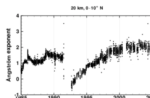
Figure 7. Ångström exponentα(525/1020) derived from SAGE II SOT measurements during its measurement history. This pic-ture corresponds to measurements at altitude 20 km for the 0– 10◦N latitude bin. Cases for which the measured aerosol extinc-tion at 1020 nm<4×10⁻⁶km were excluded from this analysis (L. Thomason, private communication).
V5 OSIRIS ASD, which resembles Fig. 5b of that reference (again excluding coarse-mode particles). (Nyaku, 2016) uses the 2012–2013 data provided by the University of Wyoming website for Laramie as the basis of the bimodal LN ASD for sensitivity studies, as cited earlier in (Loughman et al., 2015). Unfortunately, the OPC data corrections described by (Kovilakam and Deshler, 2015) occurred after the OSIRIS, SCIAMACHY, and Nyaku ASDs described in this paragraph were defined, so none of those ASDs reflect the corrected version of the OPC data.
Table 2.Aerosol size distributions assumed in several recent LS aerosol extinction retrieval algorithms.
Mission Source r0(µm) σ α(525/1020)
OMPS (V0.5) Loughman et al. (2015) 0.06 1.73 2.34 OSIRIS (V5) Bourassa et al. (2007) 0.08 1.6 2.44 SCIAMACHY (V1.1) Von Savigny et al. (2015) 0.11 1.37 2.82 Nyaku Nyaku (2016), fine mode 0.05105 1.43833 2.07
(Nyaku, 2016), coarse mode 0.2025 1.15
Figure 8. Variation of Ångström exponent α(525/1020) with aerosol properties for the V1 OMPS LP aerosol extinction re-trieval algorithm characteristics. Each curve shows the variation of
(α(525/1020)withfc for a given set of median radii and mode
widths. In addition to the “base” curve (which uses the V1 char-acteristics listed in Table 1), several curves show how the value of
α(525/1020)changes as the values ofr1, σ1, r2, andσ2(in Table 1)
are perturbed by±10 %.
Sect. 5.2. A single-mode LN ASD is assumed in stratospheric βaretrievals by the V5 OSIRIS (Bourassa et al., 2007), V1.1 SCIAMACHY (Von Savigny et al., 2015), and intermediate V0.5 OMPS LP retrievals, as shown in Table 2. The assumed median radius (r0), mode width (σ), and resulting Ångström coefficientα(525/1020)(defined below in Eq. 2) are shown in Table 2, and several single-mode and bimodal LN ASDs are shown in Fig. 6. Table 2 also includes the properties of the bimodal LN ASD analyzed by (Nyaku, 2016).
α(525/1020)=−ln
βa(525 nm)/βa(1020 nm) ln
525/1020 (2)
For the V1 OMPS LP βa retrieval algorithm, we introduce the added complexity of the bimodal LN ASD because it generally describes the properties of stratospheric aerosol observations better (Thomason and Peter, 2006). The fine-and coarse-mode properties of the V1 OMPS ASD (given in Table 1) were selected based on the data found in Ta-ble 1a of (Pueschel et al., 1994). These observations were taken on 23 August 1991, in the aftermath of the eruption
of Mt. Pinatubo, and are based on in situ measurements by impactor samplers flown on an ER-2 aircraft in the lower stratosphere. The intention of this choice was to keep the ob-served fine mode for stratospheric aerosols (with properties broadly similar to the single-mode LN ASDs shown in Ta-ble 2), while introducing the possibility of a coarse mode of larger aerosols. The recent eruption of Mt. Pinatubo causes fc=0.36 in the selected (Pueschel et al., 1994) data, which is much larger than one would expect in the background stratosphere. Therefore the relative prominence of the coarse mode was reduced for the V1 OMPS LPβa algorithm by tuning thefc value, based on the following considerations drawn from the available stratospheric aerosol data record:
1. The SAGE satellite series (particularly SAGE II) pro-vides a long-term record ofβaprofiles for stratospheric aerosols at several wavelengths. The βa wavelength variation can be expressed by the Ångström coefficient α, which is defined by Eq. (2) based on observations ofβaat 525 and 1020 nm. The SAGE II zonal meanα value for the tropics at 20 km is shown in Fig. 7. Except for volcanically perturbed periods, the observedαvalue at this altitude is relatively constant atα≈2. This value tends to grow with altitude above the peak of the strato-spheric aerosol layer, approachingα≈2.5 at 30 km. 2. Figure 8 shows how α varies with coarse-mode
frac-tionfc, for fine- and coarse-mode fraction values in the vicinity of the V1 OMPS LP ASD values (r1,σ1,r2, and σ2in Table 1). For these assumed fine- and coarse-mode properties, the value ofαis extremely sensitive tofc. If one assumes that the fine and coarse modes are correctly specified, this implies that fc can be determined with great precision based on the observed value ofα. The V1 OMPS LPβaretrieval algorithm usesfc=0.003 in conjunction with the (Pueschel et al., 1994) values of r1, σ1, r2, andσ2to produceα=2.
Figure 9. The aerosol phase function at 675 nm as a function of SSA (or2) for the aerosol size distributions listed in Tables 1–2.
Figure 10.The aerosol phase function at 756 nm as a function of SSA (or2) for the aerosol size distributions listed in Tables 1–2.
whenr1,σ1,r2, andσ2remain at their default values (shown in Table 1), butfcis varied: in one casefc=0.0012 (produc-ingα=2.5), while in the other casefc=0.006 (producing α=1.5). As expected, thePabecomes more “Rayleigh-like” asαincreases, but the change inPais relatively modest (gen-erally<10 %) except for small scattering angles (2 <30◦). The impact of thePais discussed further in Sect. 5.2. 3.4 Properties of altitude-normalized radiances
(ANRs)
As explained in Sect. 4.1, the V1 algorithm uses ANRs rather than radiances to define the measurement vectory. The ANR is defined as ρ=I (λ, h)/I (λ, hn), with the radiance at the tangent heighthof interest divided by the radiance at a
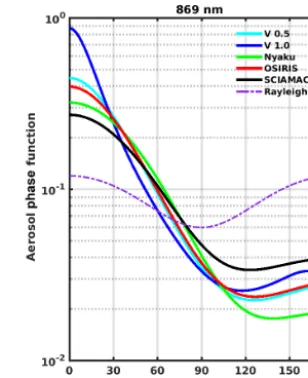
se-Figure 11.The aerosol phase function at 869 nm as a function of SSA (or2) for the aerosol size distributions listed in Tables 1–2.
Figure 12.The aerosol phase function at 1020 nm as a function of SSA (or2) for the aerosol size distributions listed in Tables 1–2.
lected normalization tangent heighthn> h. For the V1 algo-rithm,hn=40.5 km. In Fig. 14,ρat 675 nm is calculated for a range of scattering angles using the V1 OMPS LP ASD. Theβa, ozone, pressure, and temperature profiles are fixed for the radiance calculations shown in Fig. 14, in order to isolate the dependency ofρon2andR. In Fig. 14,handhn are 25.5 and 40.5 km, respectively.
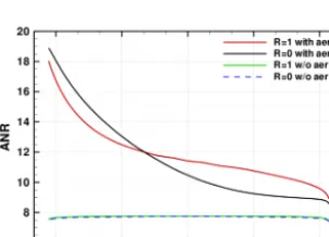
When aerosols are excluded from the model atmosphere, Fig. 14 shows that theρis insensitive to both2andR. But when aerosols are included, several effects emerge:
Figure 13.Aerosol phase function sensitivity to perturbations of the aerosol size distribution, using the V1 aerosol size distribu-tion as a baseline. Note that the±10 % perturbations ofr1, σ1, r2,
and σ2also involved adjustments offcto keepα≈2. Two other
perturbations are shown, in which the values ofr1, σ1, r2, andσ2
remain at the V1 aerosol size distribution values, but fc is
var-ied: CMF0.0012AE2.5 (red line) indicates thatfc=0.0012
(pro-ducingα=2.5), and CMF0.0060AE1.5 (black line) indicates that
fc=0.06 (producingα=1.5)
Figure 14.Altitude-normalized radiances (ANR, orρ) at 675 nm as a function of SSA (or2) under aerosol-free and aerosol conditions, with both non-reflecting (R=0) and perfectly reflecting (R=1) surface conditions. The values ofhandhnare 25.5 and 40.5 km,
respectively.
Pa is divided by the Rayleigh phase functionPR. The phase function ratio varies with2as shown in Fig. 15. 2. ρalso shows some dependence onRwhen aerosols are
included. However, this effect is relatively small com-pared to the effect ofRon the radiance, which can reach 100 % at large values ofR.
3. As noted above,ρdecreases with increasing2, show-ing similar behavior to the Pa/PR ratio when the un-derlying scene is dark. But this decrease becomes more gradual for brighter scenes, in which theρdependence on2is flattened out. As the underlying scene becomes brighter, the limb radiance is influenced more by DUR.
Figure 15.The ratio of APF (orPa) to RPF (orPR) as a function
of SSA (or2) for the V1 OMPS LP aerosol size distribution. This ratio declines by a factor of≈50 between forward (2=0◦) and backward (2=180◦) scattering conditions.
Figure 16.Daily zonal mean aerosol scattering index (ASI, ory) measured by the SNPP OMPS LP instrument. This picture corre-sponds to center slit observations on 23 September 2015. Thexaxis is labeled with both the event number (solid) and tangent point lat-itude (italics). The color scale is nonlinear, designed to highlight relatively smallyvalues in the SH.
This upwelling radiation illuminates the LOS from a va-riety of directions, reducing the influence of the solar scattering angle 2on ρ. As a result, ρ becomes less sensitive to the details ofPa(2)asRincreases.
4 Retrieval algorithm
4.1 Aerosol scattering index (ASI)
The V1 algorithm uses the ASI as its measurement vector y. The ASI is defined asy(λ, h)=(ρm−ρR)/ρR, whereρm
is the measured ANR andρRis the ANR calculated
a climatological ozone profile to account for the weak ozone absorption at 675 nm. The ozone estimate is then updated at the final step of the retrieval, as described in Sect. 4.3.
For an optically thin LOS, the ANR is approximately the sum of ρa (the ANR due to aerosol scattering) + ρR (the
ANR due to Rayleigh scattering). In that case, the measured ANR=ρm≈ρa+ρR, and therefore the ASI=y≈ρa/ρR. It is also true under these conditions that ρa≈βa×Pa. However, under more general conditions the scattering con-tributions cannot be treated independently: attenuation of Rayleigh-scattered photons by aerosols (and vice versa) can causeyto become negative at some altitudes. This indicates that the aerosol attenuation effect has exceeded the aerosol scattering effect. This behavior can be seen in Fig. 16, partic-ularly at the southern end of the orbit (where the OMPS LP aerosol signal is weakest). Figure 16 shows a strong hemi-spheric contrast iny, which simply reflects the variation of Pawith2.
Finally, note that use ofy(and its dependence onρ) is best suited for a circumstance in which an “aerosol-free” layer lies above the aerosols of interest. That implicit assumption is consistent with the fact that H2SO4droplets evaporate com-pletely in the 30–35 km altitude range, due to the warmer stratospheric temperatures at that level (Toon and Pollack, 1973). But use ofy makes us unable to detect aerosol scat-tering that has a constant mixing ratio with height (relative to molecular scattering), so the contributions of other aerosol sources such as meteoric smoke (Hervig et al., 2009) require further investigation.
4.2 Inverse model
The V1 algorithm uses OMPS LP radiance measurements at a single wavelength (675 nm) to estimate the βa profile. This wavelength was selected primarily to provide aerosol information to the V2.5 ozone code that uses a wavelength triplet (consisting of 510, 600, and 675 nm) to retrieve the ozone profile (Kramarova et al., 2017). Since both βa and Pa have strong wavelength dependence in the stratosphere, aerosol profiles derived from a wavelength near the Chappuis ozone band are expected to minimize aerosol-related errors in the ozone retrieval.
Several additional advantages make selecting a wave-length near 700 nm optimal for OMPS LP aerosol retrievals. Wavelengths<500 nm feature weak ozone absorption, but large Rayleigh scattering obscures the aerosol signal. OMPS LP also measures wavelengths longer than 675 nm, but these tend to be more affected by internal instrument SL. The OMPS LP instrument was designed and characterized pri-marily with the goal of ozone retrieval, and therefore suc-cessful characterization of SL at the longer wavelengths is an ongoing project. Longer wavelengths are also more sensitive to the highly uncertain ASD than 675 nm (see Figs. 10–12), making 675 nm attractive forβaretrievals.
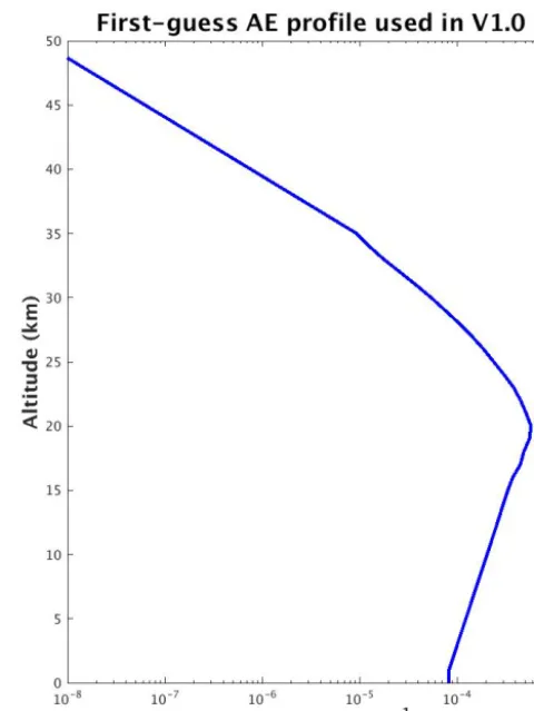
Figure 17.The first-guess aerosol extinction (or AE) profile used in the V1 OMPS LP aerosol extinction retrieval algorithm.
The V1 algorithm uses the Chahine nonlinear relaxation method (Chahine, 1970) to obtain theβafrom the OMPS LP measurements. Since ASI is roughly proportional toβa, we use ASI as the measurement vectory, which is updated itera-tively as shown in Eq. (3), based on the notation of (Rodgers, 2000), Sect. 6.8:
xni+1=xni y
m i
yni . (3) The symbol xn
i represents the state vector (βa) at altitude zi afterniterations of the retrieval algorithm. The
measure-ment vectorym
i represents the measuredyat tangent height hi=zi. The GSLS RT model calculates the ASI vectoryni
at each iteration, using theβa profile given byxni. The iter-ative process is initialized with a nominal first-guess aerosol profile x0i derived from 2000–2004 SAGE data (shown as Fig. 17), which does not vary with latitude or season. Fig-ure 18 shows the daily zonal meanβa retrieved from they values shown in Fig. 16. Note that the hemispheric asymme-try shown in theyfigure is not repeated in theβafigure.
The retrieval is constrained to limit changes within a sin-gle iteration: xi can increase by no more than a factor of
Figure 18.Daily zonal mean aerosol extinction for center slit ob-servations on 23 September 2015 (derived from theymeasurements shown in Fig. 16).
Figure 19.Daily zonal mean aerosol scattering index (ASI, ory) residuals for center slit observations on 23 September 2015 (derived from theymeasurements shown in Fig. 16).
each iteration. The algorithm executes just three iterations, which constrains the final solution at each altitudexi3within the range of values xi0/125≤xi3≤8xi0. The retrieval algo-rithm setsxi to zero for observations with weak aerosol
sig-nals (whereymi <0.01). Data at altitudes for which a cloud has been detected by the algorithm described by (Chen et al., 2016) are flagged. An example of the residual (difference between measured and calculated)y is presented in Fig. 19, which demonstrates general convergence to the±2 % level except at altitudes <15 km and for regions near the South Pole (where the SNPP OMPS LP aerosol signal is weakest). 4.3 Ozone correction
The V1βaalgorithm operates independently from the ozone retrieval algorithm (Kramarova et al., 2017). As noted in Sect. 4.1, a climatological ozone profile is assumed during the iterations of theβaretrieval. After those three iterations are complete, an approximate ozone correction is applied as follows. Forλ1, λ2, andλ3=510, 600, and 675 nm, respec-tively, we defineY (h, λi)=Yi in terms of the measured
ra-diance (Im) and the calculated radiance (Ic) at each wave-length:
Yi=ln I
m(h, λi) Ic(h, λi)
. (4)
Based on these threeY values, we define a three-parameter fit:
Yi=a+bλi+cσi, (5)
whereσi = the ozone absorption cross section averaged over
the OMPS LP bandpass centered atλi. Thecparameter
rep-resents the sensitivity of the ozone slant column density with respect to the first guess and can be determined from Eq. (6): c=(Y2−Y1)(λ3−λ2)−(Y3−Y2)(λ2−λ1)
(σ2−σ1)(λ3−λ2)−(σ3−σ2)(λ2−λ1)
. (6)
The ozone-corrected value of Y at 675 nm is therefore de-noted byYc(λ3):
Yc(λ3)=Y (λ3)exp [cσ (λ3)]. (7) A similar correction is also applied to the value ofY at the normalization tangent height to obtainYc(hn, λ3).
5 Error analysis
This section describes the most significant categories of un-certainty that we anticipate will limit the accuracy and preci-sion of the V1 retrievals. Quantitative estimates of the antic-ipated error are provided when possible, but a full algorithm error budget is beyond the scope of this study. Unfortunately, many uncertainties are difficult to quantify for the full range of possible conditions.
To provide an overall context for assessing the signifi-cance of various error sources, we begin by detailing the cess used to estimate the atmospheric number density pro-file used in the V1βaretrieval algorithm. This profile is de-rived from the operational geopotential height product pro-vided by the NASA Global Modeling and Assimilation Of-fice (GMAO), which has reduced quality at altitudes above 35 km. The resulting uncertainty has been estimated by com-parisons with the Modern-Era Retrospective analysis for Re-search and Analysis, Version 2 (MERRA-2) fields, which in-corporate Microwave Limb Sounder (MLS) temperature pro-files above 35 km (Gelaro et al., 2017). This comparison in-dicates both noise and bias at the 1–2 % level for calculation of radiances ath=40 km.
We therefore neglect error sources that exist below this 1– 2 % “floor” level and concentrate on error sources that exceed that threshold. This criterion eliminates both stray light and random error associated with the OMPS LP measurements, which typically are<1 %.
5.1 Uncertainty due to measurement errors
Figure 20.Contour plot showing the ratio of the Ångström coeffi-cientαfor a given aerosol size distribution to the V1 aerosol size distributionα≈2. Cases for which this ratio is within±5 % of 1 are highlighted in white. The coarse-mode properties are fixed in this example at the V1 aerosol size distribution values (r2=0.32 µm; σ2=1.6), while the fine-mode properties vary in the vicinity of the
V1 aerosol size distribution values (r1=0.09 µm;σ1=1.4). Red
circles indicate the individual cases calculated to create this figure.
the SL error athn. OMPS LP stray light acts roughly as an additive effect (Jaross et al., 2014) and therefore affects the measured radiance athnmuch more strongly than the other radiances that form y, due to the roughly exponential de-crease of I with tangent height. Internal analysis suggests that this error is 1 %, and it therefore produces fractional er-ror inx=0.01/y. Stray-light error therefore becomes most significant at altitudes and latitudes whereyis small(<0.1). As shown in Fig. 16, this condition is most likely to occur near the top of the Junge layer (h≈35−−40 km) and/or near the South Pole (where SNPP OMPS LP provides unfavorable viewing conditions forβaretrieval, with large2producing smallPavalues).
5.2 Uncertainty due to radiative transfer limitations The GSLS radiative transfer model used in the V1 OMPS LP βaretrieval algorithm contains several limitations that affect the retrievedβaprofiles. The most significant issues are listed below, in order of priority.
1. Uncertainty in the aerosol scattering phase functionPa As described in Sect. 3.3.2, we have selected a bimodal LN ASD to calculate the assumedPaused in the V1βa retrieval algorithm. However, we cannot expect that any single ASD will be correct for the full range of OMPS LP observations. And even if a single ASD were suit-able, many plausible combinations ofr1, σ1, r2, σ2,and fcexist that would fit the criterion stated in Sect. 3.3.2 (α≈2) equally well, as shown in Fig. 20. Whether these “plausible” ASDs produce significantly differentPa
val-Figure 21.The background contour plot is the same as in Fig. 20. This time, red circles appear only for cases in which the Ångström coefficient ratio is within±5 % of 1andthe aerosol phase func-tion is within±10 % of the V1 aerosol size distribution value at
2=60◦. Nearly every aerosol size distribution that satisfies the Ångström coefficient ratio criterion also satisfies the aerosol phase function criterion for this case.
Figure 22.Identical to Fig. 21 except that the aerosol phase function comparison is done for2=120◦. For this viewing geometry, the aerosol phase function criterion is much more useful in determining the aerosol size distribution properties: Note the smaller number of red circles (relative to Fig. 21), centered around the true values of
r1(0.09 µm) andσ1(1.4).
Since ρa is approximately proportional to Pa for opti-cally thin LOS, differences between the assumed and truePavalues map directly intoβaerrors in the V1 al-gorithm. Figure 22 therefore predicts that the OMPS LP βaretrievals for2=120◦will be greatly affected by the assumed ASD in the retrieval, while Fig. 21 shows that the OMPS LPβa retrievals for2=60◦will be nearly insensitive to the assumed ASD. The preceding analy-sis roughly estimates the possible error that may result in the V1 OMPS LP βa retrievals, but it provides no clear method to estimate the error in a single retrieval at a particular place, time, and altitude. This topic will be explored more thoroughly in a future publication. 2. Uncertainty due to LOS variation in atmospheric
prop-erties
As noted in Sect. 3.1, the RT model in the V1 OMPS LPβaretrieval assumes that the atmospheric properties vary only with altitude. This assumption is used to re-trieve βafor each measured image, independent of the neighboring images. But the maps of retrievedβa val-ues regularly feature large horizontal variations, partic-ularly latitudinal variations (see Fig. 18). Many such features persist at particular latitude ranges for which stratospheric dynamics are known to cause steep hori-zontal gradients inβaat a given altitude.
The viewing geometry of OMPS LP (looking back-wards along the sun-synchronous orbital track) exac-erbates this problem, due to the zonal gradients in βa seen in Fig. 18, but LOS variations of atmospheric prop-erties affect all limb-viewing retrieval methods. Past limb missions have developed a two-dimensional re-trieval strategy that allows variation of the retrieved quantity both along the LOS and with altitude. The MLS (limb emission) mission (Livesey and Read, 2000) and OSIRIS (LS) mission (Zawada et al., 2015) have made notable progress in this area. The V1 OMPS LP al-gorithm remains a 1-D solution (with βa varying only with altitude). This assumption is likely to affect the re-trieval most strongly at the edge of the tropics (whereβa tends to have a large horizontal gradient), in the North-ern Hemisphere (whereyvaries rapidly with2), and at the edges of a fresh volcanic cloud.
3. Uncertainty due to approximate treatment of DUR The limb LOS is illuminated from above (overwhelm-ingly by direct solar radiation) and from below (by pho-tons scattered within the underlying atmosphere and/or reflected by the underlying surface). The latter source of radiation is modeled as described in Sect. 3.2: A Lam-bertian surface is assumed to lie beneath the model at-mosphere (which is not updated outside the range at which theβa is retrieved during the iteration process). This assumption allows one to determineR, the
effec-Figure 23.LER retrieved from radiances ath=40 km (blue line) and 50 km (green line). Center slit observations from orbit 20234 are used in this example. Again, as noted in Fig. 14, the OMPS LP aerosol extinction retrieval is insensitive to LER.
tive Lambertian surface reflectivity that is consistent with the measured radiance athn=40.5 km.
This assumption provides a first-order estimate of the DUR, but this estimate will generally be imperfect for the following reasons:
a. The simple assumptions described above generally fail to represent the true conditions below a given LOS in multiple ways: the atmosphere will generally include clouds and aerosols below the LOS that are not in-cluded in the model atmosphere. The true bi-directional reflectance distribution model (BRDF) of the scene will also generally be non-Lambertian. In such cases, the up-welling radiation in the model calculation will have a different angular distribution than the upwelling radia-tion in the true atmosphere.
b. For an inhomogeneous underlying scene, the effective LER may also vary with h, due to the varying solid angle that contributes toI (h). The difference between LER (h=40 km) and LER (h=50 km) is typically slight (see Fig. 23), implying that this is a minor effect, but more research is needed to assess whether any sys-tematic relationships exist.
5.3 Inverse model errors
This section includes several effects unrelated to the radiative transfer model that affect the V1 OMPS LPβaretrieval, again listed in order of priority.
1. Large aerosol extinction
LS radiance will be more influenced by the LOS seg-ment nearest the sensor (see item 3 below).
2. Cloud detection algorithm
The current cloud detection algorithm (Chen et al., 2016) detects clouds well, but it sometimes also flags fresh volcanic aerosols as clouds. Since retrieval of such aerosols is quite complicated for several reasons dis-cussed earlier (LOS inhomogeneity, uncertainty about the appropriatePadue to a mixture of aerosol types and shapes, etc.), we have not attempted to fix this error. 3. Poor convergence
The algorithm often does not converge well for scenes in which theyhas large horizontal gradient. We believe that this occurs because of 2-D effects discussed earlier in Sect. 5.2, which produce an asymmetry in the LS ra-diance contribution function. Under optically thick con-ditions, the LS radiance will be influenced by the atmo-sphere near the satellite much more than the atmoatmo-sphere far from the satellite at a given altitude. This effect is illustrated in Fig. 6c of (Loughman et al., 2015). Fix-ing this problem will require the development of a 2-D aerosol algorithm.
5.4 Ozone correction errors
The 675 nm radiances used in the V1 OMPS LPβaretrieval algorithm lie within the Chappuis ozone absorption band, and therefore the βa estimate is influenced by possible dif-ferences between the true ozone profile and the ozone pro-file that is assumed in the calculation of yni in Eq. (3). We therefore apply the ozone correction described in Sect. 4.3 to reduce this source of error. This correction produces the largest percentage change in the retrievedβavalue when the following conditions are met:
1. the a priori ozone concentration differs significantly from the true ozone concentration,
2. yis relatively small for a givenβavalue, 3. theβavalue itself is small.
The first condition is most likely to occur for regions with highly variable ozone profiles. The second condition will prevail for regions that are viewed by OMPS LP at large2 values, where the correspondingPavalue is small. The third condition occurs primarily in regions with lowβavalues, typ-ically where sinking air prevails in the mid-stratospheric re-gion.
The largest ozone corrections therefore typically appear near the South Pole, where minima for both they andβaat a given altitude tend to occur, as shown in Figs. 16 and 18, respectively. The ozone profile also exhibits large variation in this region, partly due to the formation of the Antarctic spring ozone hole. Under these extreme conditions, the ozone
Figure 24. OMPS LP V1 (blue line) and OSIRIS V5.07 (red line) retrieved aerosol extinction daily zonal means at selected al-titudes from 2012 to 2016, at laal-titudes between 10 and 0◦S. The OSIRIS data set reports aerosol extinction at 750 nm, so the OMPS aerosol extinction was converted from 674 to 750 nm by using the Ångström coefficient consistent with the aerosol size distribution assumed in the OMPS LP V1 algorithm.
correction produces changes in the retrievedβavalue as large as 20 %. For a more typical case in the tropics, theβachanges by<3 % when the ozone correction is applied.
6 Preliminary evaluation of retrieval results
In this section, we will only present an early qualitative eval-uation of OMPS LP V1βadata in comparison with profiles derived from OSIRIS LS radiances and Cloud-Aerosol Li-dar and Infrared Pathfinder Satellite Observation (CALIPSO; Winker et al., 2009) backscattered lidar measurements. A de-tailed validation paper for the OMPS LPβaretrievals is in preparation.
instru-Figure 25. Monthly zonal mean aerosol extinction profiles at 750 nm derived from CALIPSO, OSIRIS, and OMPS LP measure-ments during the aftermath of the Kelut eruption in 2014.
ments clearly show the quasi-biennial oscillation (QBO) sig-nature of enhancedβavalues during easterly shear conditions of the QBO (Trepte and Hitchman, 1992) during early 2012, 2013–2014, and 2016, caused by enhanced aerosol lofting. The lower values ofβain 2012 and 2015 are associated with westerly shear conditions of the QBO, causing downward aerosol transport.
Figure 25 shows monthly zonal meanβaprofiles at 750 nm derived from CALIPSO, OSIRIS, and OMPS LP measure-ments during 2014. This time series is averaged from 5 to 0◦S, and altitudes 15–35 km are illustrated. CALIPSO data were provided by (Vernier et al., 2011) and (Vernier et al., 2015). The three instruments track Kelut injection of volcanic aerosol at 20 km and the upward lofting of the aerosol to higher altitudes (≈25 km) within a few months. The CALIPSO data are based on a series of narrow lidar swaths, so its coverage differs from OSIRIS and OMPS LP coverage. Vertical resolution differences might also explain some the differences seen among the three instruments.
7 Conclusions
The OMPS LP V1 aerosol extinction (βa) retrieval algorithm is summarized in this document. The V1 algorithm differs from the most recently published OMPS LP algorithm (given in Rault and Loughman, 2013) in several ways:
1. the βa profile is retrieved at a single wavelength, 675 nm;
2. the retrieval uses the (Chahine, 1970) solution method; 3. the assumed ASD is bimodal lognormal, guided by
the aerosol properties measured by (Pueschel et al., 1994) with the coarse-mode fraction tuned to produce Ångström coefficientα(525/1020)≈2.
The main motivation for these changes was to produce a simpler algorithm that works with the best-characterized OMPS LP radiances. The resultingβaprofiles are more sta-ble and permit more straightforward analysis of the radiance residuals. Initial comparisons with coincident OSIRIS and
CALIPSOβa data show similar spatial and temporal varia-tion over the lifetime of the OMPS LP instruments.
The accuracy of the absolute value of the OMPS LPβa re-mains variable, primarily due to uncertainty about the appro-priate ASD to be used. The V1 ASD selection was guided by the Ångström coefficient measured by SAGE II during vol-canically quiescent periods. But the lack of contemporaneous global observations of the ASD presents a significant chal-lenge for all LSβaretrievals, particularly for observations at 2 >90◦ (Southern Hemisphere conditions for OMPS LP). The recently launched ISS SAGE III instrument is capable of both SOT and LS observations, which should provide valu-able information to reduce uncertainty in thePa for strato-spheric aerosols.
Future work to improve the OMPS LPβa algorithm will begin by adding consideration of additional wavelengths. Longer wavelengths are sensitive to lower tangent heights that typically saturate at 675 nm due to interference by Rayleigh scattering and are also more sensitive to small aerosol signals (such as OMPS LP encounters in the South-ern Hemisphere). Additional wavelengths also will allow us to asses the self-consistency of the measuredβawavelength variation with the Mie theory prediction for the assumed ASD. A 2-D algorithm will also improve performance in the vicinity of large horizontal variations. The ability to allow the ASD to vary with height will also be valuable, given better ASD information.
Data availability. The retrieved profiles produced by the V1 OMPS LP aerosol extinction retrieval algorithm are publicly avail-able at the following site: https://ozoneaq.gsfc.nasa.gov/data/ozone/ (NASA, 2018).
The Suomi NPP daily files for the aerosol extinction product are labeled as “OMPS Limb Profiler –Suomi NPP – LP-L2–AER675-DAILY”.
Competing interests. The authors declare that they have no conflict of interest.
discussions, including Larry Flynn, Matt DeLand, Jack Larsen, and Tong Zhu. Finally, several summer research students contributed to studies that have improved this work, including Nelson Ojeda, Ryan McCabe, and Ashley Orehek.
Edited by: Christian von Savigny Reviewed by: two anonymous referees
References
Andersson, S. M., Martinsson, B. G., Vernier, J. P., Friberg, J., Brenninkmeijer, C. A., Hermann, M., van Velthoven, P. F., and Zahn, A.: Significant radiative impact of volcanic aerosol in the lowermost stratosphere, Nat. Commun., 6, 7692, https://doi.org/10.1038/ncomms8692, 2015.
Bertaux, J. L., Kyrölä, E., Fussen, D., Hauchecorne, A., Dalaudier, F., Sofieva, V., Tamminen, J., Vanhellemont, F., Fanton d’Andon, O., Barrot, G., Mangin, A., Blanot, L., Lebrun, J. C., Pérot, K., Fehr, T., Saavedra, L., Leppelmeier, G. W., and Fraisse, R.: Global ozone monitoring by occultation of stars: an overview of GOMOS measurements on ENVISAT, Atmos. Chem. Phys., 10, 12091–12148, https://doi.org/10.5194/acp-10-12091-2010, 2010.
Boucher, O.: On aerosol direct shortwave forcing and the henyey-greenstein phase function, J. Atmos. Sci., 55, 128–134, 1998. Bourassa, A. E., Degenstein, D. A., Gattinger, R. L., and
Llewellyn, E. J.: Stratospheric aerosol retrieval with opti-cal spectrograph and infrared imaging system limb scat-ter measurements, J. Geophys. Res.-Atmos., 112, D10217, https://doi.org/10.1029/2006JD008079, 2007.
Bourassa, A. E., Degenstein, D. A., and Llewellyn, E. J.: Re-trieval of stratospheric aerosol size information from OSIRIS limb scattered sunlight spectra, Atmos. Chem. Phys., 8, 6375– 6380, https://doi.org/10.5194/acp-8-6375-2008, 2008a. Bourassa, A. E., Degenstein, D. A., and Llewellyn, E. J.:
SASK-TRAN: A spherical geometry radiative transfer code for efficient estimation of limb scattered sunlight, J. Quant. Spec. Rad. Trans., 109, 52–73, 2008b.
Bourassa, A. E., Degenstein, D. A., Elash, B. J., and Llewellyn, E. J.: Evolution of the stratospheric aerosol enhancement following the eruptions of Okmok and Kasatochi: Odin-OSIRIS measurements, J. Geophys. Res., 115, D00L03, https://doi.org/10.1029/2009JD013274, 2010.
Bourassa, A. E., Rieger, L. A., Lloyd, N. D., and Degenstein, D. A.: Odin-OSIRIS stratospheric aerosol data product and SAGE III intercomparison, Atmos. Chem. Phys., 12, 605–614, https://doi.org/10.5194/acp-12-605-2012, 2012.
Bovensmann, H., Burrows, J. P., Buchwitz, M., Frerick, J., Noël, S., Rozanov, V. V., Chance, K. V., and Goede, A. P. H.: SCIA-MACHY: Mission Objectives and Measurement Modes, J. At-mos. Sci., 56, 127–150, 1999.
Brock, C. A., Hamill, P., Wilson, J. C., Jonsson, H. H., and Chan, K. R.: Particle Formation in the Upper Tropical Troposphere: A Source of Nuclei for the Stratospheric Aerosol, Science, 270, 1650–1653, https://doi.org/10.1126/science.270.5242.1650, 1995.
Chahine, M.: Inverse problems in radiative transfer: A determi-nation of atmospheric parameters, J. Atmos. Sci, 27, 960–967, 1970.
Chen, Z., DeLand, M., and Bhartia, P. K.: A new algorithm for detecting cloud height using OMPS/LP measurements, Atmos. Meas. Tech., 9, 1239–1246, https://doi.org/10.5194/amt-9-1239-2016, 2016.
Cisewski, M., Zawodny, J., Gasbarre, J., Eckman, R., Topiwala, N., Rodriguez-Alvarez, O., Cheek, D., and Hall, S.: The Strato-spheric Aerosol and Gas Experiment (SAGE III) on the Interna-tional Space Station (ISS) Mission, Proc. SPIE, 9241, 924107, https://doi.org/10.1117/12.2073131, 2014.
Cziczo, D., Thomson, D., and Murphy, D.: Ablation, flux, and at-mospheric implications of meteors inferred from stratospheric aerosol, Science, 291, 1772–1775, 2001.
Deshler, T., Hervig, M. E., Hoffman, D. J., Rosen, J. M., and Liley, J. B.: Thirty years of in situ stratospheric aerosol size distribution measurements from Laramie, Wyoming (41◦N), us-ing balloon-borne instruments, J. Geophys. Res., 108, 4167, https://doi.org/10.1029/2002JD002514, 2003.
Deshler, T., Hervig, M. E., Hofmann, D. J., Rosen, J. M., and Liley, J. B.: Measurements, importance, life cycle, and local strato-spheric aerosol, Atmos. Res., 90, 223–232, 2008.
Ernst, F.: Stratospheric aerosol extinction profile retrievals fro SCIAMACHY limb-scatter observations, (PhD thesis), Univer-sity of Bremen, Bremen, 180 pp., 2013.
Ernst, F., von Savigny, C., Rozanov, A., Rozanov, V., Eichmann, K.-U., Brinkhoff, L. A., Bovensmann, H., and Burrows, J. P.: Global stratospheric aerosol extinction profile retrievals from SCIA-MACHY limb-scatter observations, Atmos. Meas. Tech. Dis-cuss., 5, 5993–6035, https://doi.org/10.5194/amtd-5-5993-2012, 2012.
Flittner, D. E., Bhartia, P. K., and Herman, B. M.: O3profiles
re-trieved from limb scatter measurements: Theory, Geophys. Res. Lett., 27, 2601–2604, 2000.
Flynn, L. E., Seftor, C. J., Larsen, J. C., and Xu, P.: The Ozone Map-ping and Profiler Suite, Earth Science Satellite Remote Sensing, Volume 1: Science and instruments, edited by: Qu, J., Gao, W., Kafatos, M., Murphy, R. E., and Salomonson, V. V., 279–295, Ts-inghua University Press, Beijing and Springer, Berlin Heidelberg New York, https://doi.org/10.1007/978-3-540-37293-6, 2006. Gelaro, R., McCarty, W., Suarez, M. J., Todling, R., Molod, A.,
Takacs, L., Randles, C. A., Darmenov, A., Bosilovich, M. G., Re-ichle, R., Wargan, K., Coy, L., Cullather, R., Draper, C., Akella, S., Buchard, V., Conaty, A., da Silva, A. M., Gu, W., Kim, G.-K., Koster, R., Lucchesi, R., Merkova, D., Nielsen, J. E., Par-tyka, G., Pawson, S., Putman, W., Rienecker, M., Schubert, S. D., Sienkiewicz, M., and Zhao, B.: The Modern-Era Retrospective Analysis for Research and Applications, Version 2 (MERRA-2), J. Climate, 30, 5419–5454, https://doi.org/10.1175/JCLI-D-16-0758.1, 2017.
Goering, M. A., Gallus Jr., W. A., Olsen, M. A., and Stanford, J. L.: Role of stratospheric air in a severe weather event: Analysis of potential vorticity and ozone, J. Geophys. Res., 106, 11813– 11823, 2001.
Griffioen, E. and Oikarinen, L.: LIMBTRAN: A pseudo three-dimensional radiative transfer model for the limb-viewing imager OSIRIS on the ODIN satellite, J. Geophys. Res., 105, 29717– 29730, 2000.
Hamill, P., Jensen, E. J., Russell, P. B., and Bauman, J. J.: The Life Cycle of Stratospheric Aerosol Particles, B. Am. Meteor. Soc., 7, 1395–1410, 1997.
Heath, D. F., Krueger, A. J., Roeder, H. A., and Henderson, B. D.: Solar Backscatter Ultraviolet and Total Ozone Mapping Spec-trometer (SBUV-TOMS) for Nimbus G, Opt. Eng., 14, 323–331, 1975.
Herman, B. M., Caudill, T. R., Flittner, D. E., Thome, K. J., and Ben-David, A.: Comparison of the Gauss-Seidel spherical polar-ized radiative transfer code with other radiative transfer codes, Appl. Opt., 34, 4563–4572, 1995.
Herman, B. M., Ben-David, A., and Thome, K. J.: Numerical tech-niques for solving the radiative transfer equation for a spherical shell atmosphere, Appl. Opt., 33, 1760–1770, 1994.
Hervig, M. E., Gordley, L. L., Deaver, L. E., Siskind, D. E., Stevens, M. H., Russell III, J. M., Bailey, S. M., Megner, L., and Bardeen, C. G.: First Satellite Observations of Meteoric Smoke in the Middle Atmosphere, Geophys. Res. Lett., 36, L18805, https://doi.org/10.1029/2009GL039737, 2009.
Hofmann, D. J. and Solomon, S.: Ozone destruction through het-erogeneous chemistry following the eruption of El Chichón, J. Geophys. Res., 94, 5029–5041, 1989.
Holton, J. R., Haynes, P. H., McIntyre, M. E., Douglass, A. R., Rood, R. B., and Pfister, L.: Stratosphere-troposphere exchange, Rev. Geophys., 33, 403–439, 1995.
Jaross, G., Bhartia, P. K., Chen, G., Kowitt, M., Haken, M., Chen, Z., Xu, P., Warner, J., and Kelly, T.: OMPS Limb Profiler in-strument performance assessment, J. Geophys. Res., 119, 4399– 4412, https://doi.org/10.1002/2013JD020482, 2014.
Junge, C. E., Chagnon, C. W., and Manson, J. E.: A world-wide stratospheric aerosol layer, Science, 133, 1478–1479, 1961a. Junge, C. E., Chagnon, C. W., and Manson, J. E.:Stratospheric
aerosol layer,J. Meteorol., 18, 81–108, 1961b.
Kovilakam, M. and Deshler, T.: On the accuracy of stratospheric aerosol extinction derived from in situ size distribution measure-ments and surface area density derived from remote SAGE II and HALOE extinction measurements, J. Geophys. Res.-Atmos., 120, 8426–8447, https://doi.org/10.1002/2015JD023303, 2015. Kramarova, N. A., Bhartia, P. K., Jaross, G., Moy, L., Xu, P., Chen,
Z., DeLand, M., Froidevaux, L., Livesey, N., Degenstein, D., Bourassa, A., Walker, K. A., and Sheese, P.: Validation of ozone profile retrievals derived from the OMPS LP version 2.5 algo-rithm against correlative satellite measurements, Atmos. Meas. Tech. Discuss., https://doi.org/10.5194/amt-2017-431, in review, 2017.
Kravitz, B., Robock, A., Bourassa, A., Deshler, T., Wu, D., Mat-tis, I., Finger, F., Hoffmann, A., Ritter, C., Bitar, L., Duck, T. J., and Barnes, J. E.: Simulation and observations of stratospheric aerosols from the 2009 sarychev volcanic eruption, J. Geophys. Res., 116, https://doi.org/10.1029/2010JD015501, 2011. Kremser, S., Thomason, L. W., von Hobe, M., Hermann, M.,
Desh-ler, T., Timmreck, C., Toohey, M., Stenke, A., Schwarz, J. P., Weigel, R., Fueglistaler, S., Prata, F. J., Vernier, J.-P., Schlager, H., Barnes, J. E., Antua-Marrero, J.-C., Fairlie, D., Palm, M., Mahieu, E., Notholt, J., Rex, M., Bingen, C., Vanhellemont, F.,
Bourassa, A., Plane, J. M. C., Klocke, D., Carn, S. A., Clarisse, L., Trickl, T., Neely, R., James, A. D., Rieger, L., Wilson, J. C., and Meland, B.: Stratospheric aerosol – observations, pro-cesses, and impact on climate, Rev. Geophys., 54, 278–335, https://doi.org/10.1002/2015RG000511, 2016.
Livesey, N. J. and Read, W. G.: Direct retrieval of line-of-sight at-mospheric structure from limb sounding observations, Geophys. Res. Lett., 27, 891–894, 2000.
Llewellyn, E. J., Lloyd, N. D., Degenstein, D. A., Gattinger, R. L., Petelina, S. V., Bourassa, A. E., Wiensz, J. T., Ivanov, E. V., McDade, I. C., Solheim, B. H., McConnell, J. C., Haley, C. S., von Savigny, C., Sioris, C. E., McLinden, C. A., Griffioen, E., Kaminski, J., Evans, W. F., Puckrin, E., Strong, K., Wehrle, V., Hum, R. H., Kendall, D. J. W., Matsushita, J., Murtagh, D. P., Brohede, S., Stegman, J., Witt, G., Barnes, G., Payne, W. F., Piché, L., Smith, K., Warshaw, G., Deslauniers, D.-L., Marc-hand, P., Richardson, E. H., King, R. A., Wevers, I., McCreath, W., Kyrölä, E., Oikarinen, L., Leppelmeier, G. W., Auvinen, H., Mégie, G., Hauchecorne, A., Lefèvre, F., de La Nöe, J., Ricaud, P., Frisk, U., Sjoberg, F., von Schéele, F., and Nordh, L.: The OSIRIS instrument on the Odin spacecraft, Can. J. Phys., 82, 411–422, 2004.
Loughman, R. P., Griffioen, E., Oikarinen, L., Postylyakov, O. V., Rozanov, A., Flittner, D. E., and Rault, D. F.: Com-parison of radiative transfer models for limb-viewing scat-tered sunlight measurements, J. Geophys. Res., 109, D06303, https://doi.org/10.1029/2003JD003854, 2004.
Loughman, R., Flittner, D., Nyaku, E., and Bhartia, P. K.: Gauss-Seidel limb scattering (GSLS) radiative transfer model devel-opment in support of the Ozone Mapping and Profiler Suite (OMPS) limb profiler mission, Atmos. Chem. Phys., 15, 3007– 3020, https://doi.org/10.5194/acp-15-3007-2015, 2015. Loughman, R., Bhartia, P. K., Moy, L., Kramarova, N., and
War-gan, K.: Using MERRA-2 analysis fields to simulate limb scat-tered radiance profiles for inhomogeneous atmospheric lines of sight: Preparation for data assimilation of OMPS LP radiances through 2D single-scattering GSLS radiative transfer model de-velopment, poster presented at the AGU Fall 2016 Meeting, San Francisco, California, December 2016, abstract no. A23C-0248, 2016.
Loughman, R., Flittner, D., Nyaku, E., and Bhartia, P. K.: Gauss-Seidel limb scattering (GSLS) radiative transfer model devel-opment in support of the Ozone Mapping and Profiler Suite (OMPS) limb profiler mission, Atmos. Chem. Phys., 15, 3007– 3020, https://doi.org/10.5194/acp-15-3007-2015, 2015. Lucke, R. L., Korwan, D. R., Bevilacqua, R., Hornstein, J. S.,
Shet-tle, E. P., Chen, D. T., Daehler, M., Lumpe, J. D., Fromm, M. D., Debrestian, D., Neff, B., Squire, M., Konig-Langlo, G., and Davies, J.: The Polar Ozone and Aerosol Measurement (POAM) III instrument and early validation results, J. Geophys. Res., 104, 18785–18799, 1999.
Mateer, C. L., Heath, D. F., and Krueger, A. J.: Estimation of Total Ozone from Satellite Measurements of Backscattered Ultraviolet Earth Radiance, J. Atmos. Sci., 28, 1307–1311, 1971.