https://doi.org/10.5194/npg-26-359-2019 © Author(s) 2019. This work is distributed under the Creative Commons Attribution 4.0 License.
Numerical bifurcation methods applied to climate models:
analysis beyond simulation
Henk A. Dijkstra1,2,*
1Institute for Marine and Atmospheric research Utrecht, Department of Physics, Utrecht University, Utrecht, the Netherlands 2Centre for Complex Systems Studies, Utrecht University, Utrecht, the Netherlands
*Invited contribution by Henk A. Dijkstra, recipient of the EGU Lewis Fry Richardson Medal 2005.
Correspondence:Henk A. Dijkstra ([email protected]) Received: 28 May 2019 – Discussion started: 12 June 2019
Revised: 27 August 2019 – Accepted: 29 August 2019 – Published: 8 October 2019
Abstract.In this special issue contribution, I provide a per-sonal view on the role of bifurcation analysis of climate mod-els in the development of a theory of climate system variabil-ity. The state of the art of the methodology is shortly outlined, and the main part of the paper deals with examples of what has been done and what has been learned. In addressing these issues, I will discuss the role of a hierarchy of climate mod-els, concentrate on results for spatially extended (stochastic) models (having many degrees of freedom) and evaluate the importance of these results for a theory of climate system variability.
1 Introduction
The climate system, comprised of the atmosphere, ocean, cryosphere, land and biosphere components, displays vari-ability on a broad range of temporal and spatial scales. Much information on this variability has become available from observations (both instrumental and proxy) over the last decades. Through these observations, many specific phenomena of variability have been identified, such as the interannual-timescale El Niño–Southern Oscillation (ENSO) in the equatorial Pacific (Philander, 1990) and the millennial-timescale Dansgaard–Oeschger cycles (Clement and Peter-son, 2008).
In classical meteorology, the weather is defined as the vari-ability on a timescale of a few days, and climate is the “aver-age weather” where usually an averaging time of 30 years is taken. However, such a concept of climate is not very useful as the climate system displays variability over many
timescales. Hence, in modern climate dynamics an often used concept is that of the climate system variability which in-cludes the weather and also variability in the ocean, land, biosphere and ice components. Much of this variability in the climate system is intrinsic (or internal), indicating that it would exist even if the insolation from the Sun were con-stant. Intrinsic variability arises through instabilities, in most cases associated with positive feedback processes. There is also variability through radiative forcing variations associ-ated with the diurnal and seasonal cycle and variations of the Earth’s orbit (Milankovitch forcing). If we do not consider human activities to be part of the climate system, then the changes in atmospheric composition due to anthropogenic emissions are also considered as a forcing. The same can be done with lithospheric processes such that volcanic activity is also a forcing component.
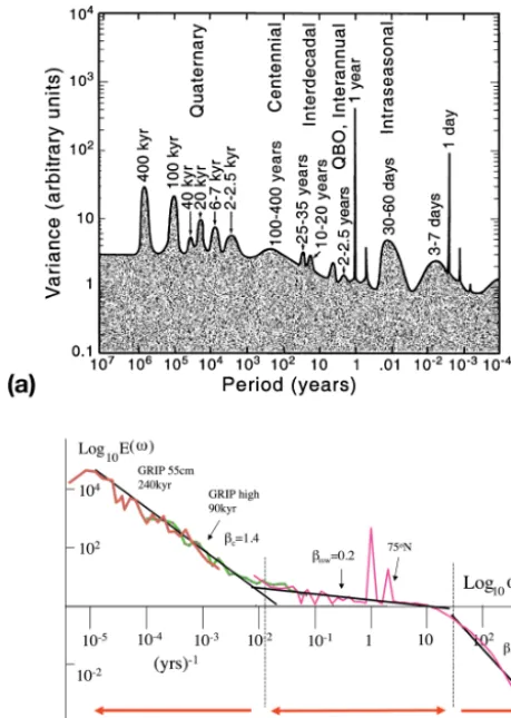
Figure 1. (a)The “background and peaks” paradigm as an artist’s view of climate system variability (figure slightly modified from Mitchell, 1976; see Ghil, 2002, for details). This figure panel is from Dijkstra and Ghil (2005) and reproduced with permission from AGU.(b)A composite temperature spectrum (figure from Lovejoy et al., 2013; see their Fig. 2 for details) to illustrate the “scaling” paradigm.
regimes (Fig. 1b). The “background and peaks” paradigm clearly has a problem with the explanation of the background signal and also regarding the amplitude of the variability on longer than millennial timescales (Lovejoy, 2015). On the other hand, the scaling paradigm needs a better connection to physical processes beyond the weather regime (Franzke et al., 2019). Both paradigms are also limited to temporal variability and do not address spatial patterns associated with the climate system variability.
To understand the results of the observations, i.e., to relate them to elementary well-established physical principles, the observations themselves are in most cases not enough and models are needed. Fortunately, a hierarchy of such models, from conceptual ones (capturing only a few elementary pro-cesses or scales) to global climate models (which are multi-scale and multi-process representations), is available. Tradi-tionally, climate system modeling is seen as an initial value problem. The model equations are integrated in time from
a specific initial condition (or an ensemble of them), and then the transient behavior is analyzed. A subsequent sta-tistical analysis is performed on the results using in general uni- or multivariate statistical methods. Often, parameters in the model are varied to study the sensitivity of the results to physical processes (associated with the parameters) and to determine mechanisms of specific phenomena from the sta-tistical analyses.
Changes in parameters can lead to qualitatively different behavior; for example, oscillatory behavior appears or tran-sitions occur. When relatively strong changes occur under small changes of a parameter, critical conditions associated with so-called tipping behavior may have been crossed.
In particular regarding issues of qualitative changes in model behavior once parameters are varied, there is a com-plementary methodology available from dynamical systems theory, which is targeted to directly compute the asymptotic (long-time) states (attractors) of the model. In the most sim-ple autonomous models (steady forcing), these attractors are fixed points and periodic orbits. Non-autonomous models are studied through pullback attractor analysis (Ghil et al., 2008). Methodology from ergodic theory can be used to study the decay to the attractor of correlations between different ob-servables (Chekroun et al., 2011).
A canonical problem of transition behavior in fluid dynam-ics is the flow between two concentric cylinders of which only the inner cylinder rotates with an angular frequency, the Taylor–Couette flow (Koschmieder, 1993). An overview of the regimes of flow behavior and dynamical systems methodology that can be applied is presented in Fig. 2. Here, the rotation rate of the inner cylinderis used as the main parameter which is changed. In the case of small, numer-ical bifurcation theory can be applied to study the steady states of these models and to determine mechanisms of tran-sition through instabilities. The transient behavior, as shown in time series in Fig. 2, can also be visualized in phase/state space where time is implicit (displaying trajectories). Once is increased, a collective interaction between the differ-ent instabilities can lead to variability which cannot be un-derstood as a single bifurcation. Basically, here the realm of complex systems science is entered, which deals with emer-gent properties due to such collective interactions. For large , eventually a turbulent regime is reached where (actually surprisingly) multiple large-scale statistical steady states can be observed (Huisman et al., 2014).
Figure 2.Sketch of dynamical systems concepts and approaches for the Taylor–Couette flow (as modified from Abraham and Shaw, 1992). Time series, trajectories and the geometrical view of attractors are sketched. Transition behavior at small values ofcan be addressed by bifurcation theory; for large values ofit can be tackled using ergodic theory.
been done so far and what has been learned. This is followed by Sect. 4, where an outlook is given for the role of dynam-ical systems analysis in developing an overarching theory of climate variability.
2 Methodology 2.1 Model hierarchy
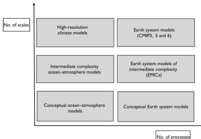
In Dijkstra (2013), I suggested to classify climate models ac-cording to the two traits “scales” and “processes” (Fig. 3). Here the trait “scales” refers to both spatial and temporal scales as there exists a relation between both: on smaller spa-tial scales usually faster processes take place. “Processes” refers to either physical, chemical or biological processes taking place in the different climate subsystems. Models with a limited number of processes and scales are usually referred to as conceptual climate models. Examples are box mod-els of the ocean circulation (Stommel, 1961) and modmod-els of glacial–interglacial cycles (Crucifix, 2012), all formulated by small-dimensional systems of ordinary differential equa-tions. Limiting the number of processes, scales can be added by discretizing the governing partial differential equations spatially up to three dimensions. A higher spatial resolution and inclusion of more processes will give models located in the upper right part of the diagram, so-called Earth system models (ESMs). Between the conceptual models and ESMs are so-called intermediate complexity models which are
spa-tially extended (described by partial differential equations) but with fewer scales and/or processes (Fig. 3).
Any spatially extended climate model consists of a set of conservation laws, which are formulated as a set of coupled partial differential equations, that can be written in general form as (Griffies, 2004)
Mλ ∂u
∂t =Lλu+Nλ(u)+Fλ(u), (1) whereLandMare linear operators,N is a nonlinear opera-tor,uis the state vector,Fcontains the forcing of the system, andλindicates the dependence of the operators on parame-ters. Appropriate boundary and initial conditions have to be added to this set of equations for a well-posed problem.
When Eq. (1) is discretized, eventually a set of differen-tial equations with algebraic constraints arises, which can be written as
Mλ dx
dt =Lλx+Nλ(x)+Fλ(x), (2) wherex∈Rn is the state vector, nits dimension,Mλ is a (often singular) matrix of which every zero row is associated with an algebraic constraint,Lλ is the discretized version of
Lλ, andFλandNλare the finite-dimensional versions of the forcing and the nonlinear operator, respectively.
When noise is added, the evolution of the flow can gener-ally be described by a stochastic differential-algebraic equa-tion of the form
Figure 3.Organization of climate models according to the two model traits: number of processes and number of scales (Dijkstra, 2013).
whereXtis now the stochastic state vector,fλ(Xt)contains the linear and nonlinear processes, and the forcing. The quan-tityWt∈Rnwis a vector ofnw-independent standard Brown-ian motions (Gardiner, 2009) andgλ(Xt)∈Rn×nw. Here, we use the Itô interpretation to represent unresolved processes but the Stratonovich interpretation can also be used (depend-ing on the nature of processes represented).
2.2 Continuation methods
These methods form part of the numerical bifurcation anal-ysis toolbox; here we are restricted to a single parameterλ. Finding steady states of the system (Eq. 2) versusλamounts to solving
fλ(x)=Lλx+Nλ(x)+Fλ(x)=0. (4) The idea of pseudo-arc-length continuation (Keller, 1977; Seydel, 1994) is to parametrize branches of solutions0(s)≡ (x(s), λ(s)) with an arc-length parameters (or an approx-imation of it, thus the term “pseudo”) and choose s as the continuation parameter. An additional equation is obtained by approximating the normalization condition of the tangent
˙
0(s)= x˙(s),λ(s)˙
to the branch0(s), where the dot refers to the derivative with respect tos, with0˙
2
=1. More pre-cisely, for a given solution(x0, λ0), the next solution(x, λ) is required to satisfy the constraint
˙
xT0(x−x0)+ ˙λ0(λ−λ0)−1s=0, (5) where0˙0= x˙0,λ˙0
is the normalized direction vector of the solution family0(s)at(x0, λ0)and1sis an appropriately
small step size. Equation (5) stipulates that the projection of(x, λ)−(x0, λ0)onto(x˙0,λ˙0)has the value1s. Efficient solution methods for high-dimensional systems of the form (Eqs. 4–5) are presented in De Niet et al. (2007) and Thies et al. (2009).
Suppose that the deterministic part of Eq. (3) has a stable fixed pointx∗λ for a given range of parameter values. Then linearization of Eq. (3) around the deterministic steady state yields, withYt=Xt−x∗λ(Kuehn, 2012),
MλdYt=Aλ(x∗λ)Ytdt+Bλ(x∗λ)dWt, (6) where Aλ(x)≡ Dxfλ
(x) is the Jacobian matrix and Bλ(x)=gλ(x).
In the special case thatMλ is a non-singular matrix, the Eq. (6) can be rewritten (dropping the arguments and sub-scripts on the matrices) in Itô form as
dYt=M−1AYtdt+M−1BdWt, (7) which represents ann-dimensional Ornstein–Uhlenbeck pro-cess. The corresponding stationary covariance matrixC is then determined from the generalized Lyapunov equation:
ACMT+MCAT+BBT=0. (8)
3 Main issues
Numerical bifurcation methodology has been mostly applied to dynamical systems with smalln, typicallyn <10, result-ing from conceptual climate models. However, I will focus here solely on results of studies using intermediate complex-ity models with typically n=104–105, because then also spatial information on the bifurcation behavior is obtained.
From elementary bifurcation theory (Guckenheimer and Holmes, 1990) it is known that only four bifurcations can generically occur when a single parameter is varied: the saddle-node bifurcation, the transcritical bifurcation, the pitchfork bifurcation and the Hopf bifurcation. Because the transcritical bifurcation (solution needed for all values of the parameter) and the pitchfork bifurcation (reflection sym-metry needed) require special conditions, the only generic cases are the saddle-node and the Hopf bifurcations. Of these, saddle-node bifurcation only occurs in pairs (because of boundedness of solutions), and hence one often refers to a back-to-back saddle-node bifurcation.
The back-to-back saddle-node bifurcation structure is canonical for tipping points, which we will discuss in Sect. 3.1 below. Although the dynamical system is high-dimensional, the behavior of the system can be dominated by only a few (even only one) positive feedbacks, and hence transitions occur in a low-dimensional space. The Hopf bi-furcation is canonical for the occurrence of spontaneous os-cillatory behavior associated with one eigenmode of the lin-earized dynamical system, which is often referred to as the leading mode. A Hopf bifurcation needs the presence of both positive and negative feedbacks; when only a few dom-inate the dynamical behavior these can be found in high-dimensional systems as discussed in Sect. 3.2. In models where a sequence of Hopf bifurcations occurs, the resulting behavior can in general no longer be described using low-dimensional dynamics. In this case, collective interactions occur and this cannot be captured in a single bifurcation and associated pattern. This case will be discussed in Sect. 3.3 below.
3.1 Tipping points
An overview of possible tipping elements in the Earth’s sys-tem is given in Lenton et al. (2008) and Steffen et al. (2018) and includes the Arctic winter sea ice, the marine ice sheets (MISs), the Amazon rainforest and the Atlantic Meridional Overturning Circulation (AMOC). Several of the associated transitions are thought to be associated with the existence of a multiple equilibrium regime associated with a back-to-back saddle-node structure, in particular the collapse of the AMOC and that of the MIS.
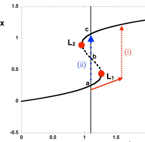
For a back-to-back saddle-node bifurcation there are two transition scenarios possible, called (i) bifurcation tipping and (ii) noise-induced tipping (Ditlevsen and Johnsen, 2010). In case (i) the parameter crosses a value at one of the
saddle-node bifurcations, and in case (ii) a finite amplitude pertur-bation in the state vector causes a transition (even for a fixed value of the parameter). In the non-autonomous case also rate-induced tipping (Ashwin et al., 2012) is possible. For both cases (i) and (ii), it is crucial to determine the extent of the multiple equilibrium regime (Fig 4): this has been investi-gated in detail in spatially extended models for the following problems.
– AMOC. In a substantial number of papers, the bifurcation diagrams for both spatially two- and three-dimensional (intermediate complexity) ocean-only models of the AMOC have been determined (see chap. 6 in Dijkstra, 2005). The most advanced result is for a global ocean model coupled to an energy bal-ance atmospheric model (den Toom et al., 2012), cap-turing ocean–atmosphere feedbacks, where also a back-to-back saddle-node structure was found.
Numerical bifurcation analyses provided the basis for the stability indicator 6=Movs −Movn of the multi-ple equilibrium regime of the AMOC (Huisman et al., 2010). Here, Mov is the AMOC-induced freshwater transport, and the superscripts n and s indicate the north-ern and southnorth-ern boundaries of the Atlantic, respec-tively. Although the central idea was already formu-lated in Rahmstorf (1996) and de Vries and Weber (2005), only bifurcation analysis of high-dimensional discretized ocean models provided more rigorous sup-port for the use of this indicator. Although this stabil-ity indicator has its problems (Gent, 2018) and needs to be extended in a coupled ocean–atmosphere context, it is often used to investigate the stability of the AMOC (Hawkins et al., 2011).
For a spatially two-dimensional ocean-only model, the covariance matrices Cwere determined from solving the Lyapunov equation in Eq. (8) in Baars et al. (2017) for the case of noise in the freshwater forcing. While here it served only to test the new Lyapunov equa-tion solver (RAILS), the methodology was extended re-cently to compute (noise-induced) transition probabil-ities of the AMOC and to relate that probability to the stability indicator6(Castellana et al., 2019). Such tran-sitions are thought to be involved in the Dansgaard– Oeschger (DO) events (Ditlevsen and Johnsen, 2010). – MIS. The explicit computation of the bifurcation
dif-Figure 4.The canonical bifurcation diagram with the back-to-back saddle node indicating two stable states (a, c) and an unstable state (b). Bifurcation tipping occurs when the parameterλcrosses the value atL1orL2. Noise-induced tipping (e.g., from state a to
state c) can occur through a perturbation in the state vector (for fixed
λ).
ferent model studies (Gomez et al., 2010), the precise mechanism could be deduced from the bifurcation dia-gram shift (Mulder et al., 2018). For a stochastic MIS model, the covariance matricesCwere determined for each stable state in Mulder et al. (2018). Typical noise in the accumulation leads to grounding line variations on the order of 1000 m, while for sea level noise this is about 100 m. In the multiple equilibrium regime, the study of the transition probabilities indicated that, for both noise types, it is more likely to jump from a large ice sheet state to a small ice sheet state than vice versa. In high-dimensional climate models, also so-called edge states or Melancholy states have been computed, for exam-ple in a couexam-pled atmospheric sea-ice model investigating ice-covered/ice-free multi-stability (Lucarini and Bódai, 2017). This edge state is a saddle embedded in the boundary be-tween the two basins of attraction of the stable climate states. 3.2 Patterns of sea surface temperature (SST)
variability
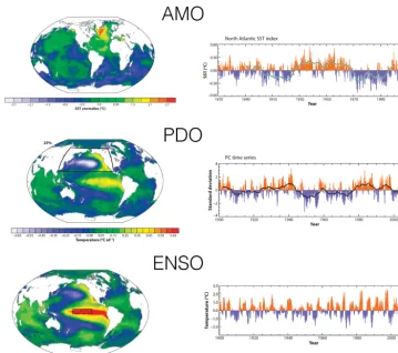
It is remarkable that on interannual-to-multidecadal timescales the variability in sea surface temperature is organized in large-scale patterns (Fig. 5). These patterns have been detected by using multi-variate analysis on long data sets, such as the HadISST, for example through principal component analysis where the patterns are then
contained in the empirical orthogonal functions (EOFs). Well-known and much-studied patterns are those of the El Niño–Southern Oscillation (ENSO), the Atlantic Mul-tidecadal Oscillation (Enfield et al., 2001) and the Pacific Decadal Oscillation (PDO) (Mantua et al., 1997), as shown in Fig. 5.
Numerical bifurcation analysis has been applied to several spatially extended models, in particular ENSO, PDO and the AMO.
– ENSO. The cornerstone intermediate complexity model is the Zebiak–Cane (ZC) model of which the behavior has been extensively analyzed (Zebiak and Cane, 1987). Numerical bifurcation analysis of different versions of the ZC model were performed (see chap. 7 in Dijkstra, 2005), and in each of them a Hopf bifurcation occurs once the coupling strength between the equatorial ocean and atmosphere crosses a critical value. The period of the leading mode is in the interannual range and deter-mined by basin modes, just as in the recharge–discharge oscillator model (Jin, 1997). The spatial pattern of the leading mode is localized into the cold tongue region of the mean (steady) state and shares many similarities with the first EOF from observations.
– AMO. One of the intermediate complexity models which has been used is a spatially three-dimensional model of the North Atlantic (see chap. 8 in Dijkstra, 2013). The mean (steady) state is generated by a hori-zontal atmospheric surface buoyancy field which drives a meridional overturning circulation in the ocean model. Numerical bifurcation analysis of this model has shown that the background state destabilizes through a multi-decadal leading mode, and hence a Hopf bifurcation oc-curs. The timescale of the leading mode can be linked to the basin crossing time of temperature anomalies, and its spatial pattern shares many features with the ob-served pattern (Kushnir, 1994) when a representation of the continents is considered. The variability can be eas-ily excited through noise in the heat flux, even when the leading mode is decaying in the deterministic case (see chap. 8 in Dijkstra, 2013).
Figure 5.Overview of patterns of climate variability (AMO, PDO and ENSO) as determined in Deser et al. (2010) with accompanying time series.
My interpretation of these results is that several of these SST patterns (but not all) appear through a normal mode which destabilizes the mean state through positive feedbacks; the presence of negative feedbacks causes the oscillatory be-havior. In this case, the associated Hopf bifurcation (of a spa-tially extended model) provides both the dominant timescale of variability and its spatial pattern. The elegant structure of leading modes in ocean models and the ZC model was pre-sented in Dijkstra (2016). The key to why normal modes can be dominant in this variability may be that the nonlinearity in these models is rather weak (it involves advection of heat/salt and not of momentum). Hence the mean state is not modified (rectified) much due to the nonlinear interactions (contrary to the processes shown in the next section).
3.3 Collective interactions and emergent behavior
In the previous two subsections climate system variability phenomena were attributed to low-order dynamics. However, there are many phenomena which are intrinsically caused by the collective interaction of multiple instabilities. Clearly, the role of numerical bifurcation theory becomes quite limited
in determining the behavior of these (in general) chaotic dy-namical systems; I briefly describe below two examples.
– Ocean western boundary current variability (WBC). In pure wind-driven barotropic shallow-water models, the bifurcation structure consists of an imperfect pitchfork bifurcation followed by several Hopf bifurcations con-taining two types of modes: Rossby modes and so-called gyre modes. These gyre modes are eventually responsible for homoclinic orbits which lead to ultra-low-frequency behavior (see chap. 5 in Dijkstra, 2005). When another layer is added, baroclinic instabilities lead to a range of normal modes (Simonnet et al., 2003) which all destabilize. Hence the eventual emergent be-havior is induced by their collective interactions. Such behavior can lead to low-frequency behavior in the sta-tistical steady state which has been referred to as the turbulent oscillator (Berloff et al., 2007).
a collective interaction and low-frequency variability emerges in the statistical equilibrium state (Crommelin et al., 2004). Approaches to understand the dynamics on the attractor have been proposed through transfer oper-ator methods (Tantet et al., 2015).
The cases briefly described above are examples of strongly nonlinear systems, where the nonlinearities occur in the mo-mentum advection and where the mean state is strongly modified through rectification. Of course, there are many more examples of such geophysical systems, in particular on timescales up to interannual both in the ocean (internal waves) and the atmosphere (weather).
4 Discussion and outlook
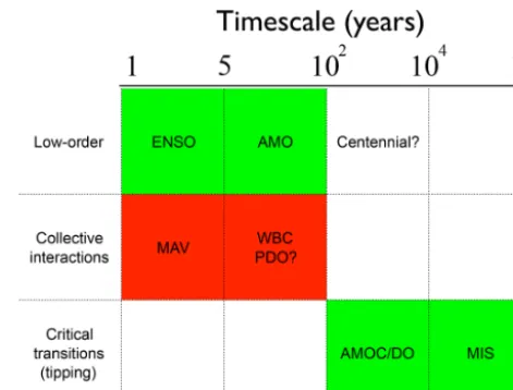
In this paper, I have given a short overview of results of stud-ies where continuation methods were applied to spatially ex-tended climate models. My interpretation of these results is that there are climate variability phenomena that can be at-tributed to low-order behavior; only one or a few spatial pat-terns are involved, associated with dominant feedbacks. Sev-eral of these studies have shown that successive instability behavior can also occur. This leads to a collective interaction between patterns that is eventually responsible for emergent variability in climate models. A summary of the different phenomena based on this distinction is provided in Fig. 6, with low-order phenomena (ENSO, AMO), emergent phe-nomena due to collective interactions (WBC, MAV) and tip-ping behavior (AMOC/DO, MIS). With this information, I now come back to the two paradigms of climate variability, as mentioned in the introduction.
This first challenge I see is to better understand processes behind the background variability which is “red noise like” in Mitchell (1976) and encompasses different regimes in Love-joy et al. (2013). Franzke et al. (2019) describe the differ-ent ways (multifractal cascading processes, state-dependdiffer-ent noise, etc.) of how scaling behavior can appear in time series. To connect scaling behavior to clear physical processes, one idea would be to identify at each timescale range the “slow” passive component in the climate system and the “fast” forc-ing it receives. For example, for SST variability the Hassel-mann (1976) model of an ocean mixed layer forced with a rapidly fluctuating atmospheric heat flux identifies such com-ponents, leading to a red noise background. However, when another variable is considered, such as sea surface height, then the background model is an ocean thermocline layer forced with noisy wind-stress forcing, leading to a corre-lated additive–multiplicative (CAM) noise model (Sardesh-mukh and Sura, 2009; Castellana et al., 2018). In the “climate regime” of Lovejoy et al. (2013), an appropriate model could be a marine ice sheet forced with rapidly fluctuating accu-mulation noise or sea level noise (Mulder et al., 2018), also leading to CAM noise. This would give power law spectral behavior (in the proxy record), being indeed very different
Figure 6.Summary of what has been learned from dynamical sys-tems analysis of spatially extended climate models, based on the distinction of low-order phenomena, emergent phenomena through collective interactions and critical transitions. The “hope” is that mechanisms of the phenomena in the green boxes can be deter-mined from numerical bifurcation analysis of intermediate com-plexity climate models.
from the picture of Mitchell (1976). The slope changes of the different regimes as in Lovejoy et al. (2013) could then maybe be related to a change in slow component in the cli-mate system determining this background signal.
Once the physics of this background are clear, the next challenge is to attribute spatial patterns which rise above it to specific instabilities. Several spatial patterns of SST vari-ability are robust over the model hierarchy. I would inter-pret this to indicate that these spatial patterns, such as ENSO and the AMO, are due to a single-mode destabilization of the background induced by dominant large-scale feedbacks. These spatial patterns can already be captured in detail in intermediate complexity models, such as the ZC model for ENSO. Capturing the temporal variability involves repre-sentation of small-scale processes (noise) and possibly non-normal growth (Penland and Sardeshmukh, 1995; Farrell and Ioannou, 1996; Tziperman et al., 2008), and one may need more detailed models than intermediate complexity models. Another case where a low-order explanation may be appro-priate is centennial variability. The timescale here arises by buoyancy anomalies which propagate over the AMOC loop (also called overturning modes and loop oscillations). These can be excited in this model by applying noise, e.g., in the freshwater flux or in the heat flux (Dijkstra and von der Heydt, 2017).
Current, where it is known that the interactions of the barotropic instabilities of the current and the (baroclinic) mesoscale eddy field are important (Qiu and Chen, 2005). Such collective interactions may eventually also be needed to explain the PDO. Furthermore, analysis of high-resolution (near-eddy resolving) ocean model has indicated that a new type of multidecadal variability emerges through a collec-tive interaction, the Southern Ocean mode. A Lorenz type energy analysis has indicated (Jüling et al., 2019) that eddy– mean-flow interaction is crucial for the existence of this type of variability. Also in this case, there is no single (normal) mode of variability which determines the dominant time and spatial pattern.
Apart from the internal variability introduced by single normal (oscillatory) modes and collective phenomena, also clear large-scale tipping phenomena (in the sense of critical transitions) can affect climate variability. The canonical be-havior is a back-to-back saddle-node bifurcation appearing generically in conceptual models. It was shown here that for models of the AMOC and MIS, indeed such bifurcation havior is found in high-dimensional models. Transition be-havior hence may occur when critical conditions are crossed or through noise in the multiple equilibrium regime. A third challenge I see is to show that such transitions remain robust once small-scale processes are included; work in this direc-tion has been initiated (Lucarini and Bódai, 2017).
All of the results of continuation methods described above were obtained under stationary forcing and this seems dis-joint from the real climate system, which is obviously forced by a non-stationary insolation component (on diurnal, sea-sonal and orbital timescales). For the present-day climate system, there is also the non-stationary anthropogenic com-ponent of climate change. A fourth challenge is to understand the relevance of these diurnal and seasonal non-stationary pe-riodic components in natural internal variability on longer timescales. While one may argue that they are irrelevant and are averaged out, few detailed results are available. Proba-bly only on interannual timescales can there be an interaction between the seasonal cycle and internal variability, for exam-ple, with the ENSO mode (due to nonlinear resonances). On very large timescales, however, certainly the non-stationary orbital forcing is crucial for the observed variability such as glacial cycles. The modification of natural variability under climate forcing is of course also a challenging issue.
Has the end point been reached of the models for which bifurcation analysis can be applied? Since starting with this endeavor in the early 1990s, I have been repeatedly asked this question. When we showed results for spatially two-dimensional ocean models, we were asked if we could do this for three-dimensional models. When we did, the ques-tion was on the applicaques-tion to ocean–atmosphere models. Al-though there are certainly still interesting details to be inves-tigated in the ocean-only context, I think the main challenge with these models is to develop theory for internal variability in the geological past (Zachos et al., 2001). In the last few
years my group has turned to develop techniques to incorpo-rate sea ice and land ice and to be able to change the geome-try of the ocean basin during the continuation (Mulder et al., 2017). With a carbon cycle model still to be implemented, I think that the resulting methodology will be suited to tackle what processes determined the background states in the past and which variability can possibly be attributed to low-order dynamics. It will also be possible to investigate explicit bi-furcation behavior arising from carbon-cycle feedbacks.
Competing interests. The author declares that there is no conflict of interest.
Special issue statement. This article is part of the special issue “Centennial issue on nonlinear geophysics: accomplishments of the past, challenges of the future”. It is not associated with a conference.
Acknowledgements. The author thanks his “partner in crime”, Fred W. Wubs (University of Groningen, the Netherlands), for the (now
∼25 years) long and very fruitful (still very active) collabora-tion regarding the applicacollabora-tion of numerical bifurcacollabora-tion analysis in high-dimensional stochastic dynamical systems arising from cli-mate models. I also thank the many contributions from the PhDs and postdocs who have worked on our joint projects, in particular the current ones: Erik Mulder, Sven Baars and Daniele Castellana. I also thank Andrew Keane and Bernd Krauskopf (University of Auckland, NZ) for organizing a session at the SIAM conference on Dynamical Systems (May 2019), where the ideas in this paper could be presented.
Financial support. This work was sponsored by the Netherlands Earth System Science Centre (NESSC), financially supported by the Ministry of Education, Culture and Science (OCW (grant no. 024.002.001)).
Review statement. This paper was edited by Ana M. Mancho and reviewed by two anonymous referees.
References
Abraham, R. and Shaw, C.: Dynamics: The Geometry of Behavior, Addison-Wesley, Redwood City, California, USA, 1992. Ashwin, P., Wieczorek, S., Vitolo, R., and Cox, P.: Tipping points in
open systems: bifurcation, noise-induced and rate-dependent ex-amples in the climate system, Philos. T. Roy. Soc. A, 370, 1166– 1184, 2012.
Berloff, P. S., Hogg, A. M., and Dewar, W. K.: The turbulent oscilla-tor: a mechanism of low-frequency variability of the wind-driven ocean gyres, J. Phys. Oceanogr., 37, 2362–2386, 2007.
Castellana, D., Wubs, F., and Dijkstra, H.: A statisti-cal significance test for sea-level variability, Dynam-ics and Statistics of the Climate System, 3, dzy008, https://doi.org/10.1093/climsys/dzy008, 2018.
Castellana, D., Baars, S., Wubs, F., and Dijkstra, H.: Transition Probabilities of Noise-induced AMOC Transitions, Nature Sci-entific Reports, submitted, 2019.
Chekroun, M. D., Simonnet, E., and Ghil, M.: Stochastic climate dynamics: Random attractors and time-dependent invariant mea-sures, Physica D, 240, 1685–1700, 2011.
Clement, A. C. and Peterson, L. C.: Mechanisms of abrupt climate change of the last glacial period, Rev. Geophys., 46, RG4002, https://doi.org/10.1029/2006RG000204., 2008.
Crommelin, D.: Regime transitions and heteroclinic connections in a barotropic atmosphere, J. Atmos. Sci., 60, 229–246, 2003. Crommelin, D., Opsteegh, J., and Verhulst, F.: A mechanism for
at-mospheric regime behavior, J. Atmos. Sci., 61, 1406–1419, 2004. Crucifix, M.: Oscillators and relaxation phenomena in Pleistocene
climate theory, Philos. T. Roy. Soc. A, 370, 1140–1165, 2012. De Niet, A. C., Wubs, F., Terwisscha van Scheltinga, A. D., and
Dijkstra, H. A.: A tailored preconditioner for high-resolution im-plicit ocean models, J. Comput. Phys., 277, 654–679, 2007. den Toom, M. d., Dijkstra, H. A., Cimatoribus, A. A., and Drijfhout,
S. S.: Effect of Atmospheric Feedbacks on the Stability of the At-lantic Meridional Overturning Circulation, J. Climate, 25, 4081– 4096, 2012.
Deser, C., Alexander, M. a., Xie, S.-P., and Phillips, A. S.: Sea Sur-face Temperature Variability: Patterns and Mechanisms, Annu. Rev. Mar. Sci., 2, 115–143, 2010.
de Vries, P. and Weber, S. L.: The Atlantic freshwater budget as a diagnostic for the existence of a stable shut down of the merid-ional overturning circulation, Geophys. Res. Lett., 32, L09606, https://doi.org/10.1029/2004GL021450, 2005.
Dijkstra, H.: A Normal Mode Perspective of Intrinsic Ocean-Climate Variability, Annu. Rev. Fluid Mech., 48, 341–363, 2016. Dijkstra, H. A.: Nonlinear Physical Oceanography: A Dynamical Systems Approach to the Large Scale Ocean Circulation and El Niño, 2nd revised and enlarged edn., Springer, New York, 532 pp., 2005.
Dijkstra, H. A.: Nonlinear Climate Dynamics, Cambridge Univer-sity Press, Cambridge, UK, 2013.
Dijkstra, H. A. and Ghil, M.: Low-frequency variability of the large-scale ocean circulation: A dynamical systems approach, Rev. Geophys., 43, RG3002, https://doi.org/10.1029/2002RG000122, 2005.
Dijkstra, H. A. and von der Heydt, A. S.: Basic mechanisms of cen-tennial climate variability, Past Global Changes Magazine, 25, 150–151, 2017.
Ditlevsen, P. D. and Johnsen, S. J.: Tipping points: Early warn-ing and wishful thinkwarn-ing, Geophys. Res. Lett., 37, L19703, https://doi.org/10.1029/2010GL044486, 2010.
Enfield, D. B., Mestas-Nunes, A. M., and Trimble, P.: The Atlantic multidecadal oscillation and its relation to rainfall and river flows in the continental US, Geophys. Res. Lett., 28, 2077–2080, 2001. Farrell, B. F. and Ioannou, P. J.: Generalized stability theory: Part I:
Autnomous operators, J. Atmos. Sci., 53, 2025–2040, 1996.
Franzke, C. L. E., Barbosa, S., Blender, R., Fredriksen, H., Laep-ple, T., Lambert, F., Nilsen, T., Rypdal T., Rypdal, M., Scotto, M., Vannitsem, S., Watkins, N., Yang, L., and Yuan, N.: The Structure of Climate Variability Across Scales, Rev. Geophys., submitted, 2019.
Gardiner, C.: Stochastic Methods: A Handbook for the Natural and Social Sciences, Springer, New York, 2009.
Gent, P. R.: A commentary on the Atlantic meridional overturning circulation stability in climate models, Ocean Model., 122, 57– 66, https://doi.org/10.1016/j.ocemod.2017.12.006, 2018. Ghil, M.: Natural Climate Variability, in: Encyclopedia of Global
Environmental Change, volume 1, edited by: Munn, T., Mac-Cracken, M. C., and Perry, J. S., Wiley, Hoboken, New Jersey, 2002.
Ghil, M., Chekroun, M., and Simonnet, E.: Climate dynamics and fluid mechanics: Natural variability and related uncertainties, Physica D, 237, 2111–2126, 2008.
Gomez, N., Mitrovica, J. X., Huybers, P., and Clark, P. U.: Sea level as a stabilizing factor for marine-ice-sheet grounding lines, Nat. Geosci., 3, 850–853, 2010.
Griffies, S. M.: Fundamentals of ocean-climate models, Princeton University Press, Princeton, USA, 2004.
Guckenheimer, J. and Holmes, P.: Nonlinear Oscillations, Dynami-cal Systems and Bifurcations of Vector Fields, 2e edn., Springer-Verlag, Berlin/Heidelberg, 1990.
Hasselmann, K.: Stochastic climate models. I: Theory, Tellus, 28, 473–485, 1976.
Hawkins, E., Smith, R. S., Allison, L. C., Gregory, J. M., Woollings, T. J., Pohlmann, H., and De Cuevas, B.: Bistability of the At-lantic overturning circulation in a global climate model and links to ocean freshwater transport, Geophys. Res. Lett., 38, L10605, https://doi.org/10.1029/2011GL047208, 2011.
Huisman, S. E., den Toom, M., Dijkstra, H. A., and Drijfhout, S.: An Indicator of the Multiple Equilibria Regime of the At-lantic Meridional Overturning Circulation, J. Phys. Oceanogr., 40, 551–567, 2010.
Huisman, S. G., van der Veen, R. C. A., Sun, C., and Lohse, D.: Multiple states in highly turbulent Taylor-Couette flow, Nat. Commun., 5, 3820, https://doi.org/10.1038/ncomms4820, 2014. Jin, F.-F.: An equatorial recharge paradigm for ENSO. I: Conceptual
Model, J. Atmos. Sci., 54, 811–829, 1997.
Jüling, A., Viebahn, J. P., Drijfhout, S. S., and Dijkstra, H. A.: En-ergetics of the Southern Ocean Mode, J. Geophys. Res.-Oceans, 123, 9283–9304, 2019.
Keller, H. B.: Numerical solution of bifurcation and nonlinear eigenvalue problems, in: Applications of Bifurcation Theory, edited by: Rabinowitz, P. H., Academic Press, New York, USA, 1977.
Koschmieder, E. L.: Bénard Cells and Taylor Vortices, Cambridge University Press, Cambridge, UK, 1993.
Kuehn, C.: Deterministic continuation of stochastic metastable equilibria via Lyapunov equations and ellipsoids, SIAM J. Sci. Comput., 34, A1635–A1658, 2012.
Kushnir, Y.: Interdecadal variations in North Atlantic sea sur-face temperature and associated atmospheric conditions, J. Phys. Oceanogr., 7, 141–157, 1994.
edited by: Moreau, R., Gauthier-Villars, Paris, J. Méc. Théor. Appl., 45–82, 1983.
Lenton, T. M., Held, H., Kriegler, E., Hall, J. W., Lucht, W., Rahm-storf, S., and Schellnhuber, H. J.: Tipping elements in the Earth’s climate system, P. Natl. Acad. Sci. USA, 105, 1786–93, 2008. Lovejoy, S.: A voyage through scales, a missing quadrillion and
why the climate is not what you expect, Clim. Dynam., 44, 3187– 3210, 2015.
Lovejoy, S. and Schertzer, D.: The weather and climate: emer-gent laws and multifractal cascades, Cambridge University Press, First Cambridge Mathematical Library Edition, Cambridge, UK, 2013.
Lovejoy, S., Schertzer, D., and Varon, D.: Do GCMs predict the climate ... or macroweather?, Earth Syst. Dynam., 4, 439–454, https://doi.org/10.5194/esd-4-439-2013, 2013.
Lucarini, V. and Bódai, T.: Edge states in the climate system: ex-ploring global instabilities and critical transitions, Nonlinearity, 30, R32, https://doi.org/10.1088/1361-6544/aa6b11, 2017. Mantua, N. J., Hare, S., Zhang, Y., Wallace, J. M., and Francis,
R. C.: A Pacific interdecadal climate oscillation with impacts on salmon production, B. Am. Meteor. Soc., 78, 1069–1079, 1997. Mitchell, J. M.: An overview of climate variability and its causal
mechanisms, Quaternary Res., 6, 481–493, 1976.
Mulder, T. E., Baatsen, M. L. J., Wubs, F. W., and Dijkstra, H. A.: Efficient computation of past global ocean circulation patterns using continuation in paleobathymetry, Ocean Model., 115, 77– 85, 2017.
Mulder, T. E., Baars, S., Wubs, F. W., and Dijkstra, H. A.: Stochastic marine ice sheet variability, J. Fluid Mech., 843, 748–777, 2018. Newman, M., Alexander, M. A., Ault, T. R., Cobb, K. M., Deser, C., Di Lorenzo, E., Mantua, N. J., Miller, A. J., Minobe, S., Naka-mura, H., Schneider, N., Vimont, D. J., Phillips, A. S., Scott, J. D., and Smith, C. A.: The Pacific Decadal Oscillation, Revis-ited, J. Climate, 29, 4399–4427, 2016.
Penland, C. and Sardeshmukh, P. D.: The optimal growth of tropi-cal sea surface temperature anomalies, J. Climate, 8, 1999–2024, 1995.
Philander, S. G. H.: El Niño and the Southern Oscillation, Academic Press, New York, 1990.
Qiu, B. and Chen, S.: Variability of the Kuroshio Extension Jet, Recirculation Gyre and Mesocale Eddies on decadal time scales, J. Phys. Oceanogr., 35, 2090–2103, 2005.
Rahmstorf, S.: On the freshwater forcing and transport of the At-lantic thermohaline circulation, Clim. Dynam., 12, 799–811, 1996.
Sardeshmukh, P. D. and Sura, P.: Reconciling Non-Gaussian Cli-mate Statistics with Linear Dynamics, J. CliCli-mate, 22, 1193– 1207, 2009.
Schoof, C.: Ice sheet grounding line dynamics: Steady states, stability, and hysteresis, J. Geophys. Res., 112, F03S28, https://doi.org/10.1029/2006JF000664, 2007.
Seydel, R.: Practical Bifurcation and Stability Analysis: From Equi-librium to Chaos, Springer-Verlag, New York, USA, 1994. Simonnet, E., Ghil, M., Ide, K., Temam, R., and Wang, S.:
Low-frequency variability in shallow-water models of the wind-driven ocean circulation. Part I: Steady-state solutions, J. Phys. Oceanogr., 33, 712–728, 2003.
Steffen, W., Rockström, J., Richardson, K., Lenton, T. M., Folke, C., Liverman, D., Summerhayes, C. P., Barnosky, A. D., Cornell, S. E., Crucifix, M., Donges, J. F., Fetzer, I., Lade, S. J., Scheffer, M., Winkelmann, R., and Schellnhuber, H. J.: Trajectories of the Earth System in the Anthropocene, P. Natl. Acad. Sci. USA, 115, 8252–8259, 2018.
Stommel, H.: Thermohaline convection with two stable regimes of flow, Tellus, 2, 244–230, 1961.
Tantet, A., van der Burgt, F. R., and Dijkstra, H. A.: An early warn-ing indicator for atmospheric blockwarn-ing events uswarn-ing transfer oper-ators, Chaos: An Interdisciplinary Journal of Nonlinear Science, 25, 036406, https://doi.org/10.1063/1.4908174, 2015.
Thies, J., Wubs, F., and Dijkstra, H. A.: Bifurcation analysis of 3D ocean flows using a parallel fully-implicit ocean model, Ocean Model., 30, 287–297, 2009.
Tziperman, E., Zanna, L., and Penland, C.: Nonnormal Thermo-haline Circulation Dynamics in a Coupled Ocean–Atmosphere GCM, J. Phys. Oceanogr., 38, 588–604, 2008.
von der Heydt, A. and Dijkstra, H. A.: Localization of multidecadal variability: I. Cross equatorial transport and interbasin exchange, J. Phys. Oceanogr., 37, 2401–2414, 2007.
Zachos, J., Pagani, M., Sloan, L., Thomas, E., and Billups, K.: Trends, Rhythms, and Aberrations in Global Climate 65 Ma to Present, Science, 292, 686–693, 2001.