PREDICTION AND CLASSIFICATION
OF THUNDERSTORMS USING
ARTIFICIAL NEURAL NETWORK
S.MAHESH ANAD
Assistant. Professor (Senior), DSP/ISP Division, School of Electrical Sciences Vellore Institute of Technology University, Vellore-632014, INDIA.
ANSUPA DASH
Under Graduate Telecommunication Engineering Student, School of Electrical Sciences Vellore Institute of Technology University, Vellore-632014, INDIA
M.S.JAGADEESH KUMAR
Assistant. Professor (Senior), Applied Mathematics Division, School of Science and Humanities Vellore Institute of Technology University, Vellore-632014, INDIA
AMIT KESARKAR
Scientist-SD, National Atmospheric Research Laboratory, Gadanki, INDIA
Abstract: - Natural calamities cause heavy destruction to both life and property. Prediction of such calamities well in advance is inevitable. Prediction and classification of thunderstorms using Artificial Neural Network (ANN) is presented in this paper. The Numerical Weather Prediction (NWP) models used today suffer from course resolution and inaccuracy. Two geographical locations are considered for our study namely, Paradeep in the west cost of India and Wollemi National Park, New South Wales, (Australia). ANN has designed to forecasts the occurrence of thunderstorm in these regions. Input parameter selection is very critical in ANN design, Eight input parameters were identified to train the network. The output nodes clearly classifies the days with and without thunderstorms, thus successfully predicting thunderstorm activity in the specified regions.
.
Keywords: Artificial Neural Network (ANN), Back Propagation Network (BPN), Thunderstorm Prediction, GRIB, Best Lifted Index, Numerical Weather Prediction (NWP).
1. Introduction
Use of ANN to forecast thunderstorm is order of the day and a few literatures shows successful implementationof predicting convective initiation. ANN is considered to be a form of Artificial Intelligence which has high ability to model non-linear relationships. In this paper, we are presenting the preliminary results obtained in prediction of thunderstorm in two geographical locations Paradeep, Orissa (India) and Wollemi National Park, New South Wales, (Australia). The data has taken from Indian Meteorological Department’s Gridded Binary (GRIB) archive data. Each GRIB file is composed of a series of GRIB records. One GRIB record holds the gridded data for one parameter at one time and at one level. GRID data was decoded using MatLab 7.0 Toolbox. The decoding of GRIB data enabled the access of 234 numbers of parameters. Extraction of the required data from the resulting data after decoding has done to prevent interference of one parameter with another. From the whole 234 parameters, 8 atmospheric parameters such as Best Lifted Index, K- Index, Moisture, amount of Precipitable water, Precipitation rate, relative humidity, U (zonal) component of wind and V (meridional) component of wind were finalised after quantitative analysis. The designed Back Propagation Network (BPN) successfully classifies the data with and without thunderstorm.
2 Methodology
2.1. Data Preparation
The eight input parameters are selected based on how much they change in a state of thunderstorm occurrence as compared to a normal weather day. The following are the parameters and associated justifications.
2.1.1. Lifted Index (LI)
The Lifted Index is the temperature difference between an air parcel lifted adiabatically Tp(p) and the temperature of the environment Te(p) at a given pressure height in the troposphere (lowest layer where most weather occurs) of the atmosphere, usually 500 hPa (mb). When the value is positive, the atmosphere (at the respective height) is stable and when the value is negative, the atmosphere is unstable.
2.1.2. K-Index
The K-index quantifies disturbances in the horizontal component of earth's magnetic field with an integer in the range 0-9 with 1 being calm and 5 or more indicating a geomagnetic storm. It is derived from the maximum fluctuations of horizontal components observed on a magnetometer during a three-hour interval.So, The KI (K Index) is an index used to assess convective potential. The KI is combination of the Vertical Totals (VT) and lower tropospheric moisture characteristics. The VT is the temperature difference between 850 and 500 mb while the moisture parameters are the 850 mb dewpoint and 700 mb dewpoint depression.A high 850 mb dewpoint and a low 700 mb dewpoint depression at the same time indicates there is a deep layer of warm and moist air in the lower to middle troposphere. This is very beneficial to producing instability, especially when the VT is high.
2.1.3. Moisture
Moisture generally refers to the presence of water, often in trace amounts. It is also used to refer to any type of precipitation. Moisture is an absolute essential in our atmosphere. It appears in three forms: gas (humidity), liquid (precipitation), and solid (ice and snow). Precipitation occurs in clouds when rapid condensation takes place. The fallen moisture returns to the oceans, rivers and streams as runoff and ground water where it evaporates again. This recycling of moisture is the hydrologic cycle. Water vapour is the invisible source of clouds and rain and is also a form of heat transfer. Clouds develop when water vapour attaches itself to microscopic matter called nuclei. The moisture holding capacity of air varies with temperature. If there is no change in the total moisture content during a 24 hour period, relative humidity will increase at night. The highest readings occur about sunrise which explains damp lawns and fogged car windows. Relative humidity decreases as the day heats up because warm air has a greater capacity to contain moisture than cold air.
2.1.4. Amount of Precipitable water
Precipitable water (measured in millimeters or inches) is the amount of water in a column of the atmosphere. The Precipitable water value is the depth that would be achieved if all the water in that column were precipitated as rain. Data can be viewed on a Lifted-K index. The numbers represent inches of water as mentioned above for a geographical location. Thus Precipitable water is the amount of liquid precipitation that would result if all the water vapour in a column of air was condensed. The precipitable water value is an indicator of the amount of moisture in the air between the surface and 500mb (18,000ft).
2.1.5. Precipitation rate
It is defined as the rate, expressed in inches per hour, at which water is applied to the surface of a field.
It is defined as the ratio of the partial pressure of water vapour in a gaseous mixture of air and water vapour to the saturated vapour pressure of water at a given temperature.
2.1.7. U – component of wind
The u component of wind gives the direction of wind flow in a horizontal plane. Strong wind can trigger convection. Thus this parameter is very important while dealing with a thunderstorm. The component of wind flowing in a west to east direction of the horizontal plane of an area is referred to as u component of wind.
2.1.8. V- component of wind
The v component of wind gives the direction of wind flow in a horizontal plane. Strong wind can trigger convection. Thus this parameter is very important while dealing with a thunderstorm. The component of wind flowing in a north to south direction of the horizontal plane of an area is referred to as v component of wind.
2.2. Pre-processing of data
Each input node of neural network consists of an array of different atmospheric parameter values at a different time period. The decoding of NWP data led to the access of the data for the entire globe. So, selection of a particular area for consideration for prediction purpose was done. Paradeep, Orissa (India) with Latitude (115- 125) and Longitude ( 280 - 290), Wollemi National Park, New South Wales (Australia) with Latitude (52 – 62) and Longitude ( 326 – 336) were considered for this study. An appropriate grid of size 11o X 11o is fixed based on the latitude and longitude of the desired location. For each parameter, the two dimensional data is converted to one dimensional data 1 X 11 by taking average. Similarly all different eight parameters were extracted and arranged to form a single array of size 1 X 88. The NWP data was considered in an interval of 12 hours over a period of six days. Then the size of the input dataset is 12 X 88. Afterwards, each input parameters were normalized to have the values between -1 to 1 to improve the output of the ANN.
2.3. Artificial Neural Network design
ANN architecture for our design is a feed-forward, supervised, multilayer perceptron network with two layers, with one hidden layer and an output layer trained with back propagation algorithm. The ANN model for this study was developed, trained and tested using MatLab 7.0. The input layer of ANN consists of twelve input nodes (since, 12 hour data for consecutive 6 days were taken). Each input node has an array of 1 X 88 values derived from eight atmospheric parameters. Thus a 12 X 88 dataset is fed as input to the network. For a Multi Layer Perceptron (MLP) with only one hidden layer, Gaussian hills and valleys requires a large number of hidden units to approximate well. Thus the network has designed for single hidden layer. If there are too many hidden units then it may result in low training error but still have high generalization error due to over fitting and high variance. A rule of thumb is for the size of hidden layer to be somewhere between the input layer size and output layer size. The number of hidden layer nodes selected for our design is 9. Each layer was activated by sigmoidal activation function. The design is depicted in the fig.1. The ANN model requires a full input set. A screening of the input and target data is performed once the forecast time and geographical area is selected.
Fig.1.Architecture of Proposed Design
3. Results And Discussion
The designed neural network has implemented according to the proposed architecture. It has trained and tested using different weather data. The weights and bias were updated with each iteration. It was obviously found that error minimized drastically with increase in number of iterations as shown in fig.2 A comparative analysis of error with various levels of iterations also shown in fig 3 and fig 4. As the iterations approaches towards 45000, the error approaches to 0.005.
Fig.2 Error Analysis for 29, Oct 1999, 00hrs data
Fig.4 Error Analysis for various levels of iterations with no thunderstorm data
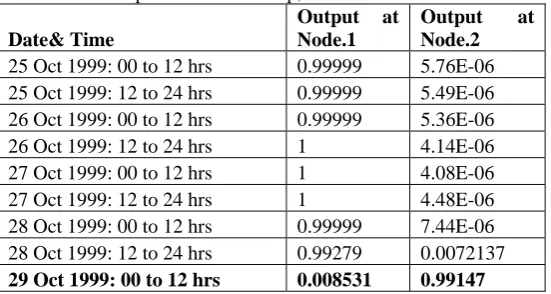
After training the ANN with thunderstorm and non-thunderstorm data, the testing part was carried out. It was observed that the output nodes gave significant distinct result for thunderstorm and non-thunderstorm days. Table I and Table II shows the ANN classification for the Paradeep and New South Wales regions.
Table 1 shows the thunderstorm occurrence is correctly predicted on 29th October, 1999 in the region of Paradeep, Orissa, India and Table 2 shows the correct prediction on 6th December 2000 at Wollemi National Park, New South Wales, Australia.
Table I: ANN output for the Paradeep, Orissa
Date& Time
Output at Node.1
Output at Node.2
25 Oct 1999: 00 to 12 hrs 0.99999 5.76E-06 25 Oct 1999: 12 to 24 hrs 0.99999 5.49E-06 26 Oct 1999: 00 to 12 hrs 0.99999 5.36E-06 26 Oct 1999: 12 to 24 hrs 1 4.14E-06 27 Oct 1999: 00 to 12 hrs 1 4.08E-06 27 Oct 1999: 12 to 24 hrs 1 4.48E-06 28 Oct 1999: 00 to 12 hrs 0.99999 7.44E-06 28 Oct 1999: 12 to 24 hrs 0.99279 0.0072137
29 Oct 1999: 12 to 24 hrs 0.0036106 0.99639
30 Oct 1999: 00 to 12 hrs 0.99985 0.00015043 30 Oct 1999: 12 to 24 hrs 0.99908 0.00091859
Table 2: ANN output for the Wollemi National Park, New South Wales
Date& Time
Output at Node.1
Output at Node.2
1 Dec 2000: 00 to 12 hrs 0.99863 0.0013673 1 Dec 2000: 12 to 24 hrs 0.99863 0.001367 2 Dec 2000: 00 to 12 hrs 0.99863 0.0013696 2 Dec 2000: 12 to 24 hrs 0.99863 0.0013674 3 Dec 2000: 00 to 12 hrs 0.99863 0.0013748 3 Dec 2000: 12 to 24 hrs 0.99863 0.0013675 4 Dec 2000: 00 to 12 hrs 0.99863 0.0013687 4 Dec 2000: 12 to 24 hrs 0.99793 0.0020705 5 Dec 2000: 00 to 12 hrs 0.9982 0.0018036 5 Dec 2000: 12 to 24 hrs 0.99863 0.0013669
6 Dec 2000: 00 to 12 hrs 0.0055476 0.99445 6 Dec 2000: 12 to 24 hrs 0.0055536 0.99445
ANN results shows good level of prediction with training and testing time less than a minute. Also, output nodes can be reset in accordance with classification of thunderstorm based on the intensity.
4 Conclusion
Thus, it is concluded from the results that ANN can be effectively utilized for the prediction and classification of thunderstorm with appreciable level of accuracy. This work reports the ANN design with minimum set of input parameter; however increase in input parameter will effectively increase the prediction acc
Acknowledgment
The authors would like to thank Vellore Institute of Technology management for the facilities provided in Signal Processing Laboratory of School of Electrical Sciences to carry out this project successfully.
References
[1] Abolfazl.A etal, (2008):“Magnitude of earthquake prediction using Neural Network”, 4th International Conference on Natural
Computation, Iran.
[2] Brooks H.E., Doswell C. A.(1998): “Precipitation forecasting using a neural network”, NOAA/ERL, National severe storms laboratory, Norman, Oklahoma.
[3] Brooks H.E., Doswell C. A, Kay .M. P(2003): “Climatological estimates of local daily tornado probability for the United States”, American Meteorological society, Oklahoma.
[4] Chen .T,Takagi.M(2001): “Rainfall prediction of geostationary Meteorological satellite images using Artificial Neural Network”, Minato-ku, Tokyo.
[5] Choudhury.S, Mitra.S, Chakraborty. H,(2004): “A connectionist approach to thunderstorm forecasting”, Processing NAFIPS '04 (IEEE Annual Meeting of the Fuzzy Information).
[6] Collins .W, Tissot .P(2007):“Use of artificial neural network to forecast thunderstorm location”, preprints, 5th conference of the
artificial intelligence applications to the environmental sciences, San Antonio, TX, Amer. Meteor. Soc [7] Frankel D etal,(1991) “Use of Neural Networks to predict lightning at Kennedy Space Center, Florida.
[8] Doswell.C(1996):“ Short-Range Ensemble Forecasting: Concepts for Application to Severe Thunderstorms”, Preprints, 5th Australian Severe Thunderstorm Conference,Bureau of Meteorology, Avoca Beach, New South Wales, Australia, 29 July - 2 August.
[9] Da SilvaI. N,De Souza A. N,. Bordon .M. E (1999): "Evaluation and identification of lightning models by artificial neural networks, "International Joint Conference on Neural Networks (IJCNN '99).
[10] Doswell C. A (2000):“Severe Convective Storms”, American Meteorological Society, Oklahoma
[11] Johns. R.H, Doswell .C.A (1992):“Severe local storms forecasting”, 72nd Annual meeting of American meteorological society, Atlanta,
Georgia, January.
[12] James N.K , Feng.B(2005), “A Neural Network Regression model for tropical cyclone forecast”, 4th Internationa Conference on
Machine learning and Cybernetics”, Guangzhou, 18-21 August..
[13] Johari. D, Khawa. T. Rahman T.A, Musirin .I(2007): “ Artificial neural network based technique for lightning prediction”, 5th Student Conference on Research and Development –SCO, Malaysia, 11-12 December.
[14] Jayendra .G et al, (2007):“Intelligent lightning warning system”, University of Moratuwa, Srilanka, .
[15] Maddox.R.A and Doswell.C.A(1982): “Forecasting severe thunderstorms: A brief eveluation of accepted techniques”, Conference on severe local storms, San Antonio, 11-15 January.
[16] Ochaiai.K etal(2003): “Snowfall and rainfall forecasting from the images of weather radar with Artificial Neural Networks” NTT HI Lab, Japan.