Web Spam Detection Inspired by the Immune System

(1)

Available online at: www.ijcncs.org

E-ISSN 2308-9830 (Online) / ISSN 2410-0595 (Print)

Web Spam Detection Inspired by the Immune System

MAHDIEH DANANDEH OSKOUEI1 and SEYED NASER RAZAVI2

1

Department of Computer, Shabestar Branch, Islamic Azad University, Shabestar, Iran 2

Department of Electrical and Computer Engineering, University of Tabriz, Iran

E-mail: [email protected], 2 [email protected]

ABSTRACT

Internet is a global information system, and search engines are currently the most common tools used to find information in web receiving query from the user, and present a list of the results related to user query. Web spam is an illegal way to increase web pages rank, and it tries to increase the rank of some web pages in the list of results by manipulating ranking algorithm of search engines. In this paper, a novel method is presented to detect spam content on the web. It is based on classification and employs an idea from biology, namely, danger theory, to guide the use of different classifiers. The evaluation of content features of WEBSPAM-UK2007 data set using 10-fold cross-validation demonstrates that this method provides high evaluation criteria in detecting web spam.

Keywords:Artificial immune system, Web spam, Danger theory, Machine learning, Classification.

1 INTRODUCTION

Artificial immune system is relatively a new science, and has been derived from the performance of body immune system when it encounters with pathogens. With regard to performance and complex defense mechanisms of natural immune system in living organisms against pathogens, researchers have designed artificial immune system by simulating this system, so that they can solve engineering problems. The research diversity created by using the method of artificial immune system indicates the ability to solve complex engineering problems thorough using algorithms presented in terms of artificial immune system. Also, it has provided an interesting research background in various fields.

Web spam has been considered as one of the common problems in search engines, and it has been proposed when search engines appeared for the first time. The aim of web spam is to change the page rank in query results. In this way, it is placed in a rank higher than normal conditions, and it is preferably placed among 10 top sites of query results in various queries.

Web spam was recognized a spamdxing (a combination of spam and indexing) for the first time, and later search engines tried to combat with

this difficulty [1]. With regard to the paper presented by Davidson in terms of using machine learning for web spam detection, this topic has been considered as an university discussion [2]. Since 2005, AIRWeb workshops have considered some places where the researchers interested in web spam exchange their opinions [1]. Web spam is the result of using illegal and immoral methods to manipulate web result [3-5]. According to definition presented by Gyongyi and Garcia, web spam refers to an activity performed by some people to change the rank of a web page illegally [4]. Wu et al. have introduced web spam as a behavior that deceives search engines [6]. Web spam has been considered as a challenge in search engines [7]. It reduces not only the quality of search engines but also the trust of users and search engine providers. Also, it wastes computing resources of search engines [8]. If an effective solution is presented to detect it, then search results will be improved, and users will be satisfied in this way.

(2)

WEBSPAM-UK2007 data set. Also, we have compared this method with popular ensemble classification methods. The results show that method based on danger theory can improve classification of web spam pages. The rest of this paper has been organized as follows. In section II, we have presented related studies in terms of web spam detection, and the main concepts of danger theory have been explained. It also reviews used classifications methods. In section III, the framework of our proposed method and the way of using danger theory concepts in machine learning have been proposed. In section IV, the results of evaluation have been described, and finally, in section V, conclusion and the future work have been presented.

2 LITERATURE REVIEW AND MAIN

CONCEPTS

This section reviews some of the most important works in the past devoted to web spam detection using machine learning techniques, used classifiers in our method and three ensemble classifiers. It also contains fundamental concepts related to danger theory.

2.1 Web spam detection by machine learning

techniques

Ntoulas et al. [11] took into account detection of web spam through content analysis. Amitay et al. [12] have considered categorization algorithms to detect the capabilities of a website. They identified 31 clusters that were a group of web spam.

Prieto et al. [13] presented a system called SAAD in which web content is used to detect web spam. In this method, C4.5, Boosting and Bagging have been used for classification. Karimpour et al. [14] firstly reduced the number of samples, and then they considered semi-supervised classification method of EM-Naive Bayesian to detect web spam. Rungsawang et al. [15] applied ant colony algorithm to classify web spam. The results showed that this method, in comparison with SVM and decision tree, involves higher precision and lower Fall-out. Silva et al. [16] considered various methods of classification involving decision tree, SVM, KNN, LogitBoost, Bagging, adaBoost in their analysis.

Becchetti et al. [17] considered link characterizat-ion such as TrustRank and PageRank to classify web spam. Castillo et al. [18] took into account link-based characterization and content analysis by using C4.5 classifier to classify web spam. Dai et al. [19] classified temporal features through using

two levels of classification. The first level involves several SVMlight, and the second level involves a logistic regression.

In this paper, we used danger theory for the first time to provide a combined method in order to detect web spam. In our method, spam pages are classified on the basis of high precision and Accuracy.

2.2 Main concepts of danger theory

One of the theories proposed in immunology is danger theory suggested by Anderson and Matzinger. According to this theory, immune systems response to the stimulation whom body recognizes as a harmful element. Hence, the main concept of this theory is to response to the danger to which immune system responses instead of responding to nonself [20]. According to danger theory, both immune and nonself cells are observed together, and when there is an attack, those cells that die unnaturally create a signal called danger signal before their death [21]. They are distributed in a small zone around the cell. This zone is called danger zone. Immune system is activated just in this zone, and it responses to antigens of this zone. There is another vision in danger theory, and it’s a model containing two signals. This model has been suggested by Bretscher and Cohn [22]. There are two signals in this model:

 The first signal is antigen detection.  The second signal is stimulation aid.

In artificial immune system, there are different definitions for danger signal, and this depends on the type of problem. Danger has been considered as a false behavior in irregular detection systems, and it has been taken into account as a false data in fraud detection systems. Also, it has been considered as an attractive data in data mining [23].

(3)

The following points should be taken into account when danger theory is used:

 Danger depends on the application, and signal may not be related to danger.

 Signal may be positive or negative.

 Danger zone is an area in biology where it can be replaced by another criterion in artificial immune system such as temporal features and etc.

2.3 The classifiers used in the proposed method

and comparisons

To evaluate our method, we have used the following seven different classifiers: NN, C4.5, Bayes network, Random forest, Single layer perceptron, AIRS2 and Random Tree. We compared the evaluation results of each combination with base classifiers results. Also, in order to be sure of results optimization, we compared evaluation criteria with the result of three ensemble classifiers involving Vote, Stacking and Grading. In the following subsections, these classifiers will be explained.

2.3.1 KNN

KNN is supervised learning algorithm, and it is related to sample based learning methods used to estimate objective function with discrete or continuous values. In this classification method, a sample is classified according to k samples whose features and characteristics have the most similarity with that sample. In order to apply this method, criteria like Euclidean distance and Manhattan distance are firstly considered to measure the similarity. The distance of new sample is computed according to training data, and k samples having the nearest distance to the new sample are detected. In this k samples, the number of each class member is identified, and the new sample is classified according to the label of the class having more repetition.

2.3.2 Decision tree (C4.5)

Decision tree is one of the supervised learning algorithms, and it is widely used in machine learning problems due to its simplicity and efficiency. In this method, the model is implemented on the basis of a tree. In this method, a tree is created on the basis of a training set, and according to this tree, the new member is classified in a special class. In this way, searching initiates

from the root of tree, and after browsing middle nodes, it ultimately reaches the levels. Internal nodes identify the features. These features address a question about input example. In each internal node, there is a branch on the basis of the number of possible answers for this question and each one is identified with the value of that answer. The levels of this tree are identified with a class. There are various algorithms to create the trees and tree pruning. Often, learning algorithms of decision tree perform on the basis of a greedy search method in top- down way in available trees. One of learning algorithms is C4.5 algorithm that is a developed version of ID3. When a tree is created for each node, the best feature is selected by using a criteria based on entropy. After creating the tree, pruning method is used, and the smallest tree is obtained [28].

2.3.3 Bayes network

Classification algorithm of Bayes network is a supervised learning algorithm based on Bayes theory. In this method, conditional probability is computed for each node, and a Bayes network is formed. Bayes net is a directed acyclic graph, and it has been created from a set of nodes and edges. In this classification method, variable kinds of algorithms are used to estimate conditional probability such as simple estimator and Bayes net estimator. Various search algorithms used for tree structure learning are genetic algorithm, hill climber algorithm and K2 [29].

2.3.4 AIRS2

AIRS2 is a supervised learning algorithm based on artificial immune system. Immune mechanisms that have been used in this classification algorithm involve clonal selection, affinity maturation and affinity recognition balls (ARBs) [30].

2.3.5 Random forest

One of the classifiers using Bagging method is random forest involving several decision trees, and their output is obtained from the output of individual trees. This algorithm synthesizes Bagging method by random selection of features so that diverse decision trees can be created. One of its advantages is high number of input.

2.3.6 Single layer perceptron

(4)

layer). Attributes are given a weight multiplied by the value of the attribute, and then are summed up to find the output. Each weight is given an initial arbitrary value, and the error is calculated. Then, the model incrementally adjusts the weights to reduce the error. After much iteration, the model is able to predict the output accurately.

2.3.7 Random tree

It is a kind of tree created randomly from a set of possible trees with k random feature in each node. Each tree is equal in a set of trees having sampling chance. In other words, trees distribution is uniform. Random trees can be effectively created, and a combination of random trees set results in presenting a precise model.

2.3.8 Vote

Vote is an ensemble classification method since it does not use meta-classifier, it is similar to MultiScheme. There are various vote designs. However, vote uses a simple combination design of the main classifiers predictions for ensemble prediction.

2.3.9 Stacking

In this classifier, the predictions of main classifiers are used as a feature in new training dataset, and main class labels are kept. This new training dataset is learnt by using a meta-classifier to obtain ensemble prediction.

2.3.10 Grading

Grading is an ensemble meta-classifier method presented by Seewald and Furnkranz. This method has an opposite process to stacking method. In this method, the outputs of main classifiers are graded as false or true labels. Then, these graded results are combined.

3 WEB SPAM DETECTION BY USING

THE METHOD OF MACHINE LEARNING BASED ON DANGER THEORY

In this section, a method is presented for classification based on danger theory. In immune system, danger is differentiated from nondanger on the basis of danger theory, so it can be used in classification problems involving two classes. We used danger theory involving two signals to present a combined classification method. The concepts of signal 1 and signal 2 have been explained in this method as follows:

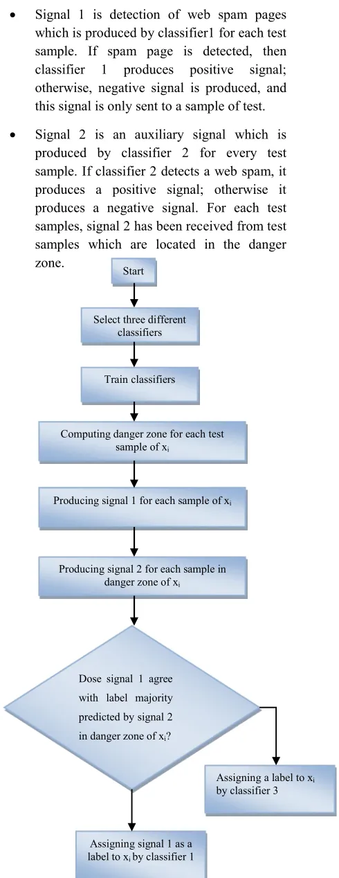
 Signal 1 is detection of web spam pages which is produced by classifier1 for each test sample. If spam page is detected, then classifier 1 produces positive signal; otherwise, negative signal is produced, and this signal is only sent to a sample of test.

 Signal 2 is an auxiliary signal which is produced by classifier 2 for every test sample. If classifier 2 detects a web spam, it produces a positive signal; otherwise it produces a negative signal. For each test samples, signal 2 has been received from test samples which are located in the danger zone.

Fig. 1. Process of the proposed method. Start

Select three different classifiers

Computing danger zone for each test sample of xi

Producing signal 1 for each sample of xi

Producing signal 2 for each sample in danger zone of xi

Dose signal 1 agree

with label majority

predicted by signal 2

in danger zone of xi?

Assigning signal 1 as a label to xi by classifier 1

Assigning a label to xi

(5)

Process of the proposed method has been shown in Figure 1, and its details are as follows:

Step1: Threevarious classifications are selected.

Step2: Classifiers are trained on dataset.

Step3: For each samplexi in test set, danger zone is calculated. In this way, at first, Euclidean distance of xi is calculated between xi test sample and other test samples. Then, average is calculated according to obtained distances. θ is the size of danger zone of xi and ||x_i - xj|| is Euclidean distance between xi test sample and other test samples . If the considered sample is shown with a feature vector; that is,

〈a1(x),a2(x),…an(x)〉, then Euclidean distance between two samples xi and xj is defined in formula (1).

||x_i - xj|| = ∑ (ar(xi) - ar xj ) 2 n

r=1 (1)

The average of Euclidean distances is defined in formula (2).

n θ = AVG

j=1

||x_i - xj||=

∑nj=1||x_i - xj||

n (2)

Step 4: for each sample xi, signal 1 is produced. This signal is sent to test sample xi. In other words, classifier 1 assigns a lable for each sample xi.

Step 5: for each test sample in danger zone of xi test sample (||x_i - xj||<=θ), signal 2 is produced and sent to test sample xi. In other words, classifier 2 assigns a label to the test sample available in danger zone of xi. This lable is used in final lable decision making for xi.

Step 6: Voting is performed in predicted lables obtained in stage 5. If majority lable of samples in danger zone of xi agree with xi lable predicted in stage 3, then the lable predicted by classifier 1 is assigned as final lable otherwise classifier 3 predicts the lable of xi test sample.

4 RESULTS EVALUATION

To evaluate performance of the proposed method, this section uses WEBSPAM-UK2007 data set in order to compare the proposed method with different classification methods.

4.1 Data set

In this part, data set of WEBSPAM-UK2007 has been used to compute evaluation criteria. This is a general accessible data set used in web

spam, and involves a huge set of spam /nonspam labeled by a group of volunteers collected from UK in May 2007. Dataset has been divided in two files: train set involving a small number of labeled hosts, and test set involving a large set of hosts without label. In this paper, we used train set for evaluation. This set involves 3849 hosts and features based on content and link. We have considered content analysis in our method, and it involves 96 features. Features employed in this paper are listed in Appendix I.

4.2 Evaluation criteria

In order to measure the classification performance of spam pages, we used the following criteria: precision, accuracy and FP rate.

Precision: it is the proportion of sample numbers that have been truly detected as positive (spam pages) to the total number of samples that have

been detected as

positive.

Precision= _{# Predicted Positive}True positive = _{True Positive}True positive₊_{False Positive} (3)

Accuracy: Accuracy refers to the proportion of samples that have been accurately classified to total number of samples.

Accuracy = True Positive+True Negative

True Positive + False Positive + True Negative + False Negative (4)

FP rate:

FP rate=_{False Positive+True Negative}False Positive

(5)

4.3 Comparing results

In this paper, we have used 10- fold cross-validation method. In order to evaluate the proposed method, the results of 5 combinations have been presented in table 1. In table 2, the obtained result from Vote, Staking and Grading have been presented by using the same combinations used in the proposed method. In table 3, the obtained result from base classification methods used in the proposed method have been shown. Tables 1-3 are listed in Appendix II.

(6)

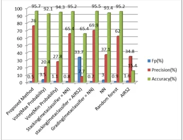
Fig. 2. Comparing the combination of NN, Random tree, C4.5 in the proposed method with other methods.

(7)

Fig. 4. Comparing the combination of Perceptron, C4.5, AIRS2 in the proposed method with other methods.

(8)

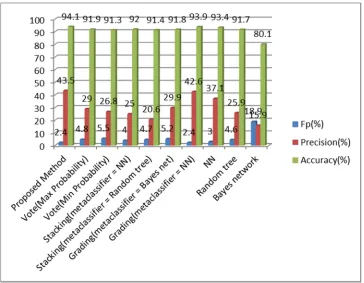
Fig. 6. Comparing the combination of Bayes network, Random tree, NN in the proposed method with other methods

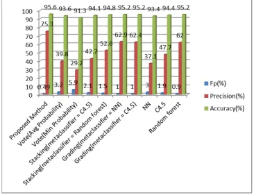
In experiments, the order of classifiers in combinations of the propose method have been consider in the form of classifier 1, classifier 2, classifier 3. In Figure 2, the combination of NN, Random tree, C4.5 in the proposed method is compared to other classification methods. As this figure shows, this combination with values of FP= 0.74%, precision=67.1% and accuracy= 95.3% has better results than other classification methods shown in figure 2. Figure 3 shows the comparison of the combination of NN, AIRS2, Random forest in the proposed method and other classifiers. This combination with the values of FP=0.5%, precision= 76% and accuracy=95.7% has better results in comparison to other classification methods shown in this figure. Figure 4 shows the comparison of the proposed method with the combination of Perceptron, C4.5, AIRS2 and other classifiers. This combination with the values of FP=0.4%, precision=68.3%, accuracy=95% has optimal results in comparison to other classification methods investigated in figure. As it can be observed in figure 5, the combination of NN, Random forest, C4.5 with the values of FP=0.49%, precision=75.3% and accuracy=95.6% has optimal results in comparison to other classification methods investigated in figure. Figure 6 shows the comparison results of the proposed method with the combination of Bayes net, Random tree, NN in comparison to other

classification methods. This combination with the values of FP=2.4%, precision=43.5% and accuracy=94.1% has better results than other classification methods investigated in the figure.

According to the results of tables 1-3, our method with the combination of NN, AIRS2, Random forest obtained the highest accuracy and precision among all methods with 95.7 and 76 success rates, respectively. It also can be observed that in the proposed method, the combination of Perceptron, C4.5, AIRS2 has best FP rate among all methods with 0.4% FP rate.

These results show that our proposed method is more effective in classification of spam pages.

5 CONCLUSION

In this paper, a combined method inspired from danger theory has been presented to detect web spam. The performance of the proposed method is evaluated using WEBSPAM-UK2007 data set. The results suggest a better performance for the proposed method in many cases when compared to the results obtained from base classifications methods and ensemble classifiers.

(9)

future, we will use a combination of danger theory and one of the algorithms of artificial immune system to detect web spam.

7 REFERENCES

[1] Najork M. Web Spam Detection. Encyclopedia of Database Systems. 2009;1:3520-3.

[2] Davison BD. Recognizing nepotistic links on the web. Artificial Intelligence for Web Search. 2000:23-8.

[3] Collins G. Latest search engine spam techniques. Aug 2004.

[4] Gyongyi Z, Garcia-Molina H. Web Spam Taxonomy. First International Workshop on Adversarial Information Retrieval on the Web (AIRWeb 2005). Chiba, Japan2005.

[5] Perkins A. The classification of search engine spam. 2001.

[6] Wu B, Goel V, Davison BD. Topical trustrank: Using topicality to combat web spam. Proceedings of the 15th international conference on World Wide Web: ACM; 2006. p. 63-72.

[7] Henzinger M, Motwani R, Silverstein C. Challenges in web search engines. SIGIR Forum. 2002;36:11-22.

[8] Abernethy J, Chapelle O, Castillo C. WITCH: A New Approach to Web Spam Detection. In Proceedings of the 4th International Workshop on Adversarial Information Retrieval on the Web (AIRWeb}2008.

[9] Matzinger P. The real function of the immune system or tolerance and the four d's (danger, death, destruction and distress). American Society for Microbiology. 1996.

[10]Matzinger P. The danger model: a renewed sense of self. Science. 2002;296:301-5.

[11]Ntoulas A, Najork M, Manasse M, Fetterly M. Detecting spam web pages through content analysis. the 15th International World Wide Web Conference. Edinburgh, ScotlandMay 2006. p. 83–92.

[12]Amitay E, Carmel D, Darlow A, Lempel R, Soffer A. The connectivity sonar: Detecting site functionality by structural patterns. the 14th ACM Conference on Hypertext and Hypermedia. Nottingham, UKAug 2003. p. 38–47.

[13]Prieto V, Álvarez M, López-García R, Cacheda F. Analysis and Detection of Web Spam by Means of Web Content. In: Salampasis M, Larsen B, editors. Multidisciplinary Information Retrieval: Springer Berlin Heidelberg; 2012. p. 43-57.

[14]Karimpour J, Noroozi A, Alizadeh S. Web Spam Detection by Learning from Small Labeled Samples. International Journal of Computer Applications. 2012;50:1-5.

[15]Rungsawang A, Taweesiriwate A, Manaskasemsak B. Spam Host Detection Using Ant Colony Optimization. In: Park JJ, Arabnia H, Chang H-B, Shon T, editors. IT Convergence and Services: Springer Netherlands; 2011. p. 13-21.

[16]Silva RM, Yamakami A, Alimeida TA. An Analysis of Machine Learning Methods for Spam Host Detection. 11th International Conference on Machine Learning and Applications (ICMLA)2012.

[17]Becchetti L, Castillo C, Donato D, Leonardi S, Baeza-Yates RA. Link-Based Characterization and Detection of Web Spam. AIRWeb 2006. Seattle, Washington, USA2006. p. 1-8.

[18]Castillo C, Donato D, Gionis A, Murdock V, Silvestri F. Know your neighbors: web spam detection using the web topology. Proceedings of the 30th annual international ACM SIGIR conference on Research and development in information retrieval. Amsterdam, The Netherlands: ACM; 2007. p. 423-30.

[19]Dai N, Davison BD, Qi X. Looking into the past to better classify web spam. Proceedings of the 5th International Workshop on Adversarial Information Retrieval on the Web. Madrid, Spain: ACM; 2009. p. 1-8.

[20]Anderson CC, Matzinger P. Danger: the view from the bottom of the cliff. Seminars in immunology: Academic Press; 2000. p. 231-8. [21]Gallucci S, Matzinger P. Danger signals: SOS

to the immune system. Current opinion in immunology. 2001;13:114-9.

[22]Bretscher P, Cohn M. A Theory of Self-Nonself Discrimination Paralysis and induction involve the recognition of one and two determinants on an antigen, respectively. Science. 1970;169:1042-9.

[23]Aickelin U, Cayzer S. The danger theory and its application to artificial immune systems. arXiv preprint arXiv:08013549. 2008.

[24]Aickelin U, Bentley P, Cayzer S, Kim J, McLeod J. Danger theory: The link between AIS and IDS? Artificial Immune Systems: Springer; 2003. p. 147-55.

[25]Aickelin U, Greensmith J. Sensing danger: Innate immunology for intrusion detection. Information Security Technical Report. 2007;12:218-27.

(10)

Interesting Information: University of Kent; 2006.

[27]Zhu Y, Tan Y. A Danger Theory Inspired Learning Model and Its Application to Spam Detection. In: Tan Y, Shi Y, Chai Y, Wang G, editors. Advances in Swarm Intelligence: Springer Berlin Heidelberg; 2011. p. 382-9. [28]Quinlan JR. C4. 5: programs for machine

learning: Morgan kaufmann; 1993.

[29]Friedman N, Geiger D, Goldszmidt M. Bayesian network classifiers. Machine learning. 1997;29:131-63.

(11)

Appendix I

List of content features in WEBSPAMUK2007 Dataset.

HST_1

Number of words in the page (home page = hp) HST_2

Number of words in the title (hp) HST_3

Average word length (hp) HST_4

Fraction of anchor text (hp) HST_5

Fraction of visible text (hp) HST_6

Compression rate of the hp HST_7

Top 100 corpus precision (hp) HST_8

Top 100 corpus recall (hp) HST_12

Top 100 queries precision (hp) HST_16

Top 100 queries recall (hp) HST_20

Entropy (hp) HST_24

Independent LH (hp) HMG_25

Number of words in the page (page with max PageRank in the host = mp)

HMG_26

Number of words in the title (mp) HMG_27

Average word length (mp) HMG_28

Fraction of anchor text (mp)

HMG_29

Fraction of visible text (mp) HMG_30

Compression rate (mp) HMG_31

Top 100 corpus precision (mp) HMG_32

Top 100 corpus recall (mp) HMG_36

Top 100 queries precision (mp) HMG_40

Top 100 queries recall (mp) HMG_44

Entropy (mp) HMG_48

Independent LH (mp) AVG_49

Number of words in the page (average value for all pages in the host)

AVG_50

Number of words in the title (average value for all pages in the host)

AVG_51

Average word length (average value for all pages in the host)

AVG_52

Fraction of anchor text (average value for all pages in the host)

AVG_53

Fraction of visible text (average value for all pages in the host)

AVG_54

(12)

Top 100 corpus precision (average value for all pages in the host)

AVG_56

AVG_57

AVG_58

AVG_59

Top 100 corpus recall (average value for all pages in the host)

AVG_60

AVG_61

AVG_62

AVG_63

Top 100 queries precision (average value for all pages in the host)

AVG_64

AVG_65

AVG_66

AVG_67

Top 100 queries recall (average value for all pages in the host)

AVG_68

AVG_69

AVG_70

AVG_71

Entropy (average value for all pages in the host) AVG_72

Independent LH (average value for all pages in the host) STD_73

Number of words in the page (Standard deviation for all pages in the host)

STD_74

Number of words in the title (Standard deviation for all pages in the host)

STD_75

Average word length (Standard deviation for all pages in the host)

STD_76

Fraction of anchor text (Standard deviation for all pages in the host)

STD_77

Fraction of visible text (Standard deviation for all pages in the host)

STD_78

Compression rate in the home page (Standard deviation for all pages in the host)

STD_79

Top 100 corpus precision (Standard deviation for all pages in the host)

STD_80

STD_81

STD_82

STD_83

Top 100 corpus recall (Standard deviation for all pages in the host)

STD_84

STD_85

STD_86

STD_87

Top 100 queries precision (Standard deviation for all pages in the host)

STD_88

STD_89

STD_90

STD_91

Top 100 queries recall (Standard deviation for all pages in the host)

STD_92

STD_93

STD_94

STD_95

Entropy (Standard deviation for all pages in the host) STD_96

(13)

Appendix II

Tables

Table1: The obtained results from the proposed method.

Accuracy (%) Precision (%) FP rate (%) Combination

(Classifier 1, classifier 2, classifier 3 )

95.3 67.1

0.74 NN, Random tree, c4.5

95.7 76

0.5 NN, AIRS2,Random forest

95 68.3 0.4 Perceptron,C4.5, AIRS2 95.6 75.3 0.49 NN, Random forest, c4.5

94.1 43.5

2.4 Bayes net, Random tree, NN

Table2: The obtained results from ensemble classifiers.

Accuracy (%) Precision (%) FP rate (%) Method Combination 91.3 29.2 5.9 Vote(Combination Rule= Max Probability)

NN, Random tree, c4.5

93.1 32

3.9 Vote(Combination Rule=Min Probability)

93.9 39.2

2 Stacking(meta-classifier = NN)

93.9 39.4

2.1 stacking(meta-classifier = Random tree)

95.1 58.4

1.2 Grading(meta-classifier = NN)

94.8 52.8

1.6 Grading(meta-classifier = C4.5)

92.1 20.4

3.5 Vote(Combination Rule=Max Probability)

NN, AIRS2,Random forest

94.3 27.8

1.1 Vote(Combination Rule=Avg Probability)

95.2 65.4

0.8 Stacking(meta-classifier = NN)

65.4 7.7

33.7 stacking(meta-classifier = AIRS2)

95.5 69.9

88.9 19.9

Perceptron,C4.5, AIRS2

94.7 58.6

94.8 40

0.1 Stacking(meta-classifier =Perceptron )

91 16.1

4.7 Stacking(meta-classifier = AIRS2 )

93.3 16.9

1.8 Grading(meta-classifier = Perceptron)

94.5 47

1 Grading(meta-classifier = c4.5)

93.6 39.8

NN, Random forest, c4.5

91.3 29.2

94.1 42.7

2.1 Stacking(meta-classifier = c4.5)

94.8 52.6

1.5 Stacking(meta-classifier = Random forest)

95.2 62.9

1 Grading(meta-classifier = NN)

95.2 62.4

1 Grading(meta-classifier = c4.5)

91.9 29

Bayes net, Random tree, NN

91.3 26.8

92 25

4 Stacking(meta-classifier = NN)

91.4 20.6

4.7 Stacking(meta-classifier = Random tree)

91.8 29.9

5.2 Grading(meta-classifier = Bayes net)

93.9 42.6

Table3: The obtained results from base classifiers.