International Journal of New Innovations in Engineering and Technology
Volume 4 Issue 2 – January 2016 16 ISSN : 2319-6319
Comparison of Two Way Join Algorithms
used in MapReduce Frame work for handling
BigData
Suren kumar Sahu
Department of Computer Science and Engineering Gandhi Engineering College,Bhubaneswar
Lambodar Jena
Department of Computer Science and Engineering Gandhi Engineering College,Bhubaneswar
Santosh Satapthy
Department of Computer Science and Engineering Gandhi Engineering College,Bhubaneswar
S.Gayatri Dora
Department of Computer Science and Engineering Regional Institute of Education,Bhubaneswar
Abstract-Due to the advent of new technologies, devices, and communication means like social networking sites, the amount of data produced by mankind is growing rapidly every year. The amount of data produced by us from the beginning of time till 2003 was 5 billion gigabytes. A vast amount of research going on into how best to handle and process huge amounts of data which is generated by different media and social networks. One such idea for processing enormous quantities of data is Google’s Map/Reduce. MapReduce is the heart of Hadoop. It is this programming paradigm that allows for massive scalability across hundreds or thousands of servers in a Hadoop cluster. The MapReduce concept is fairly simple to understand for those who are familiar with clustered scale-out data processing solutions. The MapReduce framework is increasingly being used widely to analyze large volumes of data. One of the techniques that framework is join algorithm. Join algorithms can be divided into two groups: Reduce-side join and Map-side join. The aim of our work is to compare existing join algorithms which are used by the MapReduce framework. We have compared Reducer-side merge join and Map-side replication-join in terms of pre-processing, the number of phases involved, whether it is sensitive to data skew, whether there is need for distributed Cache, memory overflow.
Key Words:
Join algorithms, MapReduce, optimization.Semi join,Bloom Filter,Hadoop
I. INTRODUCTION
Map/Reduce[1] was first introduced by Google engineers - Jeffrey Dean and Sanjay Ghemawat [9]. It was designed for and is still used at Google for processing large amounts of raw data (like crawled documents and web-request logs) to produce various kinds of derived data (like inverted indices, web-page summaries, etc.). It isa simple yet powerful framework for implementing distributed applications without having extensive prior knowledge of the intricacies involved in a distributed system. It is highly scalable and works on a cluster of commodity machines with integrated mechanisms for fault tolerance.Data-intensive applications include large-scale data warehouse systems, cloud computing, data-intensive analysis. These applications have their own specific computational workload. For example, analytic systems produce relatively rare updates but heavy select operation with millions of records to be processed, often with aggregations.
International Journal of New Innovations in Engineering and Technology
Volume 4 Issue 2 – January 2016 17 ISSN : 2319-6319 O and CPU costs. Join algorithms is not directly supported in MapReduce. There are some approaches to solve this problem by using a high-level language PigLatin, HiveQL for SQL queries or implementing algorithms from research papers. The aim of this work is to generalize and compare existing equi-join algorithms with some optimization techniques.
II.JOIN ALGORITHMS AND OPTIMIZATION TECHNIQUES
In this section we consider various techniques of two-way joins in MapReduce framework. Join algorithms can be divided into two groups: Reduce-side join and Map-side join. The pseudo code presented in Listings, where R – right dataset, L –left dataset, V – line from file, Key – join key, that was parsed from a tuple, in this context tuple is V.
2.1 Two-Way Joins
2.1.1 Reduce-Side join
Reduce-side join is an algorithm which performs data pre-processing in Map phase, and direct join is done during the Reduce phase. Join of this type is the most general without any restriction on the data. Reduce-side join is the most time-consuming, because it contains an additional phase and transmits data over the network from one phase to another. In addition, the algorithm has to pass information about source of data through the network. The main objective of the improvement is to reduce the data transmission over the network from the Map task to the Reduce task by filtering the original data through semi-joins. Another disadvantage of this class of algorithms is the sensitivity to the data skew, which can be addressed by replacing the default hash partitioner with a range partitioner.
There are three algorithms in this group:
General reducer-side join Optimized reducer-side join Hybrid Hadoop join
General reducer-side join is the simplest one. The same algorithms are called Standard Repartition Join in [6]. The abbreviation is GRSJ and pseudo code is presented below:
General reducer-side join:
---
Map (K: null, V from R or L)Tag = bit from name of R or L;
emit (Key, pair(V,Tag));
Reduce (K’: join key, LV: list of V with key K’)
create buffers B r and B l for R and L; for t in LV do
add t.v to B r or B l by t.Tag; for r in B r do
for l in B l do
International Journal of New Innovations in Engineering and Technology
Volume 4 Issue 2 – January 2016 18 ISSN : 2319-6319 Figure-1. Reduce Side Join - Two Way
This algorithm has both Map and Reduce phases. In the Map phase, data are read from two sources and tags are attached to the value to identify the source of a key/value pair. As the key is not effecting by this tagging, so we can use the standard hash partitioner. In Reduce phase, data with the same key and different tags are joined with nested-loop algorithm. The problems of this approach are that the reducer should have sufficient memory for all records with a same key; and the algorithm sensitivity to the data skew.
2.1.2 Map-Side join
Map-side join is an algorithm without Reduce phase. This kind of join can be divided into two groups. First of them is partition join, when data previously partitioned into the same number of parts with the same partitioner. The relevant parts will be joined during the Map phase. This map-side join is sensitive to the data skew. The second is in memory join, when the smaller dataset send whole to all mappers and bigger dataset is partitioned over the mappers. The problem with this type of join occurs when the smaller of the sets cannot fit in memory.
There are three methods to avoid this problem: JDBM-based map join,
Multi-phase map join, Reversed map join
Limitation of Map-Side Join:
Limitation Why
All datasets must be sorted using the same comparator The sort ordering of the data in each dataset must be identical for datasets to be joined.
All datasets must be partitioned using the same partitioner.
A given key has to be in the same partition in each dataset so that all partitions that can hold a key are joined together.
The number of partitions in datasets must be identical A given key has to be in the same partition in each he dataset so that all partitions that can hold a key are joined together.
2.1.3 Broadcast Join
International Journal of New Innovations in Engineering and Technology
Volume 4 Issue 2 – January 2016 19 ISSN : 2319-6319 instance, a small users database may need to be joined with a large log. This small dataset can be simply replicated on all the machines. This can be achieved by simply using -files or -archive directive to send the file to each machine while invoking the Hadoop job. Broadcast join is a Map-only algorithm.
Map Phase
The Mapper loads the small dataset into memory and calls the map function for each tuple from the bigger dataset. For each (key, value), the map function probes the in- memory dataset and finds matches. This process can be further optimized by loading the small dataset into a Hashtable. It then writes out the joined tuples. The below shown configure function is part of the Mapper class and is called once for every Mapper. The below code reads the ‘broadcasted’ file and loads the same into an in- memory hash table.
Loading the small dataset into a Hash table:
---
public void configure ( JobConf conf ) {//Read the broadcasted file
T1 = new File ( conf . get (" broadcast . file ")); //Hashtable to store the tuples
ht = new HashMap < String , ArrayList < String > >() ; BufferedReader br = null;
String line = null; try{
br = new BufferedReader (new FileReader ( T1 )); while(( line = br . readLine () ) !=null)
{
String record [] = line . split ("\t" , 2) ; if( record . length == 2)
{
//Insert into Hashtable if( ht . containsKey ( record [0]) ) {
ht . get ( record [0]) . add ( record [1]) ; }
else {
ArrayList < String > value = new ArrayList < String >() ;
value . add ( record [1]) ; ht . put ( record [0] , value ); }
} } }
catch( Exception e) {
e. printStackTrace () ; }
}
---
The next piece of code is the actual map function that receives the records from the HDFS and probes the HashTable containing the tuples from the broadcasted file. Notice that it takes care of duplicate keys as well.
Broadcast Join Map Function:
---
public void map( LongWritable lineNumber , Text value ,OutputCollector < Text , Text > output , Reporter reporter )
throws IOException {
String [] rightRecord = value . toString () . split ("\t" ,2); if( rightRecord . length == 2)
{
International Journal of New Innovations in Engineering and Technology
Volume 4 Issue 2 – January 2016 20 ISSN : 2319-6319 {
output . collect (new Text ( rightRecord [0]) , new Text ( leftRecord + "\t" + rightRecord [1]) );
} } }
---
Broadcast Join benefits from the fact that it uses a small ‘local’ storage on the individual nodes instead of the HDFS. This makes it possible to load the entire dataset into an in-memory hash table, access to which is very fast. But on the down side, it will run into problems when both the datasets are large and neither of them can be stored locally on the individual nodes.
III.SEMIJOIN
Sometimes a large portion of the data set does not take part in the join. Deleting of tuples that will not be used in join significantly reduces the amount of data transferred over the network and the size of the dataset for the join. This preprocessing can be carried out using semi-joins by selection or by a bitwise filter.
However, these filtering techniques introduce some cost (an additional MR job), so the semi-join can improve the performance of the system only if the join key has low selectivity. There are three ways to implement the semi-join operation:
a semi-join using bloom-filter, semi-join using selection, an adaptive semi-join.
Bloom-filter is a bit array that defines a membership of element in the set. False positive answers are possible, but there are no false-negative responses in the solution of the containment problem. The accuracy of the containment problem solution depends on the size of the bitmap and on the number of elements in the set. These parameters are set by the user. It is known that for a bitmap of fixed size m and for the data set of n tuples, the optimal number of hash functions is k=0.6931*m/n. In the context of MapReduce, the semi-join is performed in two jobs. The first job consists of the Map phase, in which keys from one set are selected and added to the Bloom-filter. The Reduce phase combines several Bloom-filters from first phase into one. The second job consists only of the Map phase, which filters the second data set with a Bloom-filter constructed in previous job.
The accuracy of this approach can be improved by increasing the size of the bitmap. However in this case, a larger bitmap consumes more amounts of memory. The advantage of this method is its the compactness. The performance of the semi-join using Bloom-filter highly depends on the balance between the Bloom-filter size, which increases the time needed for its reconstruction of the filter in the second job, and the number of false positive responses in the containment solution. The large size of the data set can seriously degrade the performance of the join.
Semi-join using Bloom Filter
---
Job 1: construct Bloom filter
Map (K:null, V from L) Add Key to BloomFilter Bl
close() //for Map phase
emit(null, Bl);
Reduce (K’: key, LV) //only 1 Reducer
for l in LV do
union filters by operation Or
close() // for Reduce phase
write resulting filter into file;
Job 2: filter dataset
init() //for Map phase
read filter from file in Bl Map (K:null, V from R) if (Key in Bl) then
International Journal of New Innovations in Engineering and Technology
Volume 4 Issue 2 – January 2016 21 ISSN : 2319-6319
Job 3: do join with L dataset and filtered dataset from Job 2.
---
Semi join with selection:
--- Job 1: find unique keys
Map (K:null, V from L) Create HashMap H; if (not Key in H) then
add Key to H; emit (Key, null);
Reduce (K’: key, LV) //only one Reducer emit (null,key);
Job 2: filter dataset
init() //for Map phase
add to HashMap H unique keys from job 1; Map (K:null, V from R)
if (Key in H) then emit (null,V);
Job 3: do join with L dataset and filtered dataset from Job 2.
---
Semi-join with selection extracts unique keys and constructs a hash table. The second set is filtered by the hash table constructed in the previous step. In the context of MapReduce, the semi-join is performed in two jobs. Unique keys are selected during the Map phase of the first job and then they are combined into one file during the Map phase. The second job consists of only the Map phase, which filters out the second set. The semi-join using selection has some limitations. Hash table in memory, based on records of unique keys, can be very large, and depends on the key size and the number of different keys.
The Adaptive semijoin is performed in one job, but filters the original data on the flight during the join. Similar to the Reduce-side join at the Map phase the keys from two data sets are read and values are set equal to tags which identify the source of the keys. At the Reduce phase keys with different tags are selected. The disadvantage of this approach is that additional information about the source of data is transmitted over the network.
Adaptive Semijoin
---
Job 1: find keys which are present in two datasetsMap (K:null, V from R or L) Tag = bit from name of R or L; emit (Key,Tag);
Reduce (K’: join key, LV: list of V with key K’) Val = first value from LV; for t in LV do
if (not Val==Val2) then emit (null, K’);
Job 2: before joining it is necessary to filter the smaller dataset
dataset by keys from the Job 1 that willbe loaded into hash map. Then the bigger dataset is joined with filtered one
---
VI.EXPERIMENTS AND ANALYSIS
Dataset
Data are the set of tuples, which attributes are separated by a comma. Tuple is split into a pair of a key and a value, where value is the remaining attributes. Generation of synthetic data was done as in [4]. Join keys are distributed randomly except experiment with the data skew.
Cluster configuration
International Journal of New Innovations in Engineering and Technology
Volume 4 Issue 2 – January 2016 22 ISSN : 2319-6319 MSPJ 2 data 1 - yes - Part size is large Hash
Cluster consists of three virtual machines, where one of them is master and slave at the same time, the remaining two are the slaves. Host configuration consists of 1 processor, 512 mb of memory for nodes, 5 gb is the disk size. Hadoop 20.203.0 runs on Ubuntu 10.10.
The General Case:
The base idea of this experiment is to compare executions time of different phases of various algorithms. Some parameters are fixed: the number of Map and Reduce tasks is 3, the input size is 10^ 4 x10^ 5 and 10^ 6 x10^ 6 tuples.
Performance of two-way joins on increasing input data size
A series of experiments were conducted to compare the runtime and scalability of the various algorithms. The first of these involved running the three two-way algorithms mentioned earlier on increasing data sizes .
Both datasets involved in the joins had the following characteristics -
• Same number of tuples • Same key space • #keys = 1/10 #tuples
We tested on two kinds of key distributions as shown in Figure 2 and Figure 3. In the case of skewed data, one of the datasets had a key that was repeated 50% of the times. Which means that given n rows, n / 2 of them were the same key. The other dataset had uniform key distribution
Concentrating first on the Uniform Key Distribution graph (Figure 2), it can be seen that all the three algorithms gave comparable numbers at lower input data sizes. But Map-side join always performed the best, even with large input datasets. Broadcast join deteriorated the fastest as the data size increased. This is because a larger file had to be replicated across all the machines in the cluster as the input size increased. Figure 3 shows something interesting. Map-side join gave a worse time than the other two algorithms for the input with 5 million rows when then input dataset had skewed key distribution. This can be attributed to the unequal partitioning that will occur due to the skew.
Apart from testing for runtimes, we also checked for the amount of data transferred over the network from the machines running the Reduce tasks. A simple number like the number of bytes transferred might not be very meaningful. Hence we took the ratio as
International Journal of New Innovations in Engineering and Technology
Volume 4 Issue 2 – January 2016 23 ISSN : 2319-6319 Figure-2. Uniform Key Distribution
International Journal of New Innovations in Engineering and Technology
Volume 4 Issue 2 – January 2016 24 ISSN : 2319-6319 Table -1 Uniform Key Distribution
Table -2 Skewed Data Distribution
There are two main things worth noticing in Table 1 and Table 2. The first is that the Data Shuffle ratio remains around 1.14 for both uniform and skewed key distribution. This is because as the data size increases, Hadoop is able to better manage data distribution and data locality. The other thing is that though Map-Side performed best most of the times, it took an average time of 50.29 seconds (uniform key distribution).and 49.57 seconds (skewed key distribution) for the pre-partitioning phase. This may not seem a lot, but is likely to be quite high if the input datasets are much larger than the ones used in this experiment.
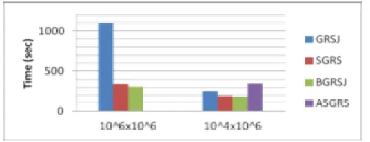
Semi-Join Comparisions:
The main idea of this experiment is to compare different semi-join algorithms. These parameters are fixed: the number of Map and Reduce tasks is 3, the bitmap size of Bloom-filter is 25*10 5 , the number of hash-functions in Bloom-filter is 173, built-in Jenkins hash algorithm is used in Bloom-filter. Adaptive semi-join (ASGRSJ) does not finish because of memory overflow. The abbreviation of Bloom-filter semi-join for GRSJ is BGRSJ. The abbreviation of semi-join with selection for GRSJ is SGRSJ respectively.
International Journal of New Innovations in Engineering and Technology
Volume 4 Issue 2 – January 2016 25 ISSN : 2319-6319 V.CONCLUSION
We explored the practicality of using Map/Reduce for joining datasets and found it quite easy to use and implement over different sizes of cluster. In this work we found some quite interesting results from our experiments on Join algorithms using Map/Reduce. Even though our clusters were of relatively small sizes, we could notice from our experiments how the Hadoop framework exploited the cluster architecture when more nodes were added (as was seen with the Data Shuffle ratio that remained the same throughout our experiments). This gave us a first-hand feel of why Hadoop seems to be enjoying such a high popularity among data warehousing specialists. We found that Map-Side joins performs the best when the datasets have relatively uniform key distribution. But this comes at the cost of a pre-processing step. Broadcast Join is a better option when one of the datasets is much smaller compared to the other and the dataset is small enough to be easily replicated across all the machines in the cluster. It deteriorated the fastest when the input data size was increased. Reduce-Side Join gave almost the same performance for both uniform and skewed key distributions whereas Map-Side Join seemed to give slightly unpredictable results with skewed data.
In this work we describe the state of the art in the area of massive parallel processing, presented our comparative study of these algorithms reduced side join,map side join ,broad cast join and semi-join.In future work multi way join can be tested and analysed using more number of Hadoop clusters.
REFERENCES
[1] Apache cassandra.
[2] Apache hadoop. Website. http://hadoop.apache.org. [3] Cloudera inc. http://www.cloudera.com.
[4] Hadoop wiki - poweredby. http://wiki.apache.org/hadoop/PoweredBy.
[5] A. Abouzeid, K. Bajda-Pawlikowski, D. Abadi, A. Silberschatz, and A. Rasin. Hadoopdb: an architectural hybrid of mapreduce and dbms Technologies for ana lytical workloads. Proc. VLDB Endow., 2(1):922–933, 2009.
[6] S. Blanas, J. M. Patel, V. Ercegovac, J. Rao, E. J. Shekita, and Y. Tian. A comparison of join algorithms for log processing in mapreduce. In SIGMOD ’10:Proceedings of the 2010 international conference on Management of data, pages 975–986, New York, NY, USA, 2010. ACM.
[7] R. Chaiken, B. Jenkins, P.-A. Larson, B. Ramsey, D. Shakib, S. Weaver, and J. Zhou. Scope: easy and efficient parallel processing of massive data sets. Proc.VLDB Endow., 1(2):1265–1276, 2008.
[8] F. Chang, J. Dean, S. Ghemawat, W. C. Hsieh, D. A. Wallach, M. Burrows, T. Chandra, A. Fikes, and R. E. Gruber. Bigtable: a distributed storage system for structured data. In OSDI ’06: Proceedings of the 7th USENIX Symposium on Operating Systems Design and Implementation, pages 15–15, Berkeley, CA,USA, 2006. USENIX Association.