Image Mining for Mammogram Classification to detect breast cancer by Association Reverse Rule Using Statistical and GLCM features

(1)

Volume 5 Issue 2– June 2016

20

ISSN : 2319-6319

Architecture for Canonic RFFT based on

Canonic Sign Digit Multiplier and Carry Select

Adder

Pradnya Zode

Research Scholar, Department of Electronics Engineering. G.H. Raisoni College of engineering, Nagpur, Maharashtra, India

Dr.A.Y.Deshmukh

Professor, Department of Electronics Engineering. G.H. Raisoni College of engineering, Nagpur, Maharashtra, India

Abstract-This paper presents architectures for computing Fast Fourier transform (FFT) in Decimation-In-Time (DIT) algorithm using a new approach called as canonic FFT for real valued signals. N output complex signals are computed by an N-point FFT using N complex signals in DIT or decimation-in-frequency (DIF) algorithm. The FFT involves stages of calculations where every stage calculates N complex signal; N is assumed to be power of two. Each phase of the FFT have to calculate only N signal values, as input data consist of only N samples which may be real or imaginary value. Any more than N samples computed at any FFT stage are naturally repetitive. The canonic FFT is the FFT where the calculations at each stage of the FFT on the input data signal should be equal. In the proposed N-point FFT structure, N calculations are done on the input data at each stage of the FFT. Canonic RFFT structures based on decimation-in-time and decimation-in-frequency were presented earlier. This paper presents an approach to calculate canonic RFFT by implementing canonical signed digit (CSD) multiplier and carry select adder (CSLA) adder. The Canonic Sign Digit (CSD) a type of number representation as well as an algorithm for multiplying one number by another.The multiplication done on the CSD numbers is fast. CSLA is a fast adder in all adders which is used for perform fast arithmetic operations.

Keywords- Canonic FFT, Real-Valued FFT, Decimation-in-time, Canonic sign digit (CSD) multiplier, Carry select adder (CSLA)

I.INTRODUCTION

(2)

21

ISSN : 2319-6319 Canonic real-valued FFT structures using decimation-in-time (DIT) and decimation-in-frequency (DIF) approach is presented very well in reference [11].To design all-purpose RFFT architecture which is canonic regarding to the number of signals at the output of each intermediate stage of FFT using CSD multiplier and CSL adder is the main aim of this article. It means for an N-point RFFT the total number of values calculated at the output of each intermediate stage should be N. Moreover, every stage must contain utmost N/2 real butteries rather than N/2 complex butteries. In this paper, it is shown that it is conceivable to form just N free values at every stage for a N-point RFFT. The canonical signed digit (CSD) representation is one of the signed digit (SD) representations with exclusive features which make it useful in various DSP applications focusing on low- power, efficient-area and high-speed arithmetic.The use of CSD number system both to represent fixed-point numbers and to describe an efficient shift and-add algorithm for multiplying a number by a fixed coefficient is well known [7].The exclusive features of CSD representation are that it does not allow two successive digits to be non-zero and the representation must have the fewest number of non-zero digits. Carry Select adder is the fastest adder among the Conventional adder. The adder used in this paper is an area efficient Carry select adder by sharing the common Boolean logic term [9].

This paper is organized as follows. Introduction to Canonical Signed Digit Multiplier is given in Section II. Section III addresses the Carry Select Adder. Section IV presents the working of Real Fast Fourier Transform. Section V describes the different Canonic Decimation in time RFFT architectures. Section VI presents the implementations of all canonic RFFT architectures and their results with respect to power and area. Finally some conclusions are given in Section VII.

II.CANONICALSIGNEDDIGITMULTIPLIER

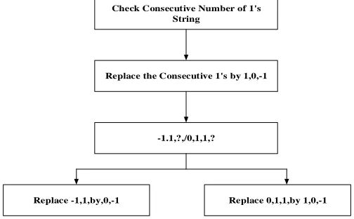
In any classic multiplier, multiplication is done by shifts producing partial products and after that adding all the partial products. Therefore multiplication of two "N" bits will create NxN partial products and thus (N-1) adders will require if two-input "N" bit adders are used. So the number of hardware component increases also the time required for multiplication. Thus there is need of multiplier which creates less partial product with high speed. Fast multiplication can be achieved by using canonical signed digit (CSD) to speed-up computations.CSD is a type of number representation [8]. CSD representation of numbers can reduce the complexity of the hardware required to realize a FFT. The CSD number system is a signed digit number system that minimizes the number of non-zero bits and so can reduce the number of partial product additions in a multiplier [7]. The CSD number representation is based on ternary bit set where each bit can take value either -1, 0, or +l. Adjacent CSD bits are never both non-zero.CSD multiplier suits best to our requirement. Proposed CSD multiplier is extremely proficient method for multiplication; it decreases the number of partial products by utilizing redundancy of sign code CSD multiplier. As number of partial products are reduced, it is more equipment productive, so it require less time for multiplication and low power utilization than typical multiplier. For CSD multiplier first the number which is to be multiplied has to convert to CSD representation. The procedure of conversion is shown in the flowchart of figure.1.

Check Consecutive Number of 1's String

Replace the Consecutive 1's by 1,0,-1

-1.1,?,/0,1,1,?

Replace -1,1,by,0,-1 Replace 0,1,1,by 1,0,-1

(3)

22

ISSN : 2319-6319 After conversion the multiplication is performed as follows

• Convert the Multiplicand into CSDC

• Generate N X N bits partial products

• Add the partial products

• Convert addition results into 2’s complement format.

III.CARRY SELECT ADDER

Carry Select adder is known to be the fastest adder among the Conventional adder. The adder used in this paper is an area efficient Carry select adder by sharing the common Boolean logic term. It consists of two ripple adder and one multiplex. In this adder structure one XOR gate and one inverter gate are needed for summation operation as well as one AND and one OR gate are needed for carry out operation. It takes two inputs A and B and creates partial sum of them [9]. Then this is given as an input to the multiplex which chooses the correct output based on actual carry. Least measure of power utilization and little carry output delay is a fundamental reason behind building up a propose CSLA.

All the architectures designed in this paper are designed using above mentioned Canonical Signed Digit Multiplier and Carry Select Adder.

IV. REAL FAST FOURIER TRANSFORM

The wide usage of DFT’s in variety of Digital Signal Processing applications is the motivation to design efficient architectures for the implementation of FFT’s. DFT is the representation of a sequence {x (n)} by samples of its frequency spectrum X (ω). As a result, computation of the N-point DFT corresponds to the computation of N input samples of the Fourier transform at N equally spaced frequencies ω = 2πk/N. Considering input signal x[n] to be complex, N complex multiplications and (N-1) complex additions are required to compute each value of the DFT, if computed directly. The N-point Discrete Fourier Transform (DFT) for an input signals x(n) is given as [10]:

kn N N

n N kn j

W

n

x

e





 





1

0 / 2 1

N

0 n

)

(

x(n)

X(k)



Where k=0,1,2……,N-1 and In 1965,Cooley and Tukey has proposed an algorithm for computing DFT of a signal which is known as FFT.FFT is a fast algorithm [10] which takes Nlog2N arithmetic operations to compute DFT. The input sequence x[n] is

considered to be real valued sequence for the RFFT. For real input values of x[n], it can be shown that [10]

Im(x[n]) = 0

X[k] =

In this case, there are conjugate output pairs, i.e., X[k] and X[N-k], for k = 1,2,…. In this way, just outputs should be calculated in a N-point RFFT flow-diagram, as either X[k] or X[N-k] can be calculated, along with two real yield signals X[0] and X[N/2] .The total number of purely real and purely imaginary signal values is N.

Any N-point RFFT, where N is power of-two, can be acquired by combination two N/2 – point RFFTs utilizing the DIT property calculation. This property can be expressed as

=

(4)

23

ISSN : 2319-6319

Where represent one even part RFFT and represent another

RFFTs for the odd part of the inputs. Twiddle variables should be multiplied to the odd part before the butterflies at the last stage.

V. CANONIC DECIMATION-IN-TIME RFFT

In this part of the paper, the flow graphs for canonic DIT RFFT calculations are presented which are ensured to have N signals at every stage. For all flow graphs it is assumed that the node shown by sign o is a real signal and shown by sign □ shows an imaginary signal [11]. Solid lines are used to represent real data paths and dashed lines are used to show imaginary data paths [11].

5.1 4-point canonic RFFT [11]

A 4-point canonic DIT RFFT flow-graph is shown in Figure 1. In the 4-point RFFT, as X [1] and X [3] are complex conjugates of each other, X [3] can be eliminated by removing the bottom butterfly at the second stage. The calculations of real and imaginary parts of X [1] are separated as shown in figure 2. The number of inputs, outputs and signal values at the in-between stages are all the same and equal 4 which is the size of FFT.

x(2)

x(1)

x(3)

-j

-1 -1

-1

X(1r)

X(2)

X(1i)

x(0) X(0)

Figure 2. Flow-graph of a canonic 4-point DIT RFFT [11]

(5)

24

ISSN : 2319-6319

X(0)

X(4)

X(2)

X(6)

X(1)

X(5)

X(3)

-1

X(7) -j -1

-j -1

X(0) X(1r) X(2r) X(1i) X(4) -1

-1

X(5r) X(2i) X(5i) -j -1 W1

(6)

25

ISSN : 2319-6319 X(0) X(8) X(4) X(12) X(2) X(10) X(6) X(14) X(1) X(9) X(5) X(13) X(11) X(7) X(15) -1 -1 -1 -1 -1 -1 -1 -1 -1 -1 -1 -1 -j -j -j -j -1 -1 -1 -1 X(1r) X(2r) X(1i) X(4r) X(5r) X(2i) X(5i) X(8) X(9r) X(10r) X(9i) X(4i) X(13r) X(10i) X(13i) -1 -1 -1 -1 -1 -1 -1 -j -j -j W2 W5 X(3) W2 W1 W2 -1 X(0)

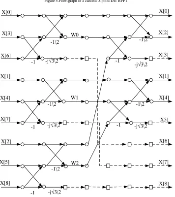
5.4 Canonic Computations for Compound Size canonic RFFT

In this part, canonic RFFT calculation for any compound size is presented. An N-point RFFT is assumed which is composed of AB-point RFFTs at the main stage and BA-point RFFTs at the second stage, i.e., N = A×B. 4 distinct cases are considered as; N = A ,

Case 1) A is odd, B is odd:

(7)

26

ISSN : 2319-6319 -1\2

-j√3\2 -1

X[0]

X[1]

X[2]

X[0]

X[1]

X[2]

Figure 5.Flow-graph of a canonic 3-point DIT RFFT

X[0]

X[3]

X[6]

X[1]

X[4]

X[7]

X[2]

X[5]

X[8]

-1

-1\2

-j√3\2

-1

-1\2

-j√3\2

-1\2

-1

-j√3\2

-1

-1\2

-j√3\2

-1

-1\2

-j√3\2

X[0]

X[2]

X[3]

X[1]

X[4]

X5]

X[6]

X[7]

X[8]

W0

W1

W2

Figure 6. Flow-graph of a canonic 9-point DIT RFFT

(8)

27

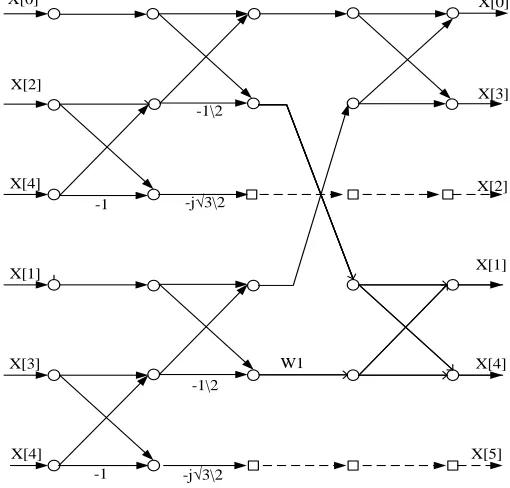
ISSN : 2319-6319 If A is odd and B is even, samples can be deleted from the B-point FFT whose inputs are all purely real. As an example let A=3(odd) and B=2(EVEN) so N=3×2=6.The 6-point canonic RFFT is constructed by using 3-point RFFT. The 6-point RFFT is as shown in figure 7.

X[0]

X[2]

X[4]

X[1]

X[3]

X[4]

X[0]

X[3]

X[2]

X[1]

X[4]

X[5] -1

-1

-1\2

-1\2 -j√3\2

-j√3\2

W1

Case 3) A is even, B is odd;

If A is even and B is odd, then , samples can be deleted. As an example let A=2(even) and B=3(odd) so N=2×3=6.The 6-point canonic RFFT is constructed by using 2 and 3-point RFFT. The 6-point RFFT is as shown in figure 8.

X[0]

X[3]

X[1]

X[4]

X[2]

X[5]

X[0]

X[1]

X[2]

X[3]

X[4]

X[5] -1

W1

Case 4) A is even, B is even;

This case covers all radix-2m RFFT structures. As an example, let A=4(even) and B=4(even) then N=4×4=16.A radix-4 16-point RFFT is shown in figure 4.

(9)

28

ISSN : 2319-6319 All the architectures are modeled in Verilog HDL and synthesized using ISE-Xilinx tool. All the designs were synthesized using Spartan FPGA. Table 1. show the synthesis results of conventional RFFT and canonic RFFT with respect to the area in terms of number of LUTs, path delay and power consumption.

Table-1 Comparison between convention RFFT and canonic RFFT.

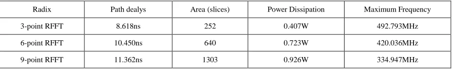
Table 2 shows the synthesis results of 3-piont,6-point,9-point canonic RFFT with respect to the area in terms of number of LUTs, path delay and power consumption.

Table 2.Comparison between different point canonic RFFT.

Radix Path dealys Area (slices) Power Dissipation Maximum Frequency

3-point RFFT 8.618ns 252 0.407W 492.793MHz

VII. CONCLUSION

This paper has designed RFFT architectures using canonic sign digit multiplier and carry select adder. As where the number of signal values calculated at each intermediate FFT stage is same as the size of RFFT so the designed FFT is called as canonic and as the given input is real so called as RFFT. It is shown that canonic RFFT architectures require less twiddle factor operations than the conventional RFFT. Canonic RFFT architecture uses less power and area as compared to the conventional RFFT.

REFERENCES

[1] H. V. Sorensen, D. L. Jones, M. Heideman, and C. S. Burrus, “Real-valued fast fourier transform algorithms,” IEEE Transactions on Acoustics, Speech and Signal Processing, vol. 35, No. 6, pp. 849–863, 1987.

[2] J. W. Cooley and J. W. Tukey, An Algorithm for the Machine Computationof Complex Fourier Series, Mathematics Computation, Vol. 19,pp. 297-301, April 1965.

[3] M. Garrido, K. K. Parhi, and J. Grajal, “A pipelined FFT architecture for real-valued signals,” IEEE Transactions on Circuits and Systems I: Regular Papers, Vol. 56, No. 12, pp. 2634–2643, 2009.

[4] M. Ayinala and K. K. Parhi, “Parallel-Pipelined radix-22_{FFT architecture for real valued signals,” in}_{Proc. Asilomar Conf. Signals, Syst.}

Comput., 2010, pp. 1274–1278.

[5] S. A. Salehi, R. Amirfattahi, and K. K. Parhi, “Pipelined architectures for real-valued FFT and hermitian-symmetric IFFT with real datapaths,” IEEE Transactions on Circuits and Systems II: Express Briefs, vol. 60,no. 8, pp. 507–511, 2013.

[6] M. Ayinala and K. K. Parhi, “FFT architectures for real-valued signals based on radix-23_{and radix-2}4_{algorithms,” IEEE Transactions on}

Circuits and Systems I: Regular Papers, vol. 60, no. 9, pp. 2422–2430,2013.

[7] Prabir Saha, A. Banerjee, I. Banerjee, and A. Dandapat “High Speed Low Power Floating Point Multiplier Design Based On CSD (Canonical Sign Digit)”VDAT 2012

[8] R. M. Hewlitt and E. S. Swartzlantler ”Canonical signed digit representation for FIR digital filters” Signal Processing Systems, 2000. SiPS 2000. 2000 IEEE Workshop on

[9] I-Chyn Wey,Cheng-Chen Ho,Yi-Sheng Lin and Chien-Chang Peng”An Area-Efficient Carry Select Adder Design by Sharing the Common Boolean Logic Term” Proceeding of IMECS 2012 Vol II,Hong Kong

[10] V. Oppenheim, R. W. Schafer, and J. R. Buck, Discrete-time signal processing. Prentice-hall Englewood Cliffs, 1989. [11] Megha Parhi, Yingjie Lao, Keshab K. Parhi” Canonic Real-Valued FFT Structures” Asilomar 2014.

Conventional RFFT Canonic RFFT

Parameters 4-Point RFFT

8-Point RFFT

16-Point RFFT

4-Point RFFT

8-Point RFFT

16-Point RFFT

Number of LUTs 448 718 2289 287 536 1976

Path delay 7.795ns 11.831ns 13.490ns 5.589ns 8.795ns 11.130ns