Study and analysis of quality of service in different
image based steganography using Pixel Mapping
Method (PMM)
Souvik Bhattacharyya
Department of CSE University Institute of Technology,
The University of Burdwan West Bengal, India
Gautam Sanyal
Department of CSE National Institute of Technology,
Durgapur West Bengal, India
ABSTRACT
In this work authors investigate the performance of state of the art Pixel Mapping Method (PMM) an image based steganography method proposed in the literature. This method is tested against a number of well-known image similarity metrics operate in the spatial domain. All the experiments are performed based on the large data set of PMM based stego images generated at different domain. This image data set is categorized with respect to size, quality and texture to determine their potential impact on various steganalysis performance also. To establish a comparative evaluation of techniques, some undetected results obtained at various embedding rates plays a vital role. In addition to variation in cover and stego image properties, the comparison also takes into consideration different message length definitions and computational complexity issues.
Keywords
Cover Image, Pixel Mapping Method (PMM), Stego Image, BPCS (Bit Plane Complexity Segmentation), Integer wavelet domain.
1.
INTRODUCTION
To protect secret message from being stolen during trans-mission, there are two ways to solve this problem in general. One way is encryption, which refers to the process of en-coding secret information in such a way that only the right person with a right key can decode and recover the original information successfully. Another way is steganography and this is a technique which hides secret information into a cover media or carrier so that it becomes unnoticed and less attractive. Capacity and invisibility are the benchmarks needed for data hiding techniques of steganography. A famous illustration of steganography is Simmons’ Prisoners’
Problem [21].An assumption can be made based on this model is that if both the sender and receiver share some common secret information then the corresponding steganography protocol is known as then the secret key steganography where as pure steganography means that there is none prior information shared by sender and receiver. If the public key of the receiver is known to the sender, the steganographic protocol is called public key steganography [2], [3] and [12].For a more thorough knowledge of steganography methodology the reader may see [18], [24].Some Steganographic model with high security features has been presented in [4], [5] and [6].Almost all digital file formats can be used for steganography, but the image and audio files are more suitable because of their high degree of redundancy [24]. Fig. 1 below shows the different categories
of steganography techniques.
Fig 1: Types of Steganography
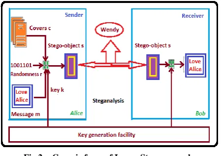
A block diagram of a generic image steganographic system is given in Fig. 2.
Fig 2: Generic form of Image Steganography
A message is embedded in a digital image (cover image) through an embedding algorithm, with the help of a secret key. The resulting stego image is transmitted over a channel to the receiver where it is processed by the extraction algorithm using the same key. During transmission the stego image, it can be monitored by unauthenticated viewers who will only notice the transmission of an image without discovering the existence of the hidden message.
Rest of the paper has been organized as following sections: Section II describes some related works, Section III describes the Pixel Mapping Method in brief. Various performance measure parameters are discussed in Section IV. Experimental results are shown in Section V. Section VI contains the computation complexity analysis of the embedding procedures in various domain and Section VII draws the conclusion.
2.
RELATED
WORKS
ON
IMAGE
STEGANOGRAPHY
IN
SPATIAL
DOMAIN
In this section various steganography based data hiding methods namely LSB, PVD, GLM and the methodology pro-posed by Ahmad et al. has been discussed.
2.1
Data Hiding by LSB
Various techniques about data hiding have been proposed in literatures. One of the common techniques is based on manipulating the least-significant-bit (LSB) [9], [11] and [16], [20] planes by directly replacing the LSBs of the cover-image with the message bits. LSB methods typically achieve high capacity but unfortunately LSB insertion is vulnerable to slight image manipulation such as cropping and compression.
2.2
Data Hiding by PVD
The pixel-value differencing (PVD) method proposed by Wu and Tsai [26] can successfully provide both high embed-ding capacity and outstanding imperceptibility for the stego-image. The pixel-value differencing (PVD) method segments the cover image into non overlapping blocks containing two connecting pixels and modifies the pixel difference in each block (pair) for data embedding. A larger difference in the original pixel values allows a greater modification. In the extraction phase, the original range table is necessary. It is used to partition the stego-image by the same method as used to the cover image. Based on PVD method, various approaches have also been proposed. Among them Chang et al. [15]. proposes a new method using tri-way pixel-value differencing which is better than original PVD method with respect to the embedding capacity and PSNR.
2.3
Data Hiding by GLM
In 2004, Potdar et al. [13] proposes GLM (Gray level modification) technique which is used to map data by modifying the gray level of the image pixels. Gray level modification Steganography is a technique to map data (not embed or hide it) by modifying the gray level values of the image pixels. GLM technique uses the concept of odd and even numbers to map data within an image. It is a one-to-one mapping between the binary data and the selected pixels in an image. From a given image a set of pixels are selected based on a mathematical function. The gray level values of those pixels are examined and compared with the bit stream that is to be mapped in the image.
Fig 3: Data Embedding Process in GLM
Fig 4: Data Extraction Process in GLM
2.4
Data Hiding by the method proposed
by Ahmad T et al.
In this work [1] a novel Steganographic method for hiding information within the spatial domain of the grayscale image has been proposed. The proposed approach works by dividing the cover into blocks of equal sizes and then embeds the message in the edge of the block depending on the number of ones in left four bits of the pixel.
3.
PIXEL MAPPING METHOD (PMM)
Bhattacharyya and Sanyal proposed a new image trans-formation technique in [7], [23] known as Pixel Mapping Method (PMM), a method for information hiding within the spatial domain of an image. Embedding pixels are selected based on some mathematical function which depends on the pixel intensity value of the seed pixel and its 8 neighbors are selected in counter clockwise direction. Before embedding a checking has been done to find out whether the selected embedding pixels or its neighbors lies at the boundary of the image or not. Data embedding are done by mapping each two or four bits of the secret message in each of the neighbor pixel based on some features of that pixel. Figure 5 and Figure 6 shows the mapping information for embedding two bits or four bits respectively.
Fig 5: PMM Mapping Technique for embedding of two bits
Extraction process starts again by selecting the same pixels required during embedding. At the receiver side other different reverse operations has been carried out to get back the original information.
3.1
PMM based BPCS Steganography in
Gray Scale Image
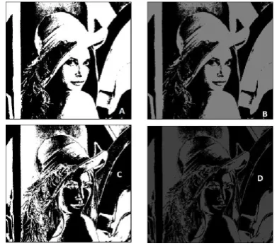
robustness and similarity measures between cover image and stego image. Figure 7 shows various bit planes of Lena image before and after embedding of message.
Fig 6: PMM Mapping Technique for embedding of four bits
Fig 7: A) Bit Plane 1 of Lena before embedding B) Bit Plane 1 of Lena after embedding C) Bit Plane 2 of Lena before embedding D) Bit Plane 2 of Lena after embedding.
3.2
PMM in Wavelet Domain
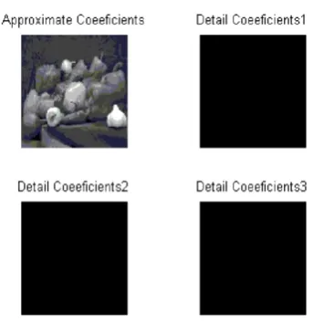
This is an image based steganography method for information hiding in discrete integer wavelet domain of gray scale image. The input messages can be in any digital form, and are often treated as a bit stream. This approach works by converting the gray level image in transform domain using discrete integer wavelet technique through lifting scheme [8], [17] and [19].This approach performs a 2-D lifting wavelet decomposition through Haar lifted wavelet of the cover image and computes the approximation coefficients matrix CA and detail coefficients matrices CH, CV, and CD. Next step is to apply the PMM [7], [23] technique for 2 bit embedding in those coefficients for embedding the secret message and then apply inverse transformation on those wavelet coefficients to form the stego image. Embedded wavelet coefficients are selected based on some mathematical function which depends on the intensity value of the seed coefficient and its 8
neighbors are selected in counter clockwise direction. Before embedding a checking has been done to find out whether the randomly selected wavelet coefficients or its neighbor lies at the boundary of the image or not. Extraction process starts again by selecting the same wavelet coefficients required during embedding. At the receiver side other different reverse operation has been carried out to get back the original information. Figure 8 and 9 shows the level 1 decomposition of Lena and Pepper image.
Fig 8: Level 1 Wavelet Decomposition of Lena
4.
VARIOUS PERFORMANC METRICS
FOR EVALUATING THE RESULTS
For measuring the performance of Pixel Mapping Method in various domains like Gray Scale, Colour, Bit Plane and Wavelet various image similarity calculation metrics like MSE,RMSE,PSNR,SSIM,KL divergence distances and Normalized Cross-correlation has been incorporated. Besides stego images produced by the various versions of the proposed algorithm has been tested through well known steganalysis attack namely RS analysis and Chi-square analysis.4.1
Mean Squared Error (MSE), Root
Mean Squared Error (RMSE) and Peak
Signal to Noise Ratio (PSNR)
the stego-image, i.e. it measures the percentage of the stego data to the image percentage.
Fig 9: Level 1 Wavelet Decomposition of Pepper
The root-mean-square deviation (RMSD) or root-mean-square error (RMSE) is a frequently used measure of the differences between values predicted by a model or an estimator and the values actually observed from the thing being modeled or estimated. RMSD is a good measure of accuracy. These individual differences are also called residuals, and the RMSD serves to aggregate them into a single measure of predictive power.
The PSNR is used to evaluate the quality of the stego-image after embedding the secret message in the cover. Assume a cover image C (i,j) that contains N by N pixels and a stego image S(i,j) where S is generated by embedding / mapping the message bit stream. Mean squared error (MSE) of the stego image is calculated as equation 1.
2
(1)
The PSNR is computed using the following formulae given in Equation 2:
PSNR = 10 log
10255
2/ MSE db.
(2)4.2
Structural Similarity (SSIM)
The structural similarity (SSIM) [27] index is a method for measuring the similarity between two images. The SSIM index is a full reference metric, in other words, the measuring of image quality based on an initial uncompressed or distortion-free image as reference. SSIM is designed to improve on traditional methods like peak signal-to-noise ratio (PSNR) and mean squared error (MSE), which have proved to be inconsistent with human eye perception.
The SSIM metric is calculated on various windows of an image. The measure between two images x and y of common size N x N is:
Where the average of , is the average of , the
variance of , the variance of , the covariance of
and , , two variables to stabilize the division with weak denominator. is the dynamic range of the pixel-values and and by default.
4.3
Kullback Leibler Divergence
In probability theory and information theory, the Kullback-Leibler Divergence [10] (also information divergence, information gain, relative entropy, or KLIC) is a non-symmetric measure of the difference between two probability distributions P and Q. KL measures the expected number of extra bits required to code samples from P when using a code based on Q, rather than using a code based on P. Typically P represents the ”true” distribution of data, observations, or a precisely calculated theoretical distribution. The measure Q typically represents a theory, model, description, or approximation of P. Although it is often intuited as a metric or distance, the KL divergence is not a true metric for example, it is not symmetric: the KL from P to Q is generally not the same as the KL from Q to P. For probability distributions P and Q of a discrete random variable their KL divergence is defined to be
) ( ) ( log ) ( ) || ( i Q i P i P Q PD
KL (4)In words, it is the average of the logarithmic difference between the probabilities P and Q, where the average is taken using the probabilities P. The K-L divergence is only defined if P and Q both sum to 1 and if Q (i) > 0 for any i such that P(i) > 0. If the quantity 0log0 appears in the formula, it is interpreted as zero. For distributions P and Q of a continuous random variable, KL-divergence is defined to be the integral
dx
x
q
x
p
x
p
Q
P
D
KL)
(
)
(
log
)
(
)
||
(
(5)where p and q denote the densities of P and Q. More generally, if P and Q are probability measures over a set X, and Q is absolutely continuous with respect to P, then the Kullback–Leibler divergence from P to Q is defined as
x KLdP
dP
dQ
Q
P
D
(
||
)
log
(6)where
dP
dQ is the Radon–Nikodym derivative of Q with
respect to P, and provided the expression on the right-hand side exists. Likewise, if P is absolutely continuous with respect to Q, then
x x KLdQ
dQ
dP
dQ
dP
dP
dQ
dP
Q
P
D
(
||
)
log
log
(7)which we recognize as the entropy of P relative to Q. Continuing in this case, if μ is any measure on X for
which
d
dP
p
and
d
dQ
q
exist, then the Kullback–Leibler divergence from P to Q is given as
x KL d q p p Q PD ( || ) log
(8)1) Steganography Security using Kullback Leibler Diver-gence: Denoting C the set of all covers c, Cachin’s definition of steganographic security [10] is based on the assumption that the selection of covers from C can be described by a random variable c on C with probability distribution function (pdf) P. A steganographic scheme, S, is a mapping C x M x K → C that assigns a new (stego) object, s ε C, to each triple (c,M,K), where M ε M is a secret message selected from the set of communicable messages, M, and K ε K is the steganographic secret key. Assuming the covers are selected with pdf P and embedded with a message and secret key both randomly (uniformly) chosen from their corresponding sets, the set of all stego images is again a random variable s on C with pdf Q. The measure of statistical detectability is the Kullback Leibler divergence
Stego system is called -secure against passive attackers, ifD (P|| Q) and perfectly secure if = 0.
4.4
Cross Correlation
For comparing the similarity between cover image and the stego image, the normalized cross correlation coefficient (r) has been computed. In statistics, correlation indicates the strength and direction of a linear relationship between two random variables. The correlation coefficient ρxybetween two
random variables X and Y with expected values μx and μy and
standard deviations σx and σy is defined as:
where E is the expected value operator and cov means covariance. The value of correlation is 1 in the case of an increasing linear relationship, -1 in the case of a decreasing linear relationship, and some value in between in all other cases, indicating the degree of linear dependence between the variables. Cross correlation is a standard method of estimating the degree to which two series are correlated. Consider two series x(i) and y(i) where i = 0,1,2,. . . , N-1. The cross correlation r at delay d is defined as
where mx and my are the means of the corresponding series. Similarity measure of two images can be done with the help of normalized cross correlation generated from the above concept using the following formula:
Here C is the cover image, S is the stego image, m1 is the
mean pixel value of the cover image and m2 is the mean pixel
value of stego image.
4.5
Steganalysis of the Stego Images
through Chi-Square Analysis
The majority of steganographic utilities for the camouflage of confidential communication suffer from fundamental weaknesses. On the way to more secure steganographic algorithms, the development of attacks is essential to assess security. Here in this work all the stego images produced by the proposed algorithm has been tested through Chi-square Analysis. Andreas Pfitzmann and Andreas Westfield [25] introduced a method based on statistical analysis of Pair of Values (PoVs) that are exchanged during sequential embedding. This attack works on any sequential embedding type of stego-system such as EzStego and Jsteg. Sequential embedding makes PoVs in the values embedded in. For example, embedding in the spatial domain makes PoVs (2i,2i +1) such that 0 1, 2 3, 4 5, , 252 253, 254 255. This will affect the histogram Yk of the images pixel value k,
while the sum of Y2i + Y2i+1 will remain unchanged. Thus the
expected distribution of the sum of adjacent values given in equation (13) and the value for the difference between distributions with v -1 degrees of freedom as in equation (14). From (13) and (14) we get the 2 statistic for our PoVs as in (15).
Chi-Square Analysis calculates the average LSB and constructs a table of frequencies and Pair of Values [14], It takes the data from these two tables and performs a chi-square test. It measures the theoretical vs. calculated population difference. The Chi-Square Analysis calculates the chi-square value for every 128 bytes of the image. As it iterates through, the chi-square value it calculates becomes more and more accurate until too large of a data set has been produced.
4.6
Computational Complexity
Computational complexity measures is a branch of theoretical computer science and mathematics that focuses on classifying computational problems.
1) Complexity Measures: For solving a problem at a given amount of time and space, computational model like deterministic Turing machine can be used. The time required by a deterministic Turing machine M on input x is the total number of state transitions, or steps, the machine makes before it halts and outputs the answer which may be yes or no. A Turing machine M is said to operate within time f(n), if the time required by M on each input of length n is at most f(n). Any decision problem A solving in time f(n) means there exists a Turing machine operating in time f(n) that solves the problem.
C
c
Q
c
c
P
c
P
Q
P
D
lg
(9) (9)(10)
(11)
2) Best, worst and average case complexity: The best, worst and average case complexity refer to three different ways of measuring the time complexity (or any other complexity measure) of the inputs of the same size. Since some inputs of size n may be faster to solve than others, complexities may be defined as:
Best-case complexity: This is the complexity of solving the problem for the best time for input of size n.
Worst-case complexity: This is the complexity of solving the problem for the worst time for the input of size n.
Average-case complexity: This is the complexity of solving the problem on an average. This complexity is only defined with respect to a probability distribution over the inputs. For instance, if all inputs of the same size are assumed to be equally likely, the average case complexity can be defined with respect to the uniform distribution over all inputs of size n. For example, consider the algorithm of quick sort. The worst-case is when the input is sorted or sorted in reverse order, and the algorithm takes time O(n2) for this case and the average time taken for sorting is O(n log n). The best case occurs when each pivoting divides the list in half, also needing O(n log n) time.
5.
EXPERIMENTAL RESULTS
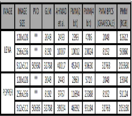
In this section the authors discusses the experimental results of the proposed method in Gray Scale Domain, Colour Domain and Bit Plane Domain based on two benchmarks techniques to evaluate the hiding performance. First one is the capacity of hiding data and another one is the imperceptibility of the stego image, also called the quality of stego image. A comparative study of the proposed methods with some other existing methods like PVD, GLM and the methods proposed by Ahmad T et al. by are also discussed in this section .Experimental results of stego images are computed based on two well known images: Lena and Pepper. Figure 10 shows the comparisons of embedding capacity of PMM in various domains with other existing methods.
5.1
Experimental Results of PMM in Gray
Scale Domain
This section calculates the various performance measure parameters on gray scale domain using 2 bit and 4 bit data embedding method. Fig 11 and Fig 12 shows the calculation of various image similarity metrics for PMM 2 bit and 4 bit embedding for gray scale image.
Fig 10: Comparison of embedding capacity (** For PVD method all the images used are of size 512x512.)
5.2
Experimental Results of PMM (2 bit) in
RGB Domain
This section calculates the various performance measure parameters for PMM based Steganography method for RGB images. Fig 36 shows the calculation of various image similarity metrics for PMM based data embedding for RGB images
5.3
Experimental Results of PMM (2 bit) in
Bit Plane Domain
This section calculates the various performance measure parameters for PMM based BPCS Steganography for gray scale image. Fig 35 shows the calculation of various image similarity metrics for PMM based 2 bit BPCS data embedding for gray scale image. Figure 33 and 34 shows the various results based on the Chi Square Analysis.
5.4
Experimental Results of PMM (2 bit) in
Wavelet Domain
Images Similarity
Parameters LENGTH OF THE EMBEDDING CHARACTER
100 500 1000 2000 5000 10000 20000 40000
Lena 512X512
PSNR 72.3599 65.6221 62.5946 59.3945 55.3362 52.3521 49.3173 46.3159 MSE 0.0038 0.0178 0.0358 0.0748 0.1903 0.3783 0.7609 1.5187 RMSE 0.0509 0.1076 0.1513 0.2181 0.3470 0.4873 0.6904 0.9749 SSIM 1.0 0.99 0.99 0.99 0.9996 0.9993 0.9988 0.9974 Correlation 1.0 1.0 1.0 1.0 0.9999 0.9999 0.9997 0.9995 Entropy 7.55 7.55 7.54 7.54 7.54 7.50 7.50 7.498
KL 7.1815e-006 2.6254e-005 5.0630e-005 1.0817e-004
2.8138e-004 5.4170e-004 0.0018 0.0034
Lena 256X256
PSNR 66.8066 59.3663 56.3423 53.3134 49.3343 46.3312
N.A.
MSE 0.0136 0.0752 0.1510 0.3032 0.7580 1.5134 RMSE 0.0909 0.2210 0.3112 0.4384 0.6873 0.9728 SSIM 0.9999 0.9996 0.99 0.9981 0.9963 0.9915 Correlation 1.0 1.0 0.99 0.9999 0.9999 0.9997 Entropy 7.54 7.54 7.54 7.54 7.54 7.54
KL 1.2996e-005 9.4258e-005 1.8227e-004 3.5437e-004
8.4351e-004 0.0017
Lena 128X128
PSNR 60.42 53.64 50.373 47.3189
N.A. MSE 0.0589 0.2811 0.5959 1.2056
RMSE 0.1898 0.4 0.5954 0.8607 SSIM 0.999 0.998 0.998 0.9964 Correlation 1.0 0.99 0.99 0.9998 Entropy 7.559 7.551 7.53 7.50
KL 5.9706e-005 2.0840e-004 4.9666e-004 0.0012
Pepper 512X512
PSNR 72.9561 65.6119 62.5637 59.4950 55.4277 52.4133 49.3417 46.3185 MSE 0.0033 0.0179 0.0360 0.0730 0.1863 0.3730 0.7567 1.5179 RMSE 0.0478 0.1054 0.1477 0.2098 0.3364 0.4745 0.6764 0.9643 SSIM 1.0000 0.9999 0.9998 0.9997 0.9993 0.9987 0.9974 0.9943 Correlation 1.0000 1.0000 1.0000 1.0000 1.0000 0.9999 0.9998 0.9997 Entropy 6.9828 6.9828 6.9833 6.9835 6.9815 6.9755 6.9522 6.8388
KL 7.5596e-006 2.6307e-005 4.4742e-005 8.5514e-005
2.2067e-004 4.1750e-004 8.4292e-004 0.0018
Pepper 256X256
PSNR 66.4956 59.5031 56.3931 53.4142 49.3246 46.3070
N.A. MSE 0.0146 0.0729 0.1492 0.2962 0.7597 1.5219
RMSE 0.0973 0.2122 0.3056 0.4260 0.6785 0.9666 SSIM 0.9998 0.9992 0.9986 0.9977 0.9940 0.9876 Correlation 1.0000 1.0000 1.0000 0.9999 0.9998 0.9997 Entropy 6.9831 6.9831 6.9819 6.9781 6.9510 6.8368
KL 2.0977e-005 9.1991e-005 1.9669e-004 3.5233e-004
8.3994e-004 0.0018
Pepper 128X128
PSNR 60.56 53.3228 50.3011 47.1909
N.A. MSE 0.057 0.3026 0.6067 1.2416
RMSE 0.1764 0.4320 0.6113 0.8822 SSIM 0.9995 0.995 0.9965 0.9928 Correlation 1.0 0.9999 0.9999 0.9997 Entropy 6.9833 6.9778 6.9617 6.8890 KL 3.9155e-005 3.6851e-004 7.4242e-004 0.0016
Images Similarity Paramete
rs
LENGTH OF THE EMBEDDING CHARACTER
100 500 1000 2000 5000 10000 20000 40000 90000
Lena 512X512
PSNR 63.4131 59.0393 56.3090 52.6683 47.7562 44.5811 41.3445 38.2985 33.8397 MSE 0.0296 0.0811 0.1521 0.3518 1.0901 2.2645 4.7712 9.6212 26.8601 RMSE 0.1597 0.2527 0.3502 0.5375 0.9407 1.3665 1.9943 2.8102 4.9970
SSIM 0.9999 0.9997 0.9995 0.9992 0.9985 0.9958 0.9925 0.9859 0.9678 Correlati
on 1.0000 1.0000 0.9999 0.9999 0.9996 0.9992 0.9984 0.9969 0.9929 Entropy 7.0876 7.0871 7.0858 7.0821 7.0766 7.0703 7.0295 6.8974 5.9759
KL Div
5.3793e-005 1.8084e-004 3.7315e-004 7.9555e-004 0.0021 0.0046 0.0098 0.0195 0.0372
Lena 256X256
PSNR 55.6428 49.7924 47.0365 43.8901 39.9249 36.8699 34.0024 NA NA MSE 0.1773 0.6821 1.2866 2.6550 6.6160 13.3686 25.8724 NA NA RMSE 0.4042 0.7944 1.0904 1.5721 2.4842 3.5308 4.9202 NA NA SSIM 0.9990 0.9960 0.9951 0.9909 0.9778 0.9609 0.9081 NA NA Correlati
on 1.0000 0.9999 0.9998 0.9995 0.9989 0.9980 0.9964 NA NA Entropy 7.5674 7.5584 7.5543 7.5422 7.4501 7.1948 6.5456 NA NA
KL Div
1.4275e-004 6.4135e-004 0.0012 0.0027 0.0069 0.0144 0.0275 NA NA
Lena 128X128
PSNR 50.5581 43.9064 40.9106 37.8253 NA NA NA NA NA MSE 0.5718 2.6451 5.2725 10.7287 NA NA NA NA NA RMSE 0.7124 1.5585 2.2059 3.1532 NA NA NA NA NA SSIM 0.9990 0.9940 0.9889 0.9803 NA NA NA NA NA Correlati
on 0.9999 0.9995 0.9991 0.9983 NA NA NA NA NA Entropy 7.5551 7.5327 7.4726 7.3062 NA NA NA NA NA
KL Div
4.5017e-004 0.0025 0.0053 0.0111 NA NA NA NA NA
Pepper 512X512
PSNR 62.7029 56.8478 53.8542 50.7937 46.8371 43.9838 41.1036 38.876 33.8662 MSE 0.0349 0.1344 0.2677 0.5416 1.3470 2.5984 5.0433 10.843 26.6970 RMSE 0.1344 0.3132 0.4282 0.6183 1.0010 1.3937 1.9105 2.976 4.9058
SSIM 0.9997 0.9992 0.9987 0.9975 0.9948 0.9900 0.9823 0.9850 0.9349 Correlati
on 1.0000 1.0000 0.9999 0.9999 0.9997 0.9994 0.9988 0.9956 0.9949 Entropy 6.9836 6.9848 6.9867 6.9899 6.9956 6.9928 6.9690 6.7086 5.9302
KL Div
5.1643e-006 1.5981e-004 2.8938e-004 6.4178e-004 0.0018 0.0035 0.0065 0.0140 0.0292
Pepper 256X256
PSNR 58.1571 50.6060 47.7516 45.0902 40.9560 38.3255 35.1660 NA NA MSE 0.0994 0.5656 1.0912 2.0140 5.2177 9.5616 19.7918 NA NA RMSE 0.2047 0.6285 0.8885 1.2241 1.9332 2.6730 3.8830 NA NA SSIM 0.9990 0.9957 0.9924 0.9876 0.9717 0.9527 0.9058 NA NA Correlati
on 1.0000 0.9999 0.9997 0.9995 0.9988 0.9979 0.9957 NA NA Entropy 6.9849 6.9905 6.9941 6.9926 6.9703 6.8602 6.4551 NA NA
KL Div
-2.1884e-005 5.8225e-004 0.0013 0.0028 0.0064 0.0138 0.0289 NA NA
Pepper 128X128
PSNR 51.9206 44.9174 42.1761 39.2010 35.1657 NA NA NA NA MSE 0.4178 2.0958 3.9398 7.8160 19.7928 NA NA NA NA RMSE 0.5398 1.2111 1.6719 2.3757 3.8759 NA NA NA NA SSIM 0.9970 0.9875 0.9815 0.9695 0.9294 NA NA NA NA Correlati
on 0.9999 0.9995 0.9991 0.9982 0.9957 NA NA NA NA Entropy 6.9900 6.9962 6.9799 6.9124 6.4621 NA NA NA NA
KL Div
4.8842e-004 0.0025 0.0049 0.0104 0.0286 NA NA NA NA
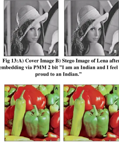
Fig 13:A) Cover Image B) Stego Image of Lena after embedding via PMM 2 bit ”I am an Indian and I feel
proud to an Indian.”
Fig 14: A) Cover Image B) Stego Image of Pepper after embedding via PMM (RGB) 2 bit ”I am an Indian
and I feel proud to an Indian.”
6.
COMPUTATIONAL COMPLEXITY
ANALYSIS FOR PMM
Computational complexity of the proposed embedding method has been calculated using the graphical plot between the Embedding Data Size vs. Computation Time. From the plot a polynomial relation between the two parameter has been formed using the curve fitting algorithm. Fitness algorithm has been evaluated and finally computational complexity has been calculated using the best fitted results. Figure 21, 22 and 23 shows various results related to computation complexity calculation for PMM (2 bit) for Lena (512x512) image. Figure 24, 25 and 26 shows various results related to computation complexity calculation for PMM (4 bit) for Lena (512x512) image. The results of PMM method for RGB image has been shown in figure 27,28 and 29 where as figure 30, 31 and 32 shows various results related to computation complexity calculation for PMM based BPCS (2 bit) method for Lena (512x512) gray scale image.
6.1
Case 1: LENA (512x512) image for
PMM 2bit
1) Linear Polynomial model with 95% confidence bounds for formulating a relation between Computation Time and Data Embedding Size
T (n) = p1 * n + p2 (14) where p1 = 0.02473 and p2 = -63.38
Goodness of fit SSE: 8.198e+004, R-square: 0.9102, Adjusted R-square: 0.8952 and RMSE: 116.9.
2) Quadratic Polynomial model with 95% confidence bounds for formulating a relation between Computation Time and Data Embedding Size
T (n) = p1 * n2 + p2 * n + p3 (15)
where p1 = 7.108e-007, p2 = -0.002594 and p3 = 15.81 Goodness of fit SSE: 7.911e+004, R-square: 0.9656, Adjusted R-square: 0.9607 and RMSE: 106.3
Option 2 (Equation 15) is better fitted and thus the computational complexity PMM 2 bit data embedding procedure is calculated as O(n2)
6.2
Case 2: LENA (512x512) image for
PMM 4bit
1) Linear Polynomial model with 95% confidence bounds for formulating a relation between Computation Time and Data Embedding Size
T (n) = p1* n + p2 (16)
where p1 = 0.01772 and p2 = -72.72, Goodness of fit SSE: 1227, R-square: 0.8922, Adjusted R-square: 0.8854 and RMSE: 8.758.
2) Quadratic Polynomial model with 95% confidence bounds for formulating a relation between Computation Time and Data Embedding Size
T (n) = p1* n2 + p2*n + p3 (17)
where p1 = 1.395e-007, p2 = 0.00567 and p3 = -5.675 Goodness of fit SSE: 1032, R-square: 0.9996, Adjusted R-square: 0.9994 and RMSE: 13.11.
Option 2 (Equation 17) is better fitted and thus the computational complexity for data embedding procedure is calculated as O(n2)
6.3
Case 3: Pepper (512x512) image for
PMM based BPCS (2bit)
1) Linear Polynomial model with 95% confidence bounds for formulating a relation between Computation Time and Data Embedding Size
T (n) = p1* n + p2 (18)
where p1 = 0.0002831 and p2 = 1.185, Goodness of fit SSE: 10.24, R-square: 0.9219, Adjusted R-square: 0.9132 and RMSE: 1.066.
2) Quadratic Polynomial model with 95% confidence bounds for formulating a relation between Computation Time and Data Embedding Size
T (n) = p1* n2 + p2* n + p3 (19)
where p1 = 1.009e-008, p2 = -2.261e-005 and p3 = 2.062, Goodness of fit SSE: 0.6512,R-square: 0.995,Adjusted R-square: 0.9938 and RMSE: 0.2853.
6.4
Case 4: LENA (512x512) image for
PMM based BPCS (2bit)
1) Linear Polynomial model with 95% confidence bounds for formulating a relation between Computation Time and Data Embedding Size
T (n) = p1* n + p2 (20)
where p1 = 0.0002587, p2 = -1.286 Goodness of fit SSE: 9.003, R-square: 0.9181, Adjusted R-square: 0.909 and RMSE: 1.
2) Quadratic Polynomial model with 95% confidence bounds for formulating a relation between Computation Time and Data Embedding Size
T (n) = p1 * n2 + p2 * n + p3 (21)
where p1 = 9.371e-009, p2 = -2.521e-005 and p3 = 2.101, Goodness of fit SSE: 0.7357, R-square: 0.9933, Adjusted R-square: 0.9916 and RMSE: 0.3032.
Option 2 (Equation 21) is better fitted and thus the computational complexity for data embedding procedure is calculated as O(n2)
Fig 15: Embedding capacity of the PMM Wavelet Method
Fig 16: PSNR value after embedding through PMM Wavelet Method in Approximate Coefficients (CA) of
Lena (256x256)
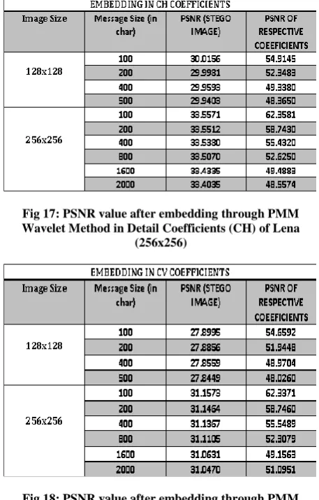
Fig 17: PSNR value after embedding through PMM Wavelet Method in Detail Coefficients (CH) of Lena
(256x256)
Fig 18: PSNR value after embedding through PMM Wavelet Method in Detail Coefficients (CV) of Lena
(256x256)
Fig 19: PSNR value after embedding through PMM Wavelet Method in Detail Coefficients (CD) of Lena
(256x256)
7.
CONCLUSION
PMM for RGB) is much better compared to other existing methods. With the computation of various image similarity metrics as shown in various figures for measuring the similarity between the cover image and stego image, this method gives an excellent result. From the security aspects of the hidden data the relative entropy distance (KL divergence) is very low between the cover image and stego image which yields a very high security value of the hidden data. Results of image and stego image which yields a very high security value of the hidden data. From the result of Chi-Square test it can be seen statistical and probability distribution plot of the cover image and stego images of various embedding capacity for PMM based BPCS steganography are same which concludes that hidden message stays undetected for Chi-Square analysis in PMM based BPCS Steganography Technique.PMM based method for integer wavelet can avoid some image attack like noise addition also.
Fig 20: Noise Attack on PMM method in Wavelet Domain
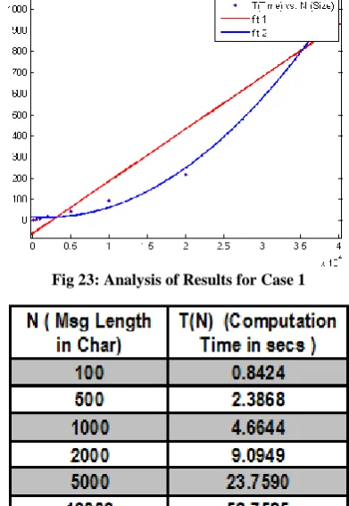
Fig 21: Computation Time at various embedding length for Lena 512 (Case 1)
Fig 22: Plot of Computation Time at various embedding length for Lena 512 (Case1)
Fig 23: Analysis of Results for Case 1
Fig 24: Computation Time at various embedding length for Lena 512 (Case 2)
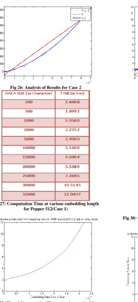
Fig 26: Analysis of Results for Case 2
Fig 27: Computation Time at various embedding length for Pepper 512(Case 1)
Fig 28: Plot of Computation Time at various embedding length for Pepper 512 (Case 1)
Fig 29: Analysis of Results for Case 1
Fig 30: Computation Time at various embedding length for Lena 512 (Case 2)
Fig 32: Analysis of Results for Case 2
8.
REFERENCES
[1] Ahmad T. Al-Taani. and Abdullah M. AL-Issa. A novel steganographic method for gray-level images. International Journal of Computer, Information, and Systems Science, and Engineering, 3, 2009.
[2] RJ Anderson. Stretching the limits of steganography. Information Hiding, Springer Lecture Notes in Computer Science, 1174:39–48, 1996.
[3] Ross J. Anderson. and Fabien A.P.Petitcolas. On the limits of steganography. IEEE Journal on Selected Areas in Communications (J-SAC),Special Issue on Copyright and Privacy Protection, 16:474–481, 1998.
[4] Souvik Bhattacharyya. and Gautam Sanyal. Study of secure steganography model. In Proceedings of International Conference on Advanced Computing and Communication Technologies (ICACCT-2008),Panipath,India, 2008.
[5] Souvik Bhattacharyya. and Gautam Sanyal. An image based steganography model for promoting global cyber security. In Proceedings of International Conference on Systemics, Cybernetics and Informatics, Hyderabad, India, 2009.
[6] Souvik Bhattacharyya. and Gautam Sanyal. Implementation and design of an image based steganographic model. In Proceedings of IEEE International Advance Computing Conference, Patiala, India, 2009.
[7] Souvik Bhattacharyya. and Gautam Sanyal. Hiding data in images using pixel mapping method (pmm). In Proceedings of 9th annual Conference on Security and Management (SAM) under The 2010 World Congress in Computer Science, Computer Engineering, and Applied Computing(World Comp 2010), LasVegas,USA, July 12-15,2010.
[8] Geert Uytterhoeven Dirk Roose Adhemar Bultheel. Integer wavelet transforms using the lifting scheme. In CSCC Proceedings, 1999.
[9] J.Y. Hsiao. C.C. Chang. and C.-S. Chan. Finding optimal least significant-bit substitution in image hiding by dynamic programming strategy. Pattern Recognition, 36:1583–1595, 2003.
[10]Cachin. An information theoretic model for steganography. Proceedings of 2nd Workshop on
Information Hiding. D. Aucsmith (Eds.).Lecture Notes in Computer Sciences, Springer-verlag., 1525, 1998. [11]C.K. Chan. and L. M.Cheng. Hiding data in images by
simple lsb substitution. Pattern Recognition, 37:469–474, 2004.
[12]Scott. Craver. On public-key steganography in the presence of an active warden. In Proceedings of 2nd International Workshop on Information Hiding., pages 355–368, Portland,Oregon, USA, 1998.
[13]Potdar V.and Chang E. Gray level modification steganography for secret communication. In IEEE International Conference on Industria lInformatics., pages 355–368, Berlin, Germany, 2004.
[14]Guillermito. Steganography: A few tools to discover hidden data. 2004.
[15]P Huang. K.C. Chang., C.P Chang. and T.M Tu. A novel image steganography method using tri-way pixel value differencing. Journal of Multimedia, 3, 2008.
[16]Y. K. Lee. and L. H.Chen. High capacity image steganographic model.IEE Proc.-Vision, Image and Signal Processing, 147:288–294, 2000.
[17]W. Sweldens. The lifting scheme. A construction of second generation wavelets. SIAM J. Math. Anal., 29:511–546, 1997.
[18]N.F.Johnson. and S. Jajodia. Steganography: seeing the unseen. IEEE Computer, 16:26–34, 1998.
[19]W. Sweldens R. Calderbank, I. Daubechies and B.L. Yeo. Wavelet transforms that map integers to integers. Appl. Comput. Harmon. Anal.,5:332–369, 1998. [20]C.F. Lin. R.Z. Wang. and J.C. Lin. Image hiding by
optimal lsb substitution and genetic algorithm. Pattern Recognition, 34:671–683,2001.
[21]Gustavus J. Simmons. The prisoners’ problem and the subliminal channel. Proceedings of CRYPTO., 83:51–67, 1984.
[22]Aparajita Khan et al. Souvik Bhattacharyya and Gautam Sanyal. Pixel mapping method (pmm) based bit plane complexity segmentation (bpcs) steganography. In Proceedings of WICT 2011, Mumbai ,India, 2011. [23]Lalan Kumar Souvik Bhattacharyya and Gautam Sanyal.
A novel approach of data hiding using pixel mapping method (pmm). INTERNATIONAL JOURNAL OF COMPUTER SCIENCE AND INFORMATION SECURITY (IJCSIS), 8, 2010.
[24]JHP Eloff. T Mrkel. and MS Olivier. An overview of image steganography. In Proceedings of the fifth annual Information Security South Africa Conference., 2005. [25]Andreas Westfeld and Andreas Pfitzmann. Attacks on
steganographic systems. In Proceedings of the Third Intl. Workshop on Information Hiding, Springer-verlag., pages 61–76, 1999.
[26]D.C. Wu. and W.H. Tsai. A steganographic method for images by pixel value differencing. Pattern Recognition Letters, 24:1613–1626, 2003.
[27]IEEE Alan Conrad Bovik Fellow IEEE Hamid Rahim Sheikh Student Member IEEE Zhou Wang, Member and IEEE. Eero P. Simoncelli, Senior Member. Image quality assessment: From error visibility to structural similarity. IEEE TRANSACTIONS ON IMAGE PROCESSING.,
Images LENGTH OF THE EMBEDDING CHARACTER
100 500 1000 5000 10000 20000 32000
Lena 512X512
PSNR 76.1778 69.2907 66.2363 59.3224 53.8742 45.2285 36.6817 MSE 0.0016 0.0077 0.0155 0.0760 0.2665 1.9509 13.9607 RMSE 0.0322 0.0684 0.0978 0.2170 0.4100 1.1272 3.0312
SSIM 1.0000 1.0000 1.0000 0.9999 0.9995 0.9966 0.9698 Correlation 1.0000 1.0000 1.0000 1.0000 0.9999 0.9993 0.9951 KL divergence 0.01646 0.0404 0.1952 0.1001 0.6018 0.0090 0.3997 Entropy 7.0879 7.0880 7.0879 7.0873 7.0851 7.0733 7.0506
Lena 256X256
PSNR 70.0117 63.2014 60.2652 45.282 NA NA NA MSE 0.0065 0.0311 0.0612 1.9269 NA NA NA RMSE 0.0623 0.1382 0.1941 1.1221 NA NA NA SSIM 1.0000 0.9998 0.9997 0.9899 NA NA NA Correlation 1.0000 1.0000 1.0000 0.9997 NA NA NA
KL divergence 0.0088 0.0501 0.0273 0.0031 NA NA NA Entropy 7.5682 7.5680 7.5675 7.5505 NA NA NA
Lena 128X128
PSNR 64.3532 57.2843 49.4810 NA NA NA NA
MSE 0.0239 0.1215 0.7328 NA NA NA NA
RMSE 0.1220 0.2742 0.6880 NA NA NA NA
SSIM 0.9999 0.9996 0.9976 NA NA NA NA Correlation 1.0000 1.0000 0.9999 NA NA NA NA KL divergence 0.04154 0.0553 0.1792 NA NA NA NA Entropy 7.5598 7.5553 7.5433 NA NA NA NA
Pepper 512X512
PSNR 76.3612 69.2627 66.2783 59.3220 53.5295 44.3295 35.6439 MSE 0.0015 0.0077 0.0153 0.0760 0.2885 2.3996 17.7293 RMSE 0.0310 0.0699 0.0982 0.2165 0.4228 1.2148 3.2563
SSIM 1.0000 1.0000 0.9999 0.9997 0.9989 0.9928 0.9562 Correlation 1.0000 1.0000 1.0000 1.0000 0.9999 0.9995 0.9960 KL divergence 0.0132 0.0176 0.9809 0.0411 0.1017 0.0019 0.0601 Entropy 6.9829 6.9830 6.9835 6.9832 6.9820 6.9365 6.8194
Pepper 256X256
PSNR 70.3187 63.2984 60.2815 44.340 NA NA NA MSE 0.0060 0.0304 0.0609 2.3935 NA NA NA RMSE 0.0581 0.1354 0.1933 1.2057 NA NA NA SSIM 0.9999 0.9997 0.9995 0.9821 NA NA NA Correlation 1.0000 1.0000 1.0000 0.9995 NA NA NA KL divergence 0.0232 0.0537 0.0319 0.0018 NA NA NA Entropy 6.9831 6.9836 6.9825 6.9338 NA NA NA
Pepper 128X128
PSNR 64.2544 57.1638 49.6043 NA NA NA NA
MSE 0.0244 0.1249 0.7123 NA NA NA NA
RMSE 0.1230 0.2773 0.6725 NA NA NA NA
SSIM 0.9998 0.9993 0.9962 NA NA NA NA Correlation 1.0000 1.0000 0.0011 NA NA NA NA KL divergence 0.0499 0.0670 0.0854 NA NA NA NA Entropy 6.9824 6.9799 6.9633 NA NA NA NA
57