Analysis of Machining Parameters of Endilling Cutter on Surface
Roughness for Aa 6061-T6
Katara Hiren
1, Kadam Priyanaka
2, Vanshika Shukla
3,
Mr. Parth Shah
41-3UG Student, Mechanical Engineering Dept.,Sigma Institute Of Engineering,Vadodara,Gujarat,India
4Assistant Professor, Mechanical Engineering Dept.,Sigma Institute Of Engineering,Vadodara,Gujarat,India
ABSTRACT
End milling is the most commonly used milling operation. This experiment consist of numerous end milling operation on a work piece with varying different parameters like speed, feed and depth of cut. After that Analysis of Variance (ANOVA) was done on the design expert software using response surface method of design of experiment (DOE) to find out which of the parameters amongst speed, feed and depth of cut have a greater impact on surface roughness. We observed speed have a greater impact on surface roughness.
Key words: end milling, ANOVA, speed, feed, depth of cut, surface roughness.
I. INTRODUCTION
End milling cutter are used in milling machines to perform milling operations. Milling cutters remove material by their movement within machine. The dynamic behaviour of the milling operation can lead to unstable cutting conditions. The present work focuses on effect of machining parameters on surface roughness. The good the surface quality the better the machining so it is important to study the parameters which has a greater effect on surface finish. There are many parameters which affect the quality of surface obtained. End milling is one of the important material cutting process in a production industry. We can do multiple types of cutting like peripheral cutting, face milling end milling. A good surface leads to better performance of
milling cutter and it is also resistive to corrosion. The machining parameters have a greater effect on the quality of the surface obtained.
II. METHODS AND MATERIAL
Fig: [1] work piece
The tool used in the experiment was made up of solid carbide. Cutter because this tool material combines increased stiffness with the ability to operate at higher RPM. Carbide tools are best suited for shops operating newer milling machines or machines with minimal spindle wear. Rigidity is critical when using carbide tools. these material also provides good surface finish on the work piece. These tool material can cut harder
surface and have a good tool life.
Figure: [2] endmill cutter.
The experiment was carried out with different machining conditions to analyze the effect of speed, feed and depth of cut by taking 27 different
conditions including 3 speed*3feed*3 depth of cut. The experiment was performed on VMC 640i
manufactured by Jyoti laboratories. Three speeds selected in RPM were250,500 and 750 and feeds in mm/min were 100,200 and 300. The depth of cuts in mm were 0.5,1 and 1.5. Response Surface
Method was used for assignment of the factors and surface roughness in micron was response variable. The roughness test was performed on portable surface roughness tester, Model: SJ-201P,
Make: mitutoyo, Sr.No.:310397
III. RESULTS AND DISCUSSION
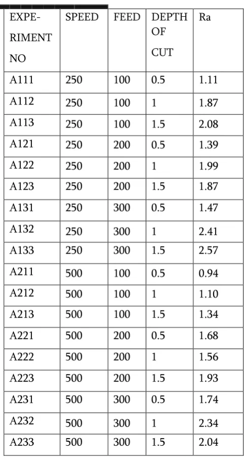
We got the values of surface roughness test for different machining conditions after the surface roughness test which are as shown in table 1. The values are in the range of 0.86 micron to 2.57 micron. After this ANOVA analysis was carried out on Design Expert Software 11.
Table no. 2 shows the results of Anova. Here, The Model F-value of 20.77 implies the model is significant. There is only a 0.01% chance that an F-value this large could occur due to noise and P-values less than 0.0500 indicate model terms are significant. In this case A, B, C are significant model terms. Values greater than 0.1000 indicate the model terms are not significant. If there are many insignificant model terms (not counting those required to support hierarchy), model reduction may improve your model. The Lack of Fit F-value of 3.22 implies the Lack of Fit is significant. There is only a 4.98% chance that a Lack of Fit F-value this large could occur due to noise. Significant lack of fit is bad -- we want the model to fit.
Table 3 shows the fit statistics in that the Predicted R² of 0.6353 is in reasonable agreement with the Adjusted R² of 0.6953; i.e. the difference is less than 0.2. Adequate Precision measures the signal to noise ratio. A ratio greater than 4 is desirable. Your ratio of 14.334 indicates an adequate signal. This model can be used to navigate the design space.
Table 4 shows the model comparison statistics
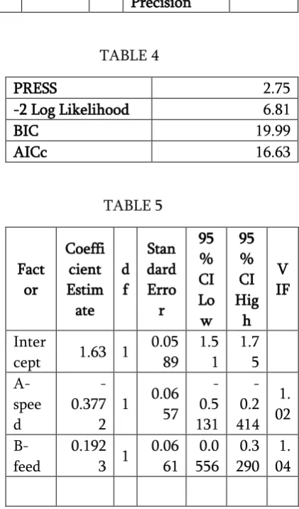
Table 5 show Coefficients in Terms of Coded Factors. The coefficient estimate represents the expected change in response per unit change in factor value when all remaining factors are held
constant. The intercept in an orthogonal design is the overall average response of all the runs. The coefficients are adjustments around that average based on the factor settings. When the factors are orthogonal the VIFs are 1; VIFs greater than 1 indicate multi-colinearity, the higher the VIF the more severe the correlation of factors. As a rough rule, VIFs less than 10 are tolerable.
TABLE 1
EXPE-
RIMENT
NO
SPEED FEED DEPTH
OF
CUT
Ra
A111 250 100 0.5 1.11
A112 250 100 1 1.87
A113 250 100 1.5 2.08
A121 250 200 0.5 1.39
A122 250 200 1 1.99
A123 250 200 1.5 1.87
A131 250 300 0.5 1.47
A132 250 300 1 2.41
A133 250 300 1.5 2.57
A211 500 100 0.5 0.94
A212 500 100 1 1.10
A213 500 100 1.5 1.34
A221 500 200 0.5 1.68
A222 500 200 1 1.56
A223 500 200 1.5 1.93
A231 500 300 0.5 1.74
A232 500 300 1 2.34
A311 750 100 0.5 0.86
A312 750 100 1 1.11
A313 750 100 1.5 1.O2
A321 750 200 0.5 1.39
A322 750 200 1 1.74
A323 750 200 1.5 1.88
A331 750 300 0.5 0.96
A332 750 300 1 1.12
A333 750 300 1.5 1.25
TABLE 2 Sourc e Sum of Squar es D f Mea n Squa re F-val ue p-valu e Mode
l 5.51 3 1.84
20. 77 < 0.00 01 signific ant
A-speed 2.92 1 2.92
32. 99 < 0.00 01 B-feed 0.748
8 1
0.74 88 8.4 7 0.00 79
C-doc 1.12 1 1.12 12.
70 0.00
17 Resid
ual 2.03
2 3
0.08 85 Lack
of Fit 1.75
1 5 0.11 64 3.2 2 0.04 98 signific ant Pure Error 0.288
8 8
0.03 61 Cor
Total 7.55
2 6
TABLE 3
Std.
Dev. 0.2974 R² 0.7304
Mean 1.58 Adjusted R² 0.6953
C.V. % 18.88 Predicted R² 0.6353
Adeq
Precision 14.3341
TABLE 4
PRESS 2.75
-2 Log Likelihood 6.81
BIC 19.99
AICc 16.63
TABLE 5 Fact or Coeffi cient Estim ate d f Stan dard Erro r 95 % CI Lo w 95 % CI Hig h V IF Inter
cept 1.63 1
0.05 89 1.5 1 1.7 5 A-spee d -0.377 2
1 0.06
57 -0.5 131 -0.2 414 1. 02 B-feed 0.192
3 1
0.06 61 0.0 556 0.3 290 1. 04
they are spread in a normal distribution.
Fig: [4] Normal plot of residuals
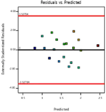
Figure 5 shows the residual vs predicted plot there is no specific pattern . Analysis of the residual plots, it can be established that there is no uncertain changes between the residuals and predicted values we can see that the residuals have a constant variance and hence the developed model is highly significant and can be used for the prediction.
Fig: [5] Residual vs Predicted
Figure 4 is the plot of the residuals versus run, we can see that there is not any pattern above or below 0.
Fig : [6] Residual vs Run
Figure 7 shows the predicted versus the actual graph.
Fig :[7] Predicted vs Actual
IV. CONCLUSION
V. REFRENCES
1. G Boothroyd and W. Knight: Fundamentals of
Machining and Machine Tools. Second Edition, Marcel Dekker Inc., New York. 1989. 2. P Balakrishnan and M. F. De Vries: Analysis
of Mathematical Model building Techniques Adaptable to Machinability Data Base System, Proceeding
3. E M. Trent: Metal Cutting,
Butterworth-Heinemann Ltd., Oxford. England, 1991. 4. V P. Astakhov and M. O Osman: Journal of
Materials Processing Technology, vol. 62, No 3, 1996, 175-179.
5. Giunta et al., 1996; van Campen et al., 1990, Toropov et al., 1996.
6. N Tabenkin: Carbide and Tool, vol. 21, 1985.
12-15 .g of NAMRC-XI, 1983.
7. Parth shah: Investigation on Surface
Roughness of AA 6061-T6 for End Milling,IJSTE, Volume 2 | Issue 10 | April 2016 ISSN (online): 2349-78 pg 687-690
8. Parth Shah;Investigation on surface roughness