An Enhanced Run Length Encoding using an Elegant Pairing Function for Medical Image Compression

(1)

An Enhanced Run Length Encoding using an Elegant Pairing

Function for Medical Image Compression

Adolfo Solís-Rosas1, Sandra Luz Canchola-Magdaleno2 and Ma. Teresa García-Ramírez3

1, 2, 3 _{Faculty of Informatics, Autonomous University of Querétaro, Santiago de Querétaro, Querétaro 76230,} México

1_{[email protected],}2_{[email protected],}3_{[email protected]}

ABSTRACT

Medical image compression is in high demand in the medical field, since it reduces the required time to transmit an image in a bandwidth or store an image for medical purposes. Modern medical image diagnostics involves a large set of medical images that are often based on MRI, X-Rays or CT. However, the introduction of new technologies and the fast development of existing ones has resulted in a high demand for bandwidth. In this article, the proposed image compression method for medical images it uses the discrete wavelet transform as a compression tool, which provides a better compression ratio without losing valuable information and through the implementation of the proposed enhanced run length encoder, by the use of the elegant pairing function, we can achieve higher compression ratios and high visual quality. Despite this, the fidelity is subject to the capabilities and limitations of the Human Visual System.

Keywords: Medical Image Compression, DWT, RLE, Elegant Pairing Function, Lossy Image Compression, Entropy Coding.

1. INTRODUCTION

Human vision is one of the most advanced and important senses for humans, therefore, digital images have a strong impact on human perception. The interest in digital image processing emerges from two application areas: improving graphic information for human interpretation and processing graphic information for storage purposes [1].

Currently, given the high demand for multimedia applications and the continuous development of new technologies, transmitting graphic information has resulted in a lack of bandwidth in a transmission channel and has made it difficult to store this kind of

graphic information [2]. Therefore, the theory of data compression has come to have a strong impact on reducing the data redundancy to save more storage space and facilitating transmission bandwidth [3]. The theory of image compression requires an understanding of Shannon’s information theory. Shannon’s metric is called “Entropy” which is the amount of information contained in a variable [4]. This information is determined, among other things, by the number of different values that variable can take, the number of bits required to store the variable, the absolute minimum amount of storage and transmission needed [5]. For every possible state exists a set of probabilities ( ) of producing different possible symbols . Thus, there is an entropy for each state. The Eq. 1 defines the entropy of the source.

∑

( )

(1)

(2)

Fig. 1. Architecture Of The Proposed Image Compression Method

Medical digital images have a fundamental importance in the perception and visualization of medical information that

leads to an effective medical diagnosis [6]. However, medical analysis produces a large quantity of medical graphic information which leads to a challenge in storing and transmitting the great volume of data [7]. The aim of image compression is reducing the volume of data through a data compression method that permits a higher compression ratio without losing the most important visual details allowing an effective medical diagnosis [7].

There are two types of compression methods, lossless and lossy image compression:

 Lossless: The numerical reconstruction of the compressed image is identical to the original image.

 Lossy: This method has high compression ratios at the expense of degrading the information, resulting in a visual deformation of the compressed image. The loss of information is proportional to the compression ratio achieved.

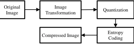
A general image compression scheme consists of three fundamental parts: removing coding redundancy, removing correlation between pixels of the image and removing the psycho visual redundancy, which is the data ignored by the human visual system [8]. Image compression systems that combine lossless and lossy schemes are known as hybrid coding. The general architecture of a lossy image compression scheme is shown in Fig. 2.

Fig. 2. General Lossy Image Compression Scheme.

This paper is organized as follows: the first section introduces a brief description of the topic, the second section explains the method used in this paper for medical image compression, the third section presents

experimental results. Finally, our conclusions are presented in fourth section.

2. THE PROPOSED METHOD

The objective of the proposed method in this research paper is to present an efficient and effective lossy compression scheme for medical digital images. The proposed method it uses the DWT to reduce the psycho visual redundancy. Therefore, the main contribution of this research project is to ameliorate the entropy coding process which removes coding redundancy. As a result, coding redundancy is removed by the Run Length Encoding process. In order to improve the compression ratio of the image we utilized a paring function to code every tuple of the entropy coding process. Fig. 2 describes the process of the proposed image compression method.

2.1 Discrete Wavelet Transform

A wavelet is an orthogonal function which can be applied to a discrete set of data. The DWT of a signal decomposes the image into subband components. The DWT is used for image compression, the use of the DWT gives better reconstructed images and high compression ratios at lower bit rates. DWT covers both frequency and time information [9]. To use wavelets for digital image compression, the rows and columns of the matrix that represents the image have to be scanned and transformed to generate the wavelet coefficients. The mother wavelet  has the basis shape created by a scaling function  “average” low-pass filter and a wavelet function  “difference” high-pass filter [10].

The first step is to pass the samples through a low pass filter then they have to be passed through a high pass filter and next apply convolution to both coefficients. After getting the filter coefficients the coefficients have to be down sampled by 2, and the process must be repeated. The results are an approximation and detail coefficients [11]. Fig. 3 shows the 1-D DWT.

Original Image

Image

Transformation Quantization

(3)

Fig. 3. Decomposition process for the 1-D DWT.

In order to generate the wavelet coefficients, the rows and columns of the image have to be scanned. The decomposed signal can be reconstructed again into the original signal using reconstruction filters, which are the inverse of the decomposition filters. The Eq. 2 is used to generate the wavelet coefficients.

( ) ∑

∑

( ) ( ) (

)

∑

( ) ( ) ( )

∑

( ) ( ) ( )

∑

( ) ( ) ( )

2)

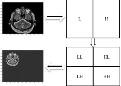
The output came from high-pass filter (H) and low-pass filter (L), the image is decomposed into four parts: LL, HH, LH, HL. Where LL is the sum of the vertical low-pass filter and the horizontal high-pass filter, HH is the sum of the horizontal high-pass filter and the vertical high-pass filter, LH is the sum of the horizontal low-pass filter and the vertical high-pass filter, HL is the sum of the horizontal high-pass filter and the vertical low-pass filter [12]. Fig. 4 illustrates the 1-level wavelet decomposition applied to a medical image.

Fig. 4. Single level wavelet decomposition applied to an image.

The wavelet filter banks are constructed from different wavelet basis functions such as Haar, Daubechies, Symlets, Coiflets and Biorthogonal. However, the selection of the best wavelet function depends on the requirements and the application of the process [13]. Due to the fact that current compression systems use biorthogonal wavelet instead of orthogonal wavelets, the proposed method uses biorthogonal wavelets. One wavelet filter is used to decompose the original signal and another wavelet filter is used to reconstruct the signal [14]. Fig. 5 presents the Biorthogonal Wavelet PSI for a) decomposition and b) reconstruction.

a) b)

Fig. 5. Biorthogonal Wavelet PSI for a) decomposition and b) reconstruction.

2.2 Quantization

The quantization process consists of defining a threshold to quantize all the wavelet coefficients. This process makes compression lossy; the objective is to create a sparse matrix reducing the bits to store the transformed image and mapping float numbers to integer numbers. All the values with magnitude less than the threshold are quantized to zero, creating a sparse matrix [15]. The quantization step is used through the uniform scalar quantization, this function is given by Eq. 3.

( ) {

⌊

( )

⌋

⌊

( )

⌋

₍₃₎

2.3 Entropy Coding

After the transformation and quantization process, the image is represented by a set of integer numbers, many of them are zeros. In order to encode the quantized coefficients to represent a more compact image, the transformed matrix is mapped to a

vector. This process is named ZigZag Scanning. Fig. 6 represents the ZigZag Scanning process.

0 0.5 1

-1 0 1Desc Wavelet PSI bior1.1

0 2 4 6

-1 0 1 Desc Wavelet PSI bior1.3

0 5 10

-1 0 1

Desc Wavelet PSI bior1.5

0 2 4 6

0 5 10

0 5 10 15 -2 0 2

0 1 2 3

-100 0 100Desc Wavelet PSI bior3.1

0 2 4 6 -5

0 5Desc Wavelet PSI bior3.3

0 5 10

-2 0 2

0 0.5 1

-1 0 1Reco Wavelet PSI bior1.1

0 2 4 6

0 5 10

0 2 4 6

-1 0 1 2Reco Wavelet PSI bior2.2

0 5 10

-1 0 1 Reco Wavelet PSI bior2.4

0 5 10 15 -1 0 1

Reco Wavelet PSI bior2.6

0 1 2 3

-1 0 1 Reco Wavelet PSI bior3.1

0 2 4 6 -1

0 1Reco Wavelet PSI bior3.3

0 5 10

-1 0 1Reco Wavelet PSI bior3.5 Origina l Data High pass filter Low pass filter 2 2 Approximate coefficients Detail coefficient s

L H

LL HL

(4)

Fig. 6. ZigZag Scan of the coefficients of the single level wavelet decomposition of a 2-D image.

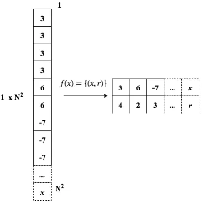
The coefficients with low frequencies are going in the top of the vector and the coefficients with high frequencies are going in the bottom of the vector. The ZigZag Scanning allows a high run length of zeros in the vector [16]. The run length encoding process encodes every coefficient denoted by of the vector of coefficients ( ) , creating a matrix of

, where is the number of different nonconsecutive elements. Fig. 7 illustrates the encoding process by run length encoding.

Fig. 7. Entropy coding by Run Length Encoding process.

2.3 Elegant Pairing Function

A pairing function is a unique and a bijective function. It is a function that maps a pair of coordinates , where * + denotes the nonnegative integer numbers. Every point on a surface can be described by a pair of coordinates. When x and y are nonnegative integer numbers, the elegant pair function associates these numbers and outputs a single nonnegative integer number that is uniquely associated with that pair. The elegant pairing function assigns consecutive numbers to

points along the edge of squares [15]. Fig. 8 illustrates the elegant pairing function.

Fig. 8. The elegant pairing function. Source: Adapted from [17].

2.3 Enhanced Run Length Encoding

To achieve higher compression ratios, the proposed method encodes the run length encoding matrix through a pairing function. Because a pairing function is a unique and a bijective function, it is possible to recover the data without losing information as seen in Eq. 4.

(4)

To encode two elements of a coordinates pair, the pairing function associates these two numbers with a unique nonnegative number, this function is described as follows in Eq. 5.

(5)

Due to the nature of the wavelet coefficients, it is possible to have negative numbers, so we proposed a modified elegant pairing function in order to achieve higher compression ratios. Eq. 6 shows the modified version of the elegant pairing function * + :

{

_{( )}

{

_{( )}

( ) {

(6)

Therefore, the proposed method for decoding through the elegant pairing function it is defined on Eq. 7

* +

{

* ⌊√ ⌋

⌊√ ⌋

(5)

{

_{( )}

{

_{( )}

7

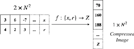
The enhanced run length encoding process using the modified elegant pairing function it is illustrated in the Fig. 9.

Fig. 9. Illustrative encoding process using the elegant pairing function.

Now one can observe a compressed image in the form of a bitstream. This new, compressed image is easier to store and transmit. It is not possible to have a visual representation of the image. The decompression process is the inverse process of the compression method, because every part of the compression method has an inverse process and the result is a reconstructed image with high visual quality.

3. EXPERIMENTAL RESULTS

For the purpose of evaluating the performance of a compression algorithm, it is necessary to define metrics that estimate the quality of the compressed image and the difference between the original image and the reconstructed image. This difference is commonly named distortion. The performance of a compression algorithm will be good if the distortion criteria is small, the smaller the distortion, the higher the quality of the reconstructed image. We used various comparison parameters associated with medical image compression:

3.1 MSE

The Mean Squared Error (MSE) is based on approximating the measures of the distortion to determine the quality of the reconstructed image as seen in Eq. 8. The lower the value of MSE, the lower the error.

( )

∑ ∑(

)

8)

3.2 PSNR

The PSNR measure represents the Peak Signal to Noise Ratio. It denotes the fidelity between the

original image and the reconstructed image. The higher the PSNR value, the better the quality of the compressed image as presented in Eq. 9. The PSNR value is measured in decibels (dB).

(

( ))

(9)

3.3 SSIM

The Structural Similarity Index (SSIM) it is a well-known metric to measure the similarity between two images. This metric considers the correlation with the perception of the Human Visual System. It models the distortion of the image based on the correlation, luminance and contrast distortion as shown in Eq. 10.

( ) ( ) ( ) ( )

where,

{

( )

₍₁₀₎

The positive values of the SSIM metric are in the range of , -. A value of means no correlation between the original and reconstructed image, and value of 1 means .

3.4 Compression Ratio

The compression ratio (CR) it is defined as the ratio of the size of the original image to the size of the compressed image as seen in Eq. 11.

(11)

3.5 Simulation Results

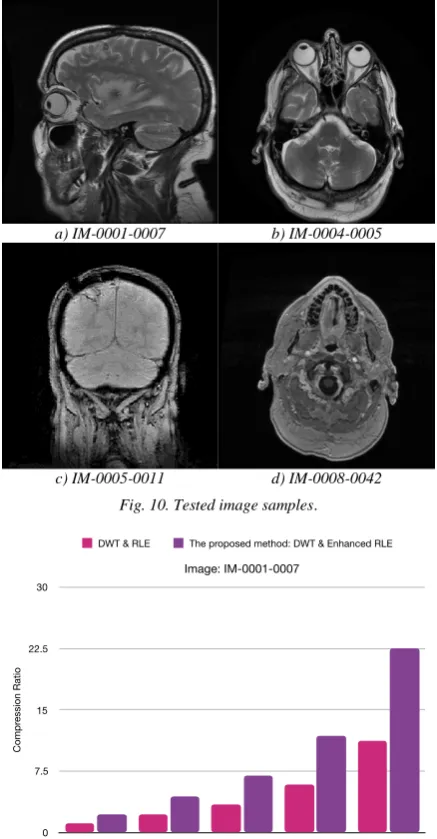
The proposed medical image compression method is implemented in MATLAB R2018a. Fig. 10 illustrates the four medical test images on which the proposed method was implemented. Fig. 11, Fig. 12, Fig. 13 and Fig. 14 present a comparison of the different compression ratios acquired in the proposed method against a typical lossy image compression method based on the DWT and run length encoding as entropy coder. Table 1 shows the execution time and the different compression quality metrics defined in the previous section of the proposed method by the use of the DWT and an enhanced run length encoding using different quantization values.

(6)

a) IM-0001-0007 b) IM-0004-0005

c) IM-0005-0011 d) IM-0008-0042

Fig. 10. Tested image samples.

Fig. 11. Comparison of different compression ratios obtained from test image IM-0001-0007.

(7)

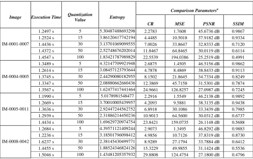
Table 1: Experimental Results of the Proposed Method

Image Execution Time Quantization

Value Entropy

Comparison Parametersa

CR MSE PSNR SSIM

IM-0001-0007

1.2497 s 5 5.30487488693298 2.2783 1.7608 45.6736 dB 0.9867 1.2524 s 15 3.86120417742194 4.4485 10.5018 37.9182 dB 0.9334 1.4436 s 30 3.13701069099555 7.0026 33.8647 32.8333 dB 0.7120 1.4372 s 50 2.52748676202014 11.8467 64.8465 30.0119 dB 0.6114 1.4547 s 100 1.83421787989829 22.5539 194.0386 25.2519 dB 0.4991

IM-0004-0005

IM-0005-0011

IM-0008-0042

Comparison parameters based on Eq. 8, 9, 10, 11

The proposed method does not affect the quality of the recovered image, since the entropy coding process is a lossless compression method. Observing Fig. 11, Fig. 12, Fig. 13 and Fig. 14 we conclude that through the implementation of the elegant pairing function in the run length encoding process, we can achieve higher compression ratios without losing the most important visual details of the image, yielding in an effective medical diagnosis. Also based on the results of the Table 1, we see that the quality of the reconstructed image is satisfactory. The desired visual quality of the image is subject to the Human Visual System.

3. CONCLUSIONS

This paper provides an architecture for medical image compression by the discrete wavelet transform, an enhanced entropy coding based on run length encoding and a pairing function. The proposed method is performed on different MRI images and is a hybrid compression method. The higher the threshold on the quantization process, the higher the compression ratio and the higher the loss of information this means a lesser entropy value. Our proposed method can be used for future research. Also, the experimental results show that the use of the

elegant pairing function upon the run length encoder can achieve higher compression ratios without losing information, making for a more effective medical diagnosis and ready for store or transmission purposes.

ACKNOWLEDGMENTS

I want to acknowledge the financial support for this research work to the “Consejo Nacional de Ciencia y Tecnología” (CONACYT) through the scholarship with number 494037.

REFERENCES

[1] R. C. Gonzalez and R. E. (Richard E. Woods, Digital image processing. 2008.

[2] A. Alarabeyyat et al., “Lossless Image Compression Technique Using Combination Methods,” J. Softw. Eng. Appl., vol. 05, no. 10, pp. 752–763, 2012.

[3] W.-Y. Wei, “An introduction to image processing,” Opt. Lasers Eng., vol. 15, no. 4, pp. 281–282, Jan. 2008.

(8)

[5] S. Vajapeyam, “Understanding Shannon ’ s Entropy metric for Information,” Arxiv, no. March, pp. 1–6, 2014.

[6] H. Amri, A. Khalfallah, M. Gargouri, N. Nebhani, J.-C. Lapayre, and M.-S. Bouhlel, “Medical Image Compression Approach Based on Image Resizing, Digital Watermarking and Lossless Compression,” J. Signal Process. Syst., vol. 87, no. 2, pp. 203–214, May 2017.

[7] A. J. Hussain, A. Al-Fayadh, and N. Radi, “Image compression techniques: A survey in lossless and lossy algorithms,” Neurocomputing, vol. 300, pp. 44–69, 2018.

[8] M. Vaishnav, C. Kamargaonkar, and M. Sharma, “Medical Image Compression Using Dual Tree Complex Wavelet Transform and Arithmetic Coding Technique,” Int. J. Sci. Res. Comput. Sci. Eng. Inf. Technol., vol. 3, no. 3, pp. 172–176, 2017. [9] E. Tim, “Discrete Wavelet Transforms : Theory and Implementation Tim Edwards ( [email protected] ),” no. September 1991, pp. 1– 26, 1992.

[10] H. R. Mahadevaswamy, “Lossless Image Compression Using Wavelets,” 2000.

[11] R. Patel, “Lossless DWT Image Compression using Parallel Processing,” Indian J. Sci. Technol. ISSN, no. 929, pp. 974–6846, 2016. [12] J. Patil and S. Patil, “Image Compression by DWT and DTCWT Using an SPIHT Algorithm,” Int. J. Sci. Eng. Appl. Sci., vol. 1, no. 6, pp. 321–326, 2015.

[13] A. M. Al-Busaidi, L. Khriji, F. Touati, M. F. A. Rasid, and A. Ben Mnaouer, “Real-time DWT-based compression for wearable Electrocardiogram monitoring system,” 2015 IEEE 8th GCC Conf. Exhib. GCCCE 2015, no. February, 2015.

[14] M. Chaudhary and A. Dhamija, “A BRIEF STUDY OF VARIOUS WAVELET FAMILIES AND COMPRESSION TECHNIQUES,” J. Glob. Res. Comput. Sci., vol. 4, no. 4, 2013.

[15] J. W. & S. D. Sundararajan, “Chapter 15 Image Compression 15 . 1 Lossy Image Compression,” vol. 1, 2015.

[16] D. Sundararajan, “Discrete Wavelet Transform : A Signal Processing Approach,” vol. 1, 2018.

(9)

An Enhanced Run Length Encoding using an Elegant Pairing Function for Medical Image Compression