Biomedical Prediction of Radial Size of Powdered
Element using Artificial Neural Network
Yaagyanika Gehlot1, Bhairvi Sharma1, P Muthu1,*, Hariharan Muthusamy1 and S.Latha2
1Department of Biomedical Engineering, India.
2Department of Electronics and Communication Engineering, India.
SRM Institute of Science and Technology, Kattankulathur, Chennai, Tamil Nadu, India. *Corresponding author E-mail: [email protected]
http://dx.doi.org/10.13005/bpj/1526
(Received: 26 January 2018; accepted: 13 September 2018)
Silver nitrous aqueous solution is used to biosynthesize Silver nanoparticles (Ag-NPs) through a green and easy way using tuber powder extracts of Curcuma Longa (C. longa). The aim is to model an Artificial Neural Network (ANN) using seven existing algorithms in MATLAB for forecasting the size of the silver nanoparticle with volume of both C. longa extraction and AgNO3, time of stirring and temperature of reaction as input functions. Several techniques including Quasi-Newton, Conjugate Gradient and Levenberg-Maquardt are employed for training the designed ANN model, a feed-forward backpropagation network with different combinations of architecture and transfer functions. Each algorithm is fashioned to obtain the best performance by calculating the Regression (R), Mean Square Error (MSE), Mean Absolute Error (MAE) and Error Sum of Squares (SSE), thereby comparing the results and propounding the optimum algorithm technique for the discussed application in nanoengineering. Finally, based on the findings, the optimum network is proposed through the simulation results.
Keywords: Artificial Neural Network, Feed-forward back propagation, Learning Algorithms, Nanoengineering, Silver nanoparticles.
THE Nanoparticles (NPs) are a broad class of materials including particulate substances having a dimension less than 100 nm at least1. Noble metals like Silver in metal Nanoparticles mainly have been used for experimental purposes because of their robust properties in optics. This creates large amount of applications in areas such as photography, dentistry, electronics, food industries, clothing etc2. The shape and size of metal nanoparticle is measured typically using discrete techniques such as Scanning Electron
Microscopy, Transmission Electron Microscopy etc3.
In the last decade an increasing use of artificial intelligence tools was observed in nanotechnology research. Artificial Intelligence can be used in classification of material properties of nanoscale, designing, simulation, nanocomputing etc4. Artificial neural network (ANN) is an efficient as well as dynamic simulation tool which allows one to classify, predict or estimate relationships among inputs and outputs2. They can expertly
Published by Oriental Scientific Publishing Company © 2018
solve difficult problems such as stock exchange prediction, image compression, face recognition etc. These tasks may be carried out without any prior information.
Artificial neural network
An ANN is a computational technique that uses the assistance of a learning paradigm along with processing nodes and attempts to present an affiliation between the input and output data5. Majorly, there are two learning paradigms that an ANN can employ; supervised learning and unsupervised learning6.
A basic ANN network comprises of three primitive layers; input layer, hidden layer and output layer as illustrated in Fig. 1. These layers contain various mathematical functions, nodes which are also called artificial neurons, associated with weights or coefficients that builds the structure of the neural network7. When an input and the corresponding target is provided to the ANN model (the training in this case is supervised), the error is calculated from the difference between the system output and the target response. This information of the error is fed back (Back propagation or BP learning) during the training phase and consequently the weights are adjusted accordingly, thereby improving the system parameters. Reiteration is done until the desired performance is achieved8.
Several types of ANNs have been designed with different configurations either with a single-layer or multiple layer neurons. A multilayer perceptron (MLP) is the best model for complex problems. By introducing more number of hidden layers a MLP outlives the drawback of the single-layer perceptron. In a conventional feed-forward MLP network, the input responses are multiplied
with the weights and these multiplied signals from each input are then summed and guided to a transfer function which gives the output result for that particular neuron7.
Learning algorithms
There are several types of training algorithms that can be adopted to train an ANN. MATLAB provides 9 different types of algorithms for an Engine Data Set problem, out of which top 7 algorithms are explored in this study.
Conjugate Gradient
Conjugate Gradient (CG) starts by searching the negative of the descent in their first iteration. Before the next search is determined, a line search is implemented for acquiring the prime distance to travel forth the existing search direction, so that the two search directions are conjugate. The novel search direction is determined when the new steepest descent direction and the preceding search direction are combined9. Several versions
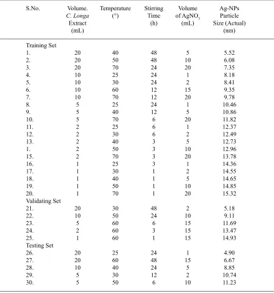
Table 1. Experimental Values For Prediction Of The Size Of Ag-nps
S.No. Volume. Temperature Stirring Volume Ag-NPs C. Longa (°) Time of AgNO3 Particle
Extract (h) (mL) Size (Actual)
(mL) (nm)
Training Set
1. 20 40 48 5 5.52
2. 20 50 48 10 6.08
3. 20 70 24 20 7.35
4. 10 25 24 1 8.18
5. 10 30 24 2 8.41
6. 10 60 12 15 9.35
7. 10 70 12 20 9.78
8. 5 25 24 1 10.46
9. 5 40 12 5 10.86
10. 5 70 6 20 11.82
11. 2 25 6 1 12.37
12. 2 30 6 2 12.49
13. 2 40 3 5 12.73
1. 2 50 3 10 12.96
15. 2 70 3 20 13.78
16. 1 25 3 1 14.36
17. 1 30 1 2 14.55
18. 1 40 1 5 14.65
19. 1 50 1 10 14.85
20. 1 70 1 20 15.32
Validating Set
21. 20 30 48 2 5.18
22. 10 50 24 10 9.11
23. 5 60 6 15 11.69
24. 2 60 3 15 13.47
25. 1 60 1 15 14.93
Testing Set
26. 20 25 24 1 4.90
27. 20 60 48 15 6.67
28. 10 40 24 5 8.85
29. 5 30 12 2 10.74
30. 5 50 6 10 11.23
of CG are determined by computational means of the constant, ²k6.
Powell/Beale Restarts (traincgb)
Powell/Beale (CGB) technique will restart if the current and previous gradient have very little orthogonality between them9.
Fletcher-Reeves Update (traincgf)
For the Fletcher-Reeves Update (CGF), the constant is calculated as the ratio of the norm squared of the present gradient to the norm squared of the previous gradient7.
Polak-Ribiére Update (traincgp)
Another practice of the CG algorithm is Polak-Ribiére Update (CGP). In CGP, the constant is calculated by the inner product of the previous gradient change with the current gradient divided by the norm squared of the previous gradient. CGP requires more storage than CGF6.
Scaled Conjugate Gradient (trainscg)
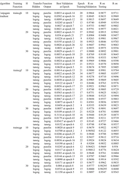
Table 2. Results And Comparison Of Algorithms Using Different Architectures And Transfer Functions
Algorithm Training H Transfer Function Best Validation Epoch R on R on R on Function Hidden Output at Epoch Training Validation Testing
Conjugate traincgb 10 logsig purelin 0.0033 at epoch 14 20 0.9864 0.9877 0.9711 Gradient logsig logsig 0.0582 at epoch 16 22 0.8845 0.9633 0.9969 logsig tansig 0.0099 at epoch 12 18 0.9815 0.9697 0.9649 tansig purelin 0.0245 at epoch 7 13 0.9740 0.8949 0.9554 tansig logsig 0.0027 at epoch 7 13 0.9753 0.9807 0.9802 tansig tansig 0.0021 at epoch 10 16 0.9791 0.9977 0.8021 20 logsig purelin 0.0022 at epoch 31 37 0.9942 0.9915 0.9942 logsig logsig 0.054 at epoch 21 27 0.8904 0.9408 0.9457 logsig tansig 0.0226 at epoch 3 9 0.9263 0.9901 0.9967 tansig purelin 0.0195 at epoch 12 18 0.9925 0.8846 0.9703 tansig logsig 0.0026 at epoch 26 32 0.9687 0.9941 0.9043 tansig tansig 0.0031 at epoch 7 13 0.9855 0.9975 0.9556 30 logsig purelin 0.0029 at epoch 11 17 0.9800 0.9892 0.9901 logsig logsig 0.0053 at epoch 10 25 0.8769 0.9189 0.9645 logsig tansig 0.0439 at epoch 4 10 0.9556 0.9353 0.9667 tansig purelin 0.0024 at epoch 34 40 0.9969 0.9886 0.9398 tansig logsig 0.0233 at epoch 15 21 0.9521 0.8570 0.9058 tansig tansig 0.0620 at epoch 5 11 0.9674 0.7895 0.9405 traincgf 10 logsig purelin 0.0014 at epoch 15 21 0.9880 0.9981 0.9784 logsig logsig 0.0022 at epoch 28 34 0.9077 0.9805 0.8597 logsig tansig 0.0376 at epoch 12 18 0.9278 0.9710 0.9496 tansig purelin 0.0030 at epoch 22 28 0.9905 0.9869 0.9605 tansig logsig 0.0122 at epoch 7 13 0.8446 0.9763 0.9576 tansig tansig 0.0056 at epoch 17 23 0.9921 0.9963 0.9871 20 logsig purelin 0.0021 at epoch 11 17 0.9748 0.9805 0.9729 logsig logsig 0.0563 at epoch 11 17 0.8751 0.9625 0.8621 logsig tansig 0.0419 at epoch 17 23 0.9844 0.9325 0.9494 tansig purelin 0.0067 at epoch 17 23 0.9694 0.9557 0.9883 tansig logsig 0.0075 at epoch 5 11 0.8501 0.9856 0.9855 tansig tansig 0.0456 at epoch 2 8 0.9355 0.9439 0.9823 30 logsig purelin 0.0057 at epoch 6 12 0.9776 0.9891 0.9697 logsig logsig 0.0109 at epoch 15 21 0.9228 0.8781 0.8880 logsig tansig 0.3116 at epoch 10 16 0.9444 0.9129 0.8875 tansig purelin 0.0179 at epoch 43 49 0.9943 0.9211 0.9739 tansig logsig 0.05417 at epoch 9 15 0.9145 0.9727 0.9466 tansig tansig 0.0152 at epoch 6 12 0.9748 0.9746 0.9537 traincgp 10 logsig purelin 0.0020 at epoch 9 15 0.9679 0.9922 0.9927 logsig logsig 0.0700 at epoch 2 3 0.90502 0.8122 0.8055 logsig tansig 0.0206 at epoch 25 31 0.9848 0.9788 0.9905 tansig purelin 0.0142 at epoch 6 12 0.9437 0.9612 0.9716 tansig logsig 0.0036 at epoch 16 22 0.9924 0.9824 0.9634 tansig tansig 0.0190 at epoch 2 8 0.9204 0.9852 0.8885 20 logsig purelin 0.0245 at epoch 6 12 0.96421 0.9669 0.954
logsig logsig 0.0117 at epoch 5 11 0.90012 0.8776 0.8624 logsig tansig 0.0383 at epoch 16 22 0.9648 0.9761 0.8404 tansig purelin 0.0144 at epoch 13 19 0.9787 0.9465 0.9966 tansig logsig 0.0090 at epoch 9 15 0.9696 0.9914 0.9392 tansig tansig 0.0171 at epoch 9 15 0.9677 0.9962 0.9835 30 logsig purelin 0.004 at epoch 8 14 0.9777 0.98295 0.86807
tansig purelin 0.0112 at epoch 22 28 0.9936 0.9039 0.9850 tansig logsig 0.0399 at epoch 45 51 0.9970 0.7896 0.928 tansig tansig 0.01950 at epoch 9 15 0.9890 0.9885 0.9848 trainscg 10 logsig purelin 0.0017 at epoch 18 24 0.9852 0.9917 0.9808 logsig logsig 0.0372 at epoch 13 19 0.9109 0.9056 0.8883 logsig tansig 0.0112 at epoch 17 23 0.9831 0.9925 0.8805 tansig purelin 0.0010 at epoch 12 18 0.9882 0.9885 0.9932 tansig logsig 0.0176 at epoch 26 26 0.7811 0.9223 0.9363 tansig tansig 0.0612 at epoch 17 23 0.9806 0.9985 0.9007 20 logsig purelin 0.0025 at epoch 22 28 0.9843 0.9897 0.9264 logsig logsig 0.0042 at epoch 12 18 0.8961 0.9898 0.9918 logsig tansig 0.0385 at epoch 12 18 0.9618 0.9428 0.9344 tansig purelin 0.0050 at epoch 47 53 0.999 0.9554 0.9797 tansig logsig 0.0746 at epoch 16 21 0.8717 0.8212 0.8214 tansig tansig 0.037 at epoch 10 16 0.9785 0.9782 0.9802 30 logsig purelin 0.0031 at epoch 14 20 0.9844 0.9793 0.9679 logsig logsig 0.0056 at epoch 12 18 0.9055 0.9891 0.9556 logsig tansig 0.0614 at epoch 7 13 0.8326 0.9154 0.8425 tansig purelin 0.0380 at epoch 7 13 0.9321 0.8106 0.9403 tansig logsig 0.0055 at epoch 8 14 0.9033 0.8995 0.8428 tansig tansig 0.1157 at epoch 12 18 0.9405 0.9755 0.9374 quasi-Newton trainbfg 10 logsig purelin 0.0016 at epoch 21 27 0.9920 0.9663 0.9917 logsig logsig 0.0440 at epoch 7 13 0.8967 0.8775 0.9213 logsig tansig 0.0282 at epoch 22 28 0.9757 0.977 0.9918 tansig purelin 0.0069 at epoch29 35 0.9961 0.9538 0.9941 tansig logsig 0.0367 at epoch 18 24 0.8885 0.9245 0.9792 tansig tansig 0.0142 at epoch 26 32 0.9820 0.9817 0.9786 20 logsig purelin 0.0063 at epoch 25 31 0.9896 0.9625 0.9624 logsig logsig 0.0103 at epoch 9 15 0.9003 0.9195 0.9395 logsig tansig 0.486 at epoch 17 23 0.9906 0.9308 0.8701 tansig purelin 0.0195 at epoch 33 39 0.9969 0.9450 0.8070 tansig logsig 0.0422 at epoch 21 27 0.8890 0.8934 0.9289 tansig tansig 0.0019 at epoch 18 24 0.9846 0.9965 0.9578 30 logsig purelin 0.0028 at epoch 26 32 0.9955 0.9708 0.9906 logsig logsig 0.0086 at epoch 15 21 0.9106 0.9682 0.8964 logsig tansig 0.0070 at epoch 18 24 0.9572 0.9811 0.83 tansig purelin 0.0022 at epoch 6 12 0.9664 0.9821 0.8168 tansig logsig 0.0083 at epoch 7 13 0.8214 0.9959 0.9455 tansig tansig 0.01 at epoch 4 10 0.9209 0.9851 0.9926 trainoss 10 logsig purelin 0.0024 at epoch 12 18 0.97948 0.9947 0.97729
logsig logsig 0.01568 at epoch 7 13 0.9164 0.9802 0.97626 logsig tansig 0.0186 at epoch 15 21 0.9835 0.9477 0.9428 tansig purelin 0.0076 at epoch 7 13 0.9731 0.9663 0.9337 tansig logsig 0.0109 at epoch 3 9 0.9009 0.9118 0.9434 tansig tansig 0.0322 at epoch 4 10 0.9603 0.9877 0.9173 20 logsig purelin 0.002 at epoch 34 40 0.9838 0.9881 0.9745 logsig logsig 0.0574 at epoch 27 33 0.9009 0.8239 0.95261 logsig tansig 0.0316 at epoch 13 19 0.9658 0.9579 0.9547 tansig purelin 0.0045 at epoch 75 81 0.9931 0.9492 0.9996 tansig logsig 0.0059 at epoch 4 10 0.8050 0.9429 0.9677 tansig tansig 0.0803 at epoch 10 16 0.9554 0.8986 0.9422 30 logsig purelin 0.0035 at epoch 17 23 0.97342 0.98861 0.98923
tansig tansig 0.0534 at epoch 35 41 0.9807 0.9444 0.9630 Levenberg trainlm 10 logsig purelin 0.0008 at epoch 15 21 0.9977 0.9968 0.9959 -Marquardt logsig logsig 0.0020 at epoch 15 21 0.9060 0.9803 0.9163 logsig tansig 0.0144 at epoch 11 17 0.9994 0.9913 0.9863 tansig purelin 0.0033 at epoch 2 8 0.9871 0.9943 0.9764 tansig logsig 0.005 at epoch 5 11 0.9132 0.9876 0.8244 tansig tansig 0.0037 at epoch 10 16 0.9972 0.9975 0.9853 20 logsig purelin 0.0016 at epoch 2 8 0.9986 0.9981 0.9800 logsig logsig 0.0121 at epoch 2 8 0.9087 0.9234 0.9166 logsig tansig 0.0410 at epoch 2 8 0.9409 0.9337 0.8826 tansig purelin 0.0023 at epoch 2 8 0.9910 0.9957 0.9934 tansig logsig 0.0091 at epoch 149 149 0.9405 0.8253 0.8044 tansig tansig 0.0095 at epoch 11 17 0.9979 0.9364 0.8362 30 logsig purelin 0.0036 at epoch 6 10 0.9998 0.9669 0.9375 logsig logsig 0.0036 at epoch 5 11 0.9217 0.9675 0.9916 logsig tansig 0.1298 at epoch 1 7 0.8216 0.945 0.9853 tansig purelin 0.0040 at epoch 3 6 0.9991 0.9744 0.8632 tansig logsig 0.012 at epoch 8 14 0.8805 0.9335 0.9389 tansig tansig 0.0168 at epoch8 14 0.9990 0.9985 0.9953
which reduces the time consumption, making SCG the fastest among the second order algorithm. Although the number of iteration may increase for the algorithm to converge9.
Quasi-Newton
Newton’s technique provides improved optimization and converges faster than CG techniques but the Hessian matrix of the performance index at the present values of the biases as well as weights, which is the elementary step to the Newton’s method, takes more time hence making the method complex for feed forward ANN. Based on this a class of algorithms, quasi-Newton or secant method, does not require the computation of second derivatives. In each iteration of the algorithm the approximate Hessian Matrix is updated6.
Broyden–Fletcher–Goldfarb–Shanno (trainbfg)
In Broyden–Fletcher–Goldfarb–Shanno (BFGS), the approximate Hessian matrix is stored with an n x n dimension, where n represents the number of weights and biases in the ANN model. Although it converges in fewer iterations, it has more calculations and storage requirements than CG methods7,9.
One Step Secant Algorithm (trainoss)
The One Step Secant (OSS) technique adopts that at every iteration, the preceding Hessian matrix is the identity matrix thereby not storing the complete Hessian giving it an additional benefit
of calculating the new search direction without calculating the matrix inverse6.
Levenberg-Marquardt (trainlm)
The Levenberg-Marquardt (LM) training algorithm is a numerical least-squares non-linear function minimization technique10. LM method computes a Jacobian matrix that contains first derivatives of the network error with respect to the weights as well as biases. The calculation of Jacobian matrix by standard BP technique is less complicated than the Hessian matrix6.
LM algorithm first initializes the weights of the network following the computation of the outputs and errors for all the input responses. Subsequently, the Jacobian matrix is calculated and the new weights are obtained. A new error value is determined from these weights and a comparison between the new and the current error value is carried out. Accordingly, the regularization parameter, µ is reduced by a factor of ² if error is smaller otherwise it is increased by ². It is re-iterated until the error is below the predefined value or a stopping condition is met10.
Other types of algorithms used are Variable Learning Rate (traingda, traingdx) and Resilient Backpropagation (trainrp)6.
Network design Data Set
Fig. 3. Effect of Mean Squared Error on total nodes in the hidden layer and activation function on each algorithm
Fig. 4. Effect of Mean Absolute Error on total nodes in hidden layer and activation function on each algorithm
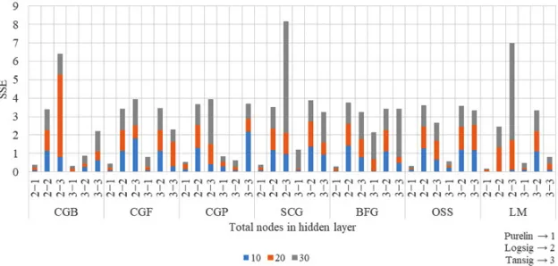
Fig. 5. Effect of Error Sum of Squares on total nodes in hidden layer and activation function on each algorithm The database is split into; training set, validating
set and testing set. A training set is adopted for learning to fit the parameters and is specifically applied to alter the varying weights and errors of the network in each iteration2, 11. Validation set tunes
the four parameters produced as a function to predict the size of the Ag-NPs along with the actual size of the nanoparticle obtained.
MeThODOLOGy
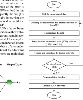
An appropriate ANN model requires a learning algorithm, transfer function, suitable number of hidden layers and neurons. The framework to build and elect the appropriate ANN model for the chosen application is shown in Fig. 2. The most common learning in ANN is the BP technique which uses a supervised learning. A supervised learning paradigm compares the output response to the target response to calculate the learning error. This learning error is used to adjust the network parameters to enhance the performance of the network5. In this paper, the designed network has four input parameters and one output parameter. Thus, the ANN is constructed with 4 neurons in the input layer and the output layer with 1 neuron. The number of neurons in the hidden layer and the transfer function is tested against to find the best suitable architecture for the application. The final evaluation of each network operation is done using Mean Square Error (MSE), Mean Absolute Error (MAE), Error Sum of Squares (SSE) and Regression (R).
The values of these indices can be calculated using the following equations,
...(1)
...(2) ...(3) where, n is the number of points, Yi is the value predicted from the ANN model and Pi is the actual value2. R, the determination coefficient of linear regression, is a line between the predicted values from the ANN model and the target output. It fits better to the actual data when the R value tends to 112.
ReSULTS AND DISCUSSIONS
All 7 algorithms used are coded in MATLAB with R2012b (8.0.0.783) version. The study is carried out by choosing one input, hidden and an output layer. The architecture of the ANN model is changed by altering the number of neurons in the hidden layer (10, 20, and 30) along with
the transfer functions (purelin, logsig and tansig) in both hidden and output layer. Table II presents the values obtained by various architectures and transfer function arrangements of each algorithm. Normalization of all the input data in accordance with the transfer function is the first step of the calculation before using the neural networks. The last step is the de-normalization of the output data2. For enhanced performance and selecting the optimum architecture for the application, the performance indicators ((1)-(3)) and R between the target response and the output obtained are analyzed.
Other values of the indices comprising MSE, MAE and SSE are recorded in Fig. 3, 4 and 5. The transfer function is applied to both hidden and output layer in the ANN model. Therefore for example, in Fig. 3. (2-1) explains the use of Logsig transfer function in the hidden layer and Purelin transfer function in the output layer. All the other combinations follow the same pattern.
The values of indices are computed using the MATLAB syntax in the code itself. As presented in Table II, the optimum network model for this application for traincgb is when the network has 10 neurons in the hidden layer and logsig; purelin as the activation function in the network. The MSE corresponding to this is 0.003. It can be seen that all the other readings for MSE are bigger than MSE reading for the optimum network found. The R values for this network are 0.9864, 0.9877 and 0.9711. For traincgf the optimum network is found to be 10, logsig; purelin with MSE value as 0.027 and R value as 0.9880, 0.9981 and 0.9784 whereas traincgp gives the optimal results when the network architecture and parameters are set to 10, tansig; logsig where MSE value is seen to be 0.0026 and R values as 0.9924, 0.9824 and 0.9634. The trainscg algorithm gives better results with 10, tansig; purelin as its architecture and activation function. The MSE value for the same is found to be 0.0028. 0.9882, 0.9885 and 0.9932 are the R values. However, it is seen that MSE values for trainbfg algorithm, 0.0018, is same for when the network is 10, logsig; purelin and 10, tansig; purelin. In this case, the optimal network is chosen by comparing the R values and the best validation giving the most favorable architecture in
trainbfg as 10, logsig; purelin with best validation
0.9663, 0.9917 being the R values. In trainoss the finest value of MSE is 0.0027 whereas R is 0.9838, 0.9881, 0.9745 with the network parameters as 20, logsig; purelin. Finally for trainlm, MSE value is recorded as 0.00007 with R values nearest to 1; 0.9977, 0.9968 and 0.9959 when the network had 10 number of neurons in the hidden layer and logsig; purelin as the activation function.
Effect of each of the seven algorithms on the output response by varying the architecture of the ANN model and the transfer function in hidden and output layer is shown in Fig. 3, 4 and 5. ANN models that are simulated using numerous training functions are altered in accordance with the number of neurons in their hidden layer. MSE of all the responses recorded is illustrated in Fig. 3. MSE is an important criterion for measuring the overall performance of a designed ANN model. Fig. 4 illustrates a graph between the MAE and total number of nodes in the hidden layer and activation function for all the 7 algorithms used to design the various ANN models. The absolute value of the difference between the target value provided to the ANN model to train and the actual value obtained is the absolute error. Fig. 5 illustrates a graph between error sum of squares, which computes the total deviation of the obtained values from the fitting line or the regression line, and total number of nodes in the hidden layer and activation function. Smaller the value of SSE, better will be the regression line. It is sometimes
CONCLUSION
In this research, the size of the Ag-NPs is determined using ANN modeling from different combinations of architectures and transfer functions by means of a feed-forward neural network model which renders the effect of volume
of C. longa extraction, stirring time, temperature,
and volume of AgNO3 on the nanocomposites behavior. The ANN model is simulated, trained and tested with the learning algorithms like Quasi-Newton, Conjugate Gradient and Levenberg-Maquardt using the dataset. In the projected work it is evident that Levenberg-Maquardt is the best suited algorithm when considering engine data set type for the particular application. It converges in lesser epochs and indeed takes shorter time period than all the other training algorithms. Some
suitable architectures gave worthy performances within the same algorithms as their R value is observed nearest to 1. The experiment shows that ANN is an effectual tool in pondering subjects related to nanoengineering as the size of the silver nanoparticle is predicted in the absence of the costly and time-consuming tests.
ACKNOWLeDGeMeNT
The authors would like to acknowledge & thank Dr. V. Ganapathy, Professor in SRM Institute of Science & Technology, Kattankulathur for his immense help in this work.
ReFeReNCeS
1. Ibrahim Khan, Khalid Saeed, Idree S khan, “Nanoparticles: Properties, applications and toxicities”, Arabian Journal of Chemistry (2017), Available: http://dx.doi.org/ 10.1016/j. arabjc.2017.05.011.
2. P. Shabanzadeh, N. Senu, K. Shameli, F. Ismail, “Application of Artificial Neural Network (ANN) for Prediction Diameter of Silver Nanoparticles Biosynthesized in Curcuma Longa Extract”, Digest Journal of Nanomaterials and Biostructures, 8(3), pp. 1133 – 1144 (2013). 3. Steven J. Oldenburg, “Silver Nanoparticles:
Properties and Applications”, Sigma-Aldrich, Available: https://www.sigmaaldrich.com/ technical-documents/articles/materials-science/ nanomaterials/silver-nanoparticles.html. Accessed: (2018).
4. G M Sacha, P Varona, “Artificial intelligence in nanotechnology”, Nanotechnology,24: no. 452002 (2013).
5. Mohammad Hemmat Esfea, Masoud Afranda, Somchai Wongwisesb, Ali Naderic, Amin Asadid, Sara Rostamia, Mohammad Akbaria, “Applications of feedforward multilayer perceptron artiûcial neural networks and empirical correlation for prediction of thermal conductivity of Mg(OH)2–EG using experimental data”, International Communications in Heat and Mass Transfer, 67: pp. 46–50 (2015).
6. Howard Demuth, Mark Beale, Martin Hagan, “Neural Network Toolbox™ 6 User’s Guide”, COPYRIGHT 1992–2008. Available: http:// citeseerx.ist.psu.edu/viewdoc/ download?doi= 10.1.1.144.5444&rep=rep1&type=pdf.
Brain CT Images”, IOSR Journal of Computer Engineering (IOSR-JCE), 16(1): pp. 31-35 (2014).
8. A. D. Dongare, R. R. Kharde, Amit D. Kachare, “Introduction to Artificial Neural Network”, International Journal of Engineering and Innovative Technology (IJEIT), 2(1): pp. 189-194 (2012).
9. Jonathan Richard Shewchuk, “An Introduction to the Conjugate Gradient Method Without the Agonizing Pain”, edition 1 , Carnegie Mellon University, Pittsburgh, August 1994. Available: https://www.cs.cmu.edu/~quake-papers/ painless-conjugate-gradient.pdf. Accessed: March 17, 2018.
10. Islam El-Nabarawy, Ashraf M. Abdelbar, Donald C. Wunsch Ii, “Levenberg-Marquardt and Conjugate Gradient Methods Applied to a High-Order Neural Network”, The 2013 International Joint Conference on Neural Networks (IJCNN), Dallas, TX, pp. 1-7 (2013).
11. Jason Brownlee, ”What is the Difference Between Test and Validation Datasets? - Machine Learning Mastery”, [Online]. Available: https:// machinelearningmastery.com/difference-test-validation-datasets/. Accessed: March 17 (2018). 12. Shyam S Sablani, Oon-Doo Baik, Michele