www.nat-hazards-earth-syst-sci.net/15/2037/2015/ doi:10.5194/nhess-15-2037-2015
© Author(s) 2015. CC Attribution 3.0 License.
Multi-variable bias correction: application of forest fire risk
in present and future climate in Sweden
W. Yang, M. Gardelin, J. Olsson, and T. Bosshard
Swedish Meteorological and Hydrological Institute, Norrköping, Sweden Correspondence to: W. Yang ([email protected])
Received: 14 November 2014 – Published in Nat. Hazards Earth Syst. Sci. Discuss.: 30 January 2015 Revised: 29 June 2015 – Accepted: 10 July 2015 – Published: 11 September 2015
Abstract. As the risk of a forest fire is largely influenced by weather, evaluating its tendency under a changing climate be-comes important for management and decision making. Cur-rently, biases in climate models make it difficult to realisti-cally estimate the future climate and consequent impact on fire risk. A distribution-based scaling (DBS) approach was developed as a post-processing tool that intends to correct systematic biases in climate modelling outputs. In this study, we used two projections, one driven by historical reanalysis (ERA40) and one from a global climate model (ECHAM5) for future projection, both having been dynamically down-scaled by a regional climate model (RCA3). The effects of the post-processing tool on relative humidity and wind speed were studied in addition to the primary variables precipita-tion and temperature. Finally, the Canadian Fire Weather In-dex system was used to evaluate the influence of changing meteorological conditions on the moisture content in fuel layers and the fire-spread risk. The forest fire risk results using DBS are proven to better reflect risk using observa-tions than that using raw climate outputs. For future periods, southern Sweden is likely to have a higher fire risk than to-day, whereas northern Sweden will have a lower risk of forest fire.
1 Introduction
A forest fire is an uncontrolled fire event. It can exert a destructive influence on ecosystems, affecting climate and weather (Flannigan, 2009). On the other hand, it also has beneficial effects on wilderness areas where some species
de-pend on prescribed fire for growth and reproduction (Brock-way and Lewis, 1997) and on fire hazard reduction (Fernan-des and Botelho, 2003).
Forest fire activity is strongly affected by two factors: weather conditions and availability of fuels. The weather conditions directly and indirectly affect fire behaviour dur-ing both ignition and burndur-ing by influencdur-ing the fuel con-ditions, especially through the moisture content in the up-permost dead fuel (Fosberg and Deeming, 1971). Over the past century, global warming caused by an anthropogenic in-crease in greenhouse gases has shown its impact on present climate (IPCC, 2007). This is likely to have even more of an impact if these gases continue to increase with human activi-ties. The changing climate will thus likely accelerate the wa-ter cycle on a global scale, subsequently intensify the uneven distribution of precipitation, and cause more extreme weather conditions locally (IPCC, 2013). Studying the changes in fuel conditions caused by changing climate is hence impor-tant for decision making, both for public authorities and in forest management.
lightning ignition (Granström 1993). Extreme weather condi-tions, such as the conditions prior to and during the Sala fire (i.e. extremely low relative humidity, strong wind speed and extreme high temperature), are also one of the causes that make fuels conductive to ignition and spread (Fendell and Wolff, 2001; Ryan, 2002). Dendrochronological fire studies have indicated a large temporal and spatial variability in fire activity in Sweden during the last 500 years (Niklasson and Granström, 2000; Drobyshev et al., 2014). A recent study by Drobyshev et al. (2014) reveals that a geographical division between one northern and one southern region with different characteristic fire activity could be found around 60◦N.
In climate change studies, global climate models (GCMs) and regional climate models (RCMs) are widely used tools to simulate climate at different scales. RCMs in general out-perform GCMs in many aspects due to (1) a better represen-tation of geographical features such as orography, thanks to finer spatial resolution (typically at 25–50 km), and (2) a bet-ter description of physical processes by means of, e.g. sub-grid-scale parameterisation and more detailed land surface schemes (Giorgi and Marinucci, 1996; Samuelsson et al., 2010). However, the mismatch between RCM-simulated and observed climatological conditions still cannot be neglected. A study conducted by the Swedish Commission on Climate and Vulnerability (SOU, 2007) demonstrated the limitations of using raw data from a climate model for forest fire danger estimation, as historically simulated fire danger levels were consistently lower compared to risk levels estimated using meteorological observations. This discrepancy is very likely caused by biases in driving variables from climate model out-puts.
One conventional approach to tackle climate model bias is the delta change method by which an observed data time se-ries is perturbed with a projected climate change (Flannigan et al., 1991; Stocks et al., 1989; Hay et al., 2000). Typically, the changes in long-term climatology on a monthly or sea-sonal basis are superimposed on the observation records over the entire frequency distribution, i.e. for both extreme and normal events. This approach is easy to implement and keeps exactly the same change in climatological mean in meteoro-logical variables as that in climate projection, but with two limitations. The first limitation is that only average change in monthly variables is incorporated. The variance in future climate comes either from observed data or from perturbed data, but it does not directly come from climate projection. The second limitation is that changes in regional climate (i.e. one grid cell) are assumed to be the same for all loca-tions in the same region, which is very unlikely to be true. Another widely used approach in forest fire risk studies is built on the statistical relationship of weather conditions on the point scale (i.e. single station) and at its corresponding climate model grid cell (Mearns et al., 1995; Logan et al., 2004). The approach has been applied in a number of case studies (Bergeron and Flannigan, 1995; Wotton et al., 2003). By this approach, various correction processes were designed
for different variables: (1) precipitation frequency and hu-midity magnitude are corrected using the statistical relation-ship identified under present climate; (2) noon temperature is simply estimated as modelled maximum daily temperature minus 2.0◦C and (3) wind speed comes directly from model output and remains uncorrected. This approach makes model output more realistic for use in fire risk studies; however, it merely treats a small part of the bias in variables in a simple way, that is, the frequency of rainy days is corrected but not precipitation magnitude; humidity variables are corrected in terms of long-term mean but without consideration of vari-ance; no treatment is carried out for bias in modelled maxi-mum daily temperature and wind speed.
Recently, the quantile-mapping approach has been de-veloped to correct bias in climate model outputs. The ap-proach mainly focuses on correcting the biases in precipita-tion (and/or temperature) from RCMs to better reflect obser-vations via mapping either parametric or non-parametric cu-mulative distribution functions (CDFs) to observed and pro-jected climate variables (Piani et al., 2010; Themeßl et al., 2011; Yang et al., 2010). A few studies have focused on cor-recting RCM bias in other hydrologically relevant meteoro-logical variables, e.g. relative humidity, wind speed and solar radiation (Wilcke et al., 2013).
This study presents work regarding the forest fire risk in Sweden under changing climate. The forest fire model, ob-servations and climate data are introduced in Sect. 2. The systematic bias originated from RCMs is removed by one of the quantile-mapping approaches, the distribution-based scaling (DBS), which is extended to support bias correction of wind speed and relative humidity (see Sect. 3). Follow-ing the experimental set-up in Sect. 4, the newly developed approach was calibrated and validated, and then further ap-plied to the impact study. Ultimately, an impact study was carried out via two RCM simulations, one reanalysis-driven historical run for method development and validation under present climate and one GCM-driven future projection for estimating the climate change impact. Their corresponding results are discussed in Sect. 5. At the end of the paper, some conclusions and remarks on future development are given in Sect. 6. A summary of acronyms and variables are listed in Table A1a and b.
2 Fire risk model and data
2.1 Fire Weather Index system (FWI)
The details of the application of the FWI can be found in Van Wagner (1987) and Dowdy et al. (2009). Here, only the key features of each component are summarised. The FWI system tracks daily moisture content variations in three stratified fuel layers in forests, coded as primary indices: the Fine Fuel Moisture Code (FFMC), the Duff Moisture Code (DMC) and the Drought Code (DC). For every index, two phases are considered: the rainfall phase and the dry-ing phase. They are determined by a threshold value given as an empirical value in the FWI literature for the purpose of each index. Any rainfall below the threshold value is to be ignored in individual layers. As the three layers differ in fuel type and in their connections to the weather conditions in the proximity, they play different roles in potential fire be-haviour. What they have in common are the influencing fac-tors. They are present as moisture content in the fuel, drying rate and weather states of being dry or wet (i.e. rainy or non-rainy days).
2.1.1 Primary indices: FFMC, DMC and DC
The uppermost surface layer, described by the FFMC, re-sponds rapidly to the short-term changes in weather condi-tions that are described by precipitation, P (mm), tempera-ture,T (◦C), relative humidity, RH (%) and wind speed,W (m s−1). It is the most important layer in the FWI and other fire risk models when assessing fire risk.
The middle layer is a loosely compacted organic layer on the forest floor. The DMC was designed to reflect its average moisture content. It gives an indication of the slow-drying forest fuel consumed in burning. This layer is influenced by all input variables except wind speed. Again, the moisture content, mc (%), is an indicator to reflect the moisture condi-tion in the fuel.
In contrast to the computation in the FFMC layer, the dry-ing rate,k(log10% day−1), in the DMC layer is calculated as proportional not only to temperature and the deficit in rela-tive humidity but also to the day length varying with season,
Le(h).
The bottom layer is a very slow-drying compact organic fuel in the deeper soil layers. Its corresponding code, DC, re-flects the influence of long-term drying on the fuels (Turner, 1972). It is used to detect extremely long dry conditions in lower layers of deep duff, which may result in persistent smouldering.
This layer does not have direct contact with the atmo-sphere. It only absorbs moisture through rainfall and dries out through the evapotranspiration process. Therefore, its fi-nal code computed from moisture equivalent is a function of the previous code value and potential evapotranspiration,V (mm day−1).
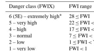
Table 1. Range of FWI (Fire Weather Index) for fire danger classes in Sweden.
Danger class (FWIX) FWI range
6 (5E) – extremely high∗ 28≤FWI
5 – very high 22≤FWI<28
4 – high 17≤FWI<22
3 – normal 7≤FWI<17
2 – low 1≤FWI<7
1 – very low FWI<1
∗in operational use; danger class 6.
2.1.2 Integral indices: Build-Up Index, Initial Spread Index and Fire Weather Index
The Build-Up Index (BUI) and the Initial Spread Index (ISI) are two intermediate sub-indices computed based on the aforementioned primary moisture indices. They were de-signed to describe the fire behaviours, the available fuel and the rate of fire spread for combustion. BUI is built up by the combination of the DMC and the DC. It indicates all fuel available for consumption during the burning process. ISI is computed by combining moisture content in the fine fuel and W using a wind function, f (W ), and a fine fuel moisture function,g(FFMC) (Van Wagner, 1987). It is used as an in-dicator for the potential rate of fire spreading.
Ultimately, the Fire Weather Index (FWI) is an integrated function of a function of ISI,h(ISI), and a function of ISI, l(BUI), to represent fire intensity as energy output rate per unit length of fire front.
2.1.3 Application of the FWI system in Sweden
Swe-den. The FWI system is therefore chosen for climate change impact studies.
2.2 Data
2.2.1 Observations
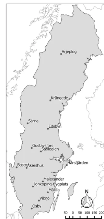
Data were compiled from meteorological stations with ob-served 24 h accumulated precipitation (P-obs) as well as temperature (T-obs), wind speed (W-obs) and relative hu-midity (RH-obs) at 12:00 UTC, covering a reference period from 1966 to 2005. They were extracted from the Swedish network of observation stations (see Fig. 1) with at least 30-year long measurements with less than 20 % missing values in the reference period, to ensure coverage of various cli-mate phenomena. The following requirements were consid-ered: (1) data must be geographically evenly distributed to represent most of the Swedish climatic regions and (2) ob-servations must be of a high quality. It should be emphasised that wind speed is inherently hard to measure in a consistent way over long time periods because the instruments are repo-sitioned, nearby buildings are put up or torn down, forests grow up or get cut, etc. Nevertheless, some findings can be summarised by analysing the observations, which will be de-scribed in Sect. 5.1.1.
2.2.2 RCM simulations
Two climate simulations, denoted as RCA3-ERA40 and RCA3-E5r3-A1B, were used in this study. They were both dynamically downscaled to 25 km resolution by the RCM, the RCA3, but driven by different large-scale forcing data as lateral boundaries. The RCA3 is the third full release of the Rossby Centre regional climate model, developed at the Swedish Meteorological and Hydrological Institute (SMHI) (Samuelsson et al., 2010). For many near-surface variables, the RCA3 represents the European climate well when com-pared to other RCMs (Hagemann et al., 2004).
The RCA3-ERA40 simulation uses the ERA40 reanalysis data as its boundary condition and covers the period from 1961 to 2000. It is assumed to represent the reality as repre-sented by local observations and was therefore used to verify the methodology in this paper. The RCA3-E5r3-A1B tran-sient projection from 1961–2100 is based on the ECHAM5 GCM (Roeckner et al., 2006), forced with the IPCC emis-sions scenario A1B, an intermediate scenario with respect to the magnitude of future global warming (Nakicénovi´c et al., 2000). In this experiment, the RCA3-E5r3-A1B projection was first evaluated for past climate and then used for future impact assessment. Within the ensemble of 16 climate pro-jection studies by Kjellström et al. (2011), RCA3-E5r3-A1B represents projections in the small-to-medium range with re-spect to the expected future increase of bothP andT.
The same variables as those collected at observation sta-tions were extracted for the following experiment. They are
Figure 1. Map showing the locations of the observation stations.
grid-averaged daily precipitation (P-raw), 2 m temperature (T-raw), 2 m relative humidity (RH-raw) and 10 m wind speed (W-raw). Time series from the RCA3 grid cell cov-ering each of the stations were used.
3 RCM bias correction for fire risk modelling
The DBS method is a parametric quantile-mapping ap-proach. It aims to correct systematic bias in GCM/RCM out-puts while preserving the temporal variability in meteorolog-ical variables resulting from climate projections over time. In DBS, as opposed to common non-parametric quantile-mapping approaches, meteorological variables are fitted to appropriate parametric distributions that allow for generation of values outside the range of the reference period and thus simulation of previously unobserved conditions in future cli-mate periods.
The general form of the DBS approach is
xSimCorr=FObs−1hFSim
xSimOrg, γSim, ϕSim
, γObs, ϕObs
i
where γ andφ are distribution parameters estimated from the climate model (subscript Sim) and from the observa-tions (subscript Obs) by the maximum likelihood estima-tor (MLE), the method of moments, iterative or other ap-proximate methods;xSimOrgis the original output of variablex simulated by a climate model andxSimCorris the result after cor-rection.FSimandFObs−1 stand for the cumulative distribution function (CDF) and its inverse of a suitable parametric dis-tribution for each variable of interest.
The distribution parameters of precipitation are estimated for every season, whereas the distribution parameters of other variables are estimated using a 31-day moving window for every Julian day, and Fourier series are used to describe the distribution parameters over the year in a smooth way:
γ t∗=a0
2 + K X
k=1
[akcos(kwt·)+bksin(kwt·)] (2)
φ t∗=c0
2 + K X
k=1
[ckcos(kwt·)+dksin(kwt·)], (3)
wherea0,ak,bk,c0,ck anddk are the Fourier coefficients, t∗is the day of the year;wequals 2π/n, wherenis the time units per cycle (in our case 365 days) and kstands for the nth harmonic. Theoretically, (t∗/2+1) harmonics are able to represent a complete cycle perfectly, with the drawback of a potential overfitting of the data. Five harmonics have been found to be sufficient in Yang et al. (2010).
3.1 DBS forP andT: an overview
A detailed description of the DBS for P andT correction can be found in a previous study by Yang et al. (2010). In the following, only a summary is given.
To tackle the common RCM bias in terms of the overes-timated frequency of rainy days with small rainfall amount (i.e. wet frequency bias, “drizzle effect”) a cut-off value is identified as a threshold to correct the frequency of rainy days
(P >0.1 mm) in climate projections. Any drizzle, generated
by the RCM model, with intensity smaller than the threshold is removed, and the day with the drizzle is treated as a dry day. Dry frequency bias, i.e. the tendency of RCMs to under-estimate wet-day frequency, is rather uncommon in Europe but may occur, e.g. during summer in south-eastern Europe and in the Alps (Hagemann et al., 2004; Jacob et al., 2007). In the current DBS method, such wet-day deficit is handled by adding a small rainfall amount at the end of wet spells, starting with the longest ones, until the correct frequency is obtained. In-depth analysis and research work are progress-ing.
After the precipitation frequency bias has been corrected, the remaining modelled precipitation is then transformed to match the distribution of observed precipitation. The full time series is divided into two partitions separated by the 95th percentile identified from sorted observation records
and model simulation. This approach intends to capture the main properties of normal low- to medium-intensity pre-cipitation as well as the high-intensity extremes. A double-gamma distribution, instead of a conventional double-gamma dis-tribution, is accordingly implemented. Two sets of parame-ters –α,β (normal precipitation) andα95,β95(extremes) – are estimated by the maximum likelihood estimator (MLE) from observations and from the RCM output in the refer-ence period. The fitted scaling parameters are then applied to correct the RCM outputs for the entire projection pe-riod by Eq. (1). For impact studies in Europe, four seasons are normally used. They are winter (December–February), spring (March–May), summer (June–August) and autumn (September–November).
Daily temperature values are described using a Gaussian distribution. For every Julian day, the distribution parame-ters,µT andσT, are estimated from observations and RCM data. Considering the dependency between P and T, the statistics of temperature are calculated separately for wet days (i.e. rainy days) and dry days (i.e. non-rainy days). 3.2 DBS for RH andW: method development
The approach for correcting RH andW is similar to that for dailyP andT. The factors used to scale RH andWwere de-fined conditioned on the location of the station and the sea-son of interest. For wind speed scaling, the precipitation state (i.e. wet or dry) is considered as an influencing factor.
Relative humidity is different than other variables in that its value is restricted to the interval of [0, 1]. To cope with this property, the commonly used Beta distribution (Yao, 1974) is chosen, the density distribution of which is
f (x)=
0(p+q)
0(p)0(q)
xp−1(1−x)q−1, (4)
wherepandqare the two parameters of the distribution and 0is the gamma function. By different combinations ofpand q, a wide range of distribution shapes maybe represented. The distribution parameters can be fitted by the method of moments using the equations below:
µ= p
p+q (5)
σ2= pq
(p+q)2(p+q+1), (6)
whereµandσare the statistical mean and standard deviation of the data to be fitted.
the Weibull distribution (Pavia and O’Brien, 1986; Seguro and Lambert, 2000). Its density distribution is given as
f (x)=
κ
λ x λ
exp
−
x
λ κ−1
κ, λ, x0, (7)
where the two parametersκandλare shape and scale param-eters, respectively. The shape parameter,κ, describes numer-ous shapes with different magnitudes of positive skewness, while the scale parameter,λ, controls the stretch of the dis-tribution.
The Weibull distribution has several special forms when setting the shape parameter κ to different values. For in-stance, the Weibull distribution is identical to the gamma distribution when κ equals 1, and it is very similar to the Gaussian distribution whenκequals 3.6. It can also be trans-formed to be an extreme value distribution (EVD) with lo-cation parameter µ=log(κ) and scale parameterσ=λ−1. Because of its particular properties, it can also be used to solve other distributions after transformation. The distribu-tion parameters of the Weibull distribudistribu-tion are convendistribu-tionally estimated using MLE. As its density function is analytically integrable, as expressed in Eq. (8), it is straight-forward to calculate the probability and solve the inverse function:
F (x)=1−exph−x
λ κi
κ, λ, x0. (8)
4 Experimental set-up and evaluation
RCM-simulated P-raw, T-raw, RH-raw and W-raw at 12:00 UTC were bias-corrected using observations from me-teorological stations (see Sect. 3). Along with original out-puts from RCMs and observed variables, the corrected vari-ables were used to drive the FWI system for assessing for-est fire danger. The internal variables (FFMC, DMC, DC) as well as the integrated indices BUI, ISI, the final index (FWI), and the fire danger classes (FWIX) were all used for evaluat-ing the influence of the DBS approach.
To validate the approach, 1966–1985 (20 years) was used as the calibration period for both simulations; 1986–2000 (15 years) was used as the validation period for the RCA3-ERA40 simulation (as the reanalysis data i.e. RCA3-ERA40 ends by 2000), and 1986–2005 (20 years) was used for the RCA3-E5r3-A1B simulation. Basic statistics such as the climato-logical mean (Avg) and the standard deviation (SD1) were calculated in both the calibration and validation periods. For P, the mean value of accumulated seasonal precipita-tion (Acc) is used to present its long-term mean. Because of the discrete-continuous property of precipitation and wind speed, an additional statistic, the frequencies of rainy and windy days are computed to study how the model captures their properties. In the following, they are denoted as Freq-P (i.e. occurrence of days with rainfall amount larger than 0.1 mm) and Freq-Ws (i.e. occurrence of days with wind speed above 0 m s−1). Moreover, a standard distance (SD2)
was included to investigate the spatial variations of every variable. It is computed as the standard deviation of the mean values of all stations. A larger value indicates a higher vari-ability in space, and vice versa.
Apart from that, how well climate models can capture the observed probability distribution of individual variables was also studied using a PDF skill score (SS) (Perkins et al., 2007). The SS is a quantitative assessment of goodness-of-fit in terms of probability distribution to evaluate the consis-tency between two data sets. The results reflect the agree-ment, with a perfect agreement resulting in an SS of 1.0 and a poor agreement in an SS close to 0. In this work, the SS is calculated from observation, raw and corrected RCM out-puts. Its formula is expressed as in Eqs. (9a) and (9b), where m is the number of bins used to calculate the PDF for a given variable per station,Zraw(andZcorrected) is the probability in a given bin from model simulation before and after bias cor-rection, respectively, andZObs is the probability in a given bin from the observed data.
SSraw= m X
1
min(Zraw, ZObs) (9a)
SScorrected= m X
1
min(Zcorrected, ZObs) (9b)
All these statistics were calculated from the climate projec-tions’ output before and after bias correction, and observa-tions. For P, RH and W, their relative differences in Avg were used for bias evaluation, whilst forT, the differences in Avg were used. In terms of the two SD (SD1 and SD2), the ratio of their values calculated from model outputs and from the observations was used to identify the differences in describing the variances.
For future climate change (CC) assessment, the scaling parameters obtained from the reference periods (i.e. 1966– 1995) were applied to individual variables for the future pe-riods in climate projections. Subsequently, the corrected vari-ables were used to run the FWI system. The transient future projections were divided into three 30-year time periods – 2011–2040, 2041–2070, 2071–2100 – for analysing the cli-mate change signals and influence of the DBS method on meteorological variables and further on the forest fire danger in the near, intermediate and distant future. The results for the period 2071–2100 are to be presented in this paper.
5 Results and discussion
5.1 Evaluation for present climate 5.1.1 Meteorological variables
Sweden is characterised as a mixture of temperate and conti-nental climate with four distinct seasons. The seasonal tem-perature varies on average from−4◦C in winter (not shown here) to 18.3◦C in summer (see Table 2). Due to its large cov-erage in latitude, the temperature in Sweden varies greatly from north to south, with 12◦C difference in winter temper-ature and 6◦C difference in summer temperature (not shown here).
Precipitation in Sweden occurs throughout the whole year. In general, it often rains less in spring and winter, whereas it rains heavily in summer and autumn with stronger vari-ability. The rainfall frequency in spring is in the same range as that in summer, but approximately 21 % less compared to that in autumn; however, the accumulative precipitation amount in spring is much lower compared to the other two seasons (i.e. 42.8 % compared to summer and 50.6 % com-pared to autumn), which implies drier conditions in spring (see Table 2 and Fig. 2).
In terms of relative humidity, the distribution varies from season to season. On average, the relative humidity in Swe-den appears to be relatively low in spring and summer (i.e. in the range of 55–65 %) and reaches its minimum value in summer. From autumn onward, its value continuously in-creases until its annual maximum in winter (see Table 2, Figs. 2 and 3).
Annual mean wind speed in Sweden varies between 2 and 5 m s−1, with an average of 4 m s−1. In southern Sweden it is generally high because this region is more exposed to west-erly and south-westwest-erly wind. Wind speed closer to the coast features stronger variability than that in the inner region. Wind speed in the inner regions of central Sweden such as Edsbyn is characterised as a general weak annual cycle with the weakest wind in winter (see Fig. 2).
With respect to its spatial distribution (see SD2 in Table 2) precipitation is a localised variable, while the rest of the vari-ables are largely influenced by large-scale effects.
As reanalysis data (i.e. ERA40) are generally assumed to be the closest data set to the real climate, the deviations from observations in the RCA3-ERA40 run are considered to mainly reflect RCA3 model bias. The main findings from a comparison between observed and RCA3-ERA40 simulated climate statistics include the following (see Tables 2 and 3):
– The seasonal precipitation amount is generally overes-timated for all three seasons, whereas variability is in general slightly lower than that of the observations (see SD1 in Table 2). The climate model estimates the fre-quency of wet days with the lowest accuracy for sum-mer, in which almost 100 % bias was found in compar-ison to the observations; the overestimation in autumn
Figure 2. Seasonal variation of the FWI inputs (precipitation, tem-perature, relative humidity and wind speed) presented as 7-day moving average values at the Edsbyn station (see Fig. 1). Compar-ison of observational data and raw output of the climate models from RCA3-ERA40 and RCA3-E5r3-A1B simulations (calibration period 1966–1985).
was 66.7 % and in spring it was 80.8 %. The average SS had a value of 0.60. Again, the summer precipita-tion is the least accurately simulated, with an SS value of approximately 0.56 (see Table 3). Concerning spatial variability, modelled precipitation tends to be more un-evenly distributed than observations in spring and sum-mer, which is in contrast to the situation in autumn. – A cold bias appears during all fire seasons. The largest
bias (−2.3◦C) was found in summer, whereas the low-est bias (−0.9◦C) appeared in autumn. This is also re-flected by the SS being 0.80 for spring, 0.85 for autumn and 0.71 for summer (see Table 3). Similar to precipi-tation, the spatial variability at point stations is under-estimated by the climate model in autumn (−7.7 %), whereas it is overestimated by ∼30 % in spring and summer.
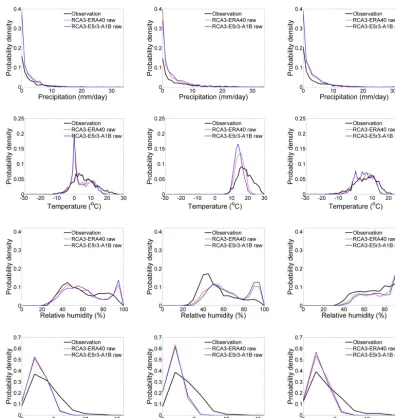
Figure 3. Probability density functions of precipitation, temperature, relative humidity and wind speed at the Edsbyn station (see Fig. 1). Comparison of observational data and raw output of the climate models RCA3-ERA40 and RCA3-E5r3-A1B (calibration period 1966–1985).
in the modelled data for the fire season except for au-tumn (−14.3 %).
– Wind speed and its variance are evidently underesti-mated during all seasons of interest. Its distribution is positively skewed but with a larger proportion of low wind speeds and a smaller proportion of high wind speeds in the simulated data (Fig. 3). In the RCM run, Ws-raw of more than 6 m s−1seldom occurs, which dif-fers from that in the observations, in which speeds up to 15 m s−1 occur. The SS is on average 0.70 (see Ta-ble 3). In contrast to the other variaTa-bles, for modelled wind speed the Std2 is significantly lower (∼ −75 %) than that in the observations. Such a damped spatial
variability is noted in all fire seasons, as shown in Ta-ble 2.
observa-tions in cold condiobserva-tions and changing surroundings affecting wind gauges.
Apart from that, the biases are also likely caused by lim-itations in the climate models’ process descriptions. Biases in precipitation may be linked to an overestimation of cloud fraction in mountainous areas (Willén, 2008), incorrectly solved convective triggering and lack of details in geograph-ical information, which lead to unrealistic precipitation sim-ulation. The cold bias (∼ −2◦C) in summer and in autumn over northern Europe may be partly because of an overes-timation of cloud water by the RCA3, which leads to too much short-wave radiation being reflected and subsequently an underestimation of the incoming short-wave radiation at the surface (Willén, 2008). Additionally, the bias in relative humidity in summer may be due to overestimated cloud wa-ter that subsequently leads to an underestimation of maxi-mum summer temperatures over northern Europe (Samuels-son et al., 2010). In terms of wind speed, a general bias is noted when comparing model output to long-term climato-logical means. This can be attributed to the parameterisation utilised in unresolved orography, and uncaptured small-scale features, for instance, the influence of hills, lakes, valleys, etc. Furthermore, the incorrect seasonal wind speed varia-tion generated by the climate model implies that the RCA3 model captures large-scale forcing well, but no other influ-encing processes such as seasonal variations and atmospheric stability over land and water that largely influence the wind speed (Achberger et al., 2006). For inland stations, such as Edsbyn, the seasonal variation in stability over the land is smaller than that over the sea, which reduces the seasonal wind speed variation compared to stations close to the sea (Achberger et al., 2006). However, it seems that Edsbyn was modelled as a coastal location where winter wind speed is enhanced because of less stably stratified atmosphere over water and the stronger pressure gradient in winter.
Bias in GCM-forced RCM runs reflects the integral influ-ence of GCM and RCM. In comparison of the two RCA3 simulations, the reanalysis-forced run (i.e. RCA3-ERA40) is found to outperform the GCM-forced run (i.e. RCA3-E5r3-A1B), however, the difference is overall small and their annual cycles are very similar (see Fig. 2). As shown by the statistics in Table 2 and frequency distribution in Fig. 3, the RCA3-E5r3-A1B generally performs similarly or worse in terms of the statistical mean and variability. The largest differences appear for precipitation simulation for which RCA3-E5r3-A1B generated up to 105 % higher wet-day percentage and 118 % more accumulated precipita-tion than present in the observaprecipita-tions in summer. In terms of precipitation frequency distribution, RCA3-ERA40 tends to generate a slightly higher number of days with small rainfall amount and fewer days with extreme amounts. Temperature is another variable with visible differences between the two simulations. Again, the largest differences appear in summer in which RCA3-E5r3-A1B is inclined to be slightly colder and with less variability than RCA3-ERA40. The
distribu-Figure 4. Seasonal variation of the FWI inputs (precipitation, tem-perature, relative humidity and wind speed) presented as 7-day moving average values at the Edsbyn station (see Fig. 1). Compar-ison of observational data, raw output of the climate models from RCA3-E5r3-A1B simulation and its corresponding corrected output (validation period 1986–2005).
tions of relative humidity and wind speed generated from two simulations are in general almost identical.
Though the two climate projections are driven by different forcing, many of their characteristics are highly consistent, implying that the majority of the biases are likely to originate from the RCM. The alternative conclusion would be that the ERA40 is as bad as the GCM in simulating the statistics of these four variables.
As the climate projection forced by GCM is the basis for assessing future impact, we will mainly focus on evaluating the results from RCA3-E5r3-A1B in the following.
5.1.2 Effect of the DBS approach
Figures 4 and 5 illustrate how the DBS method improves the FWI input variables. In the calibration period (not shown here) the bias correction effectively removed the majority of biases in all of the variables, which is expected as the bias-correction parameters have been calibrated on the same set of data. In the following we will focus the analysis on the validation period to illustrate the effect of DBS.
Table 3. PDF skill scores (SS) of raw data from RCA3-ERA40 and RCA3-E5r3-A1B (1966–1985), averaged over 14 Swedish stations.
Precipitation Temperature Relative humidity Wind speed
Mean Min Max Mean Min Max Mean Min Max Mean Min Max
MAM
RCA3-ERA40 0.64 0.59 0.69 0.80 0.74 0.86 0.83 0.76 0.87 0.75 0.65 0.84
RCA3-E5r3-A1B 0.65 0.60 0.70 0.80 0.75 0.85 0.81 0.76 0.86 0.69 0.57 0.76
JJ
A RCA3-ERA40 0.56 0.48 0.60 0.71 0.67 0.76 0.72 0.63 0.78 0.70 0.55 0.83
RCA3-E5r3-A1B 0.54 0.45 0.60 0.59 0.54 0.63 0.67 0.60 0.72 0.66 0.52 0.76
SON
RCA3-ERA40 0.62 0.58 0.58 0.85 0.89 0.81 0.78 0.74 0.89 0.76 0.62 0.86
RCA3-E5r3-A1B 0.61 0.68 0.65 0.82 0.79 0.79 0.74 0.69 0.84 0.68 0.58 0.83
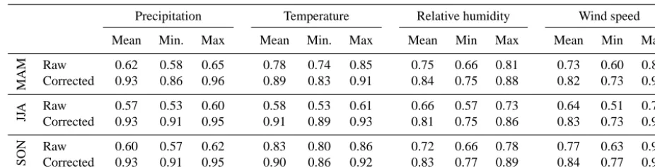
Table 4. PDF skill scores (SS) of data from raw and corrected RCA3-E5r3-A1B (1986–2005), averaged over 14 Swedish stations.
Precipitation Temperature Relative humidity Wind speed
Mean Min. Max Mean Min. Max Mean Min Max Mean Min Max
MAM
Raw 0.62 0.58 0.65 0.78 0.74 0.85 0.75 0.66 0.81 0.73 0.60 0.88
Corrected 0.93 0.86 0.96 0.89 0.83 0.91 0.84 0.75 0.88 0.82 0.73 0.93
JJ
A Raw 0.57 0.53 0.60 0.58 0.53 0.61 0.66 0.57 0.73 0.64 0.51 0.77
Corrected 0.93 0.91 0.95 0.91 0.89 0.93 0.81 0.75 0.86 0.83 0.73 0.94
SON
Raw 0.60 0.57 0.62 0.83 0.80 0.86 0.72 0.66 0.78 0.77 0.63 0.92
Corrected 0.93 0.91 0.95 0.90 0.86 0.92 0.83 0.77 0.89 0.84 0.77 0.92
main, as shown by Fig. 4. The improvement in tempera-ture is noticeable in terms of both the full distribution and the annual cycle. The major improvement occurs for sum-mer and spring where the cold bias appears in modelled data. The corrected T is statistically equivalent to that from the observations in terms of climatological mean and standard deviation of temperature conditioned on dry and wet days. As with temperature, the corrected relative humidity shows a better annual distribution. The overestimation of relative humidity is largely reduced, but some bias still remains at the tail of the distribution. Wind speed gets substantially im-proved in terms of both magnitude and annual distribution. The overestimated number of days with small wind speeds is reduced, and the probability of higher wind speed is largely improved, but the DBS-corrected data tend to overestimate the wind speeds over 6 m s−1. Taking a closer look at the PDF of meteorological variables from different data sources by comparison of Figs. 3 and 5, we find that the effect of the DBS largely depends on the performance of raw climate projections. Whether the climate model is capable of reflect-ing the changes between the calibration and validation pe-riod is very significant. In observation time series, the local climate at the Edsbyn station is found to be warmer (except for summer) and wetter (except for autumn) in the valida-tion period than that in the calibravalida-tion period. The largest rise in temperature appears in winter (i.e. 2.2◦C), followed by a large rise in spring (i.e. 0.9◦C) and a moderate rise in autumn (i.e. 0.4◦C). In summer, the temperature is found to drop by 0.7◦C. For precipitation the seasonal precipitation is found to be wetter in spring (i.e. 4.3 %) and summer (i.e. 13.3 %), but drier in winter by 14.0 % and in autumn by 11.7 % (not shown here). In the climate model’s output (i.e. the RCA3-E5r3-A1B) for the same period a similar trend for tempera-ture is found but with smaller magnitude; however a different trend for precipitation is found. The climate model simulates generally wetter conditions in the validation period over the whole year with a rise of more than 10 % per season except for autumn (i.e. 6.6 %). The increment in spring and sum-mer may even reach 15.0 and 13.6 %, that is, the climate model does not correctly capture the trend in variables and also largely overestimates their changing rate. As a result,
unstable statistics in raw climate projections make it difficult to obtain a correction as good as in the calibration period, which subsequently leads to an imperfect match in fire risk index, e.g. the DC in Fig. 6.
Apart from computed statistics, the distribution correc-tions are also reflected by the SS. The SS in Table 4 show general improvement in all variables, i.e. the SS are on aver-age∼0.93 for precipitation,∼0.90 for temperature,∼0.83 for relative humidity and 0.83 for wind speed, though the sea-sons differ. The largest improvements appear in the summer season in which the major biases tend to occur in the raw cli-mate projections. Similar improvement was found when the correction was applied to the RCA3-ERA40 run (not shown here).
5.1.3 Forest fire risk indices
The major forest fire risk indices – FFMC, DMC, DC, BUI, ISI and FWI – are plotted as long-term average annual cycles over the calibration (1966–1985) and the validation (1986– 2005) periods in Figs. 6 and 7.
a) 1966-1985 b) 1986-2005
Figure 6. Seasonal variation of FFMC, DMC and DC index at the Edsbyn station (see Fig. 1). Comparison of values based on ob-servations (black line), raw output from climate model (blue line),
RCA3-E5r3-A1B, correctedP (precipitation),T (temperature) and
uncorrected RH (relative humidity) andW(wind speed) (green line)
and correctedP (precipitation),T (temperature), RH (relative
hu-midity) and W (wind speed) (red line) for period (a) 1966–1985
(calibration) and (b) 1986–2005 (validation). Note that the DC is
in-fluenced byP (precipitation) andT (temperature) (see blue, green
and black lines).
thus of uttermost importance when climate projections are utilised for forest fire risk assessment.
The DC is an integrating index reflecting the combined ef-fect of precipitation and temperature; it was therefore used to study the correcting impact induced by the DBS on these two variables. As the rainfall cut-off values for all stations are seldom above 2.8 mm (i.e. the threshold values given in the FWI literature, described in Sect. 2.1), the major impact on the DC values is considered to be from the correction of P andT. During the drying phase, the moisture depletion is governed by evapotranspiration, which is proportional to noon temperature and also influenced by the seasonal day-length. During the rainfall phase, any rainfall more than the threshold value is first reduced to an effective rainfall by a linear function and then simply added to the existing mois-ture equivalent. After bias was removed, the corrected noon temperature was in general increased, which led to stronger
a) 1966-1985 b) 1986-2005
Figure 7. Seasonal variation of BUI, ISI and FWI index at the Edsbyn station (see Fig. 1). Comparison of values based on ob-servations (black line), raw output from climate model (blue line),
RCA3-E5r3-A1B, correctedP (precipitation) andT (temperature)
uncorrected (raw) RH (relative humidity) and W (wind speed)
(green line) and correctedP (precipitation),T (temperature), RH
(relative humidity) and W (wind speed) (red line) for period
(a) 1966–1985 (calibration) and (b) 1986–2005 (validation).
evapotranspiration. Additionally, the reduction of precipita-tion amounts (see Figs. 4 and 5) resulted in less moisture equivalent. Ultimately, the fire risk in the slow-acting fuel, described by the DC value, was found to be considerably en-larged in comparison to that which was computed using raw climate output (see Fig. 6) as well as closer to that computed using observations.
phase, the DBS not only removed the small rainfall events but also reduced the portion of medium-size rainfall events via correcting the precipitation distribution (see Figs. 4 and 5). As a result, the overestimated moisture level and conse-quently also the integral value of the DMC were corrected (see red line in Fig. 6). In comparison to the DMC value computed by corrected P and T (i.e. denoted as corrected P T and marked by a green line in Fig. 6), correcting RH andW(red line) leads to additional improvement. Especially in summer and autumn seasons, the maximum improvement reaches as much as 50 %. It is likely because of the removal of drizzle in the precipitation frequency correction that the moisture content in the fuel reduced.
The FFMC reflects the integrated effect of all meteoro-logical input variables. In the drying phase, its drying rate varies with temperature, relative humidity and wind speed. After applying the DBS, the drying rate was increased upon correcting the cold bias inT, the overestimated RH and the underestimated W, as shown in Figs. 4 and 5. Moreover, the computed equilibrium moisture content by drying and by wetting,EdandEw, became smaller (not shown here). In the rainfall phase, only the current moisture content and rain-fall amount matter. As the cut-off values estimated at all sta-tions were all above 0.5 mm (i.e. the threshold values given in the FWI literature, described in Sect. 2.1), any correction of precipitation frequency influenced the final FFMC value. By applying the DBS, many periods of drizzle were removed and the overestimated precipitation amount was corrected. As a result, (1) the wet spells were shortened and the mois-ture content in the fuels had time to dry out; (2) the fire risks described by the FFMC value largely increased (see red line in Fig. 6).
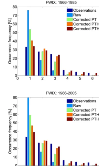
In Fig. 7, the fire behaviour indices, the ISI and the BUI, as well as the final fire risk index, the FWI, were studied. As ISI is a product of wind speed and fine fuel moisture, it is directly influenced when these two are changed. As the W was not perfectly corrected, over- or underestimatedW after bias correction caused larger variation in the ISI index in comparison to that computed using observations. BUI de-pends on the variation in the DMC and the DC values, with more weight given to DMC. Hence, the BUI shows a simi-lar pattern to the DMC index. Ultimately, the final index (the FWI) (Fig. 7) and the fire danger classes (the FWIX) (Fig. 8) used for issuing fire risk warnings (i.e. danger class>=5 in Table 1) were significantly improved.
The fire-risk-related indices generally showed improve-ment when all variables were corrected, compared to only a partial bias correction of precipitation and temperature. This suggests that the bias correction does not destroy the phys-ical consistency between the variables in such a way that it would degrade the validation results when multiple variables are bias-corrected. Apart from that, the improvements imply that the relative humidity and wind speed do play important roles in final fire danger level, and appropriate correction of these two variables adds value to fire risk assessment.
Partic-Figure 8. The occurrence frequency of fire danger classes (i.e. FWIX) at the Edsbyn station (see Fig. 1) calculated from ob-servation, raw climate model output, RCA3-E5r3-A1B, and after correcting meteorological variables.
ularly, the wind speed works as a dominant factor for cases of extremely large forest fire risk (see danger class>=5 in Fig. 8). This finding matches the conclusion drawn from a recent study in Greece (Karali et al., 2014), in which a sensi-tivity test of the FWI indices to the meteorological variables was carried out. It was found that precipitation and wind speed play the most important roles in final indices. Specif-ically, for wind speed, even a moderate wind speed leads to index values over the critical risk thresholds, and a high wind speed results in an extremely high value of the FWI.
cli-Figure 9. Climate change signals inP (precipitation),T (temperature), RH (relative humidity) andW(wind speed) at Edsbyn and Växjö station (see Fig. 1), reflected in RCA3-E5r3-A1B before and after correction during 2071–2100.
mate projection, RCA3-E5r3-A1B, shows obvious underes-timation. No high risk level is reflected at any of the 14 sta-tions (shown in Fig. 11b). After correcting the biases in me-teorological variables, the fire risk in the reference period is significantly increased and it shows a similar spatial distribu-tion pattern to that calculated from observadistribu-tions (see Fig. 11a and c). However, underestimation in the calculated occur-rence of high risk indices (i.e. an average of−6 days per fire
5.2 Future projection (RCA3-E5r3-A1B)
The climate projection was run until the end of 2100 with a transient-mode simulation, which makes it possible to inves-tigate the evolution of climate change in a continuous manner (Kjellström et al., 2006). The historical observations used to obtain the scaling factors cover the period from 1966 to 1995, the longest observation period available for the study area. Topics that will be discussed in this section include whether the DBS alters the climate change signals in input variables as well as the FWI index and how fire risk will evolve in Sweden in the future.
Figure 9 presents the climate change signals in all in-put variables at two stations, Edsbyn in northern Sweden and Växjö in southern Sweden. As projected by RCA3-E5r3-A1B, the local climate in Edsbyn will become wet-ter, warmer, more humid and slightly windier in the future. During fire seasons, a general increase in the precipitation amount is found during the complete future period, partic-ularly during spring in the intermediate and distant future (∼40 % increase). Temperature and relative humidity are also characterised by a general rise during the whole period. The air gets warmer and moister at the beginning of spring in the near future and this tendency is enhanced until 2100. The largest rise appears in spring and the smallest in summer. Compared to the present climate, it is likely to be warmer by 5◦C in 2071–2100 and moister by 15 % in 2071–2100. The change in wind speed is smaller when compared to other variables. It varies mainly within the range of−6 to 6 % in the study periods, with the largest increase in the near future. The maximum increase appears in autumn in every future pe-riod. The local changes in Växjö are projected to be similar to those in Edsbyn, but with stronger seasonal variations dur-ing the fire season. As in Edsbyn, temperature and relative humidity exhibit a consistent future increase. Their rate of increase increases with time until 2100 (i.e. 4◦C warmer and 15 % moister until 2071–2100). The changes of the other two variables fluctuate around zero with a different sign at differ-ent periods of the year. Precipitation decreases during the fire season except in spring, whereas wind speed increases in late summer with a maximum of 10 %.
In general, the corrected data reproduce the climate change signal in the raw climate model output reasonably well. How-ever, in some cases, DBS was found to alter the changes projected by the climate model. It might be caused by non-linearity in RCM biases, that is, the biases caused by an im-perfect model representation of atmospheric physics for the present climate are likely to be altered by the changes in rel-evant climatic variables in the future. For instance, the de-scribed changes in temperature bias can be related to changes in cloud cover and the corresponding response in radiative surface heating, soil moisture feedback and sea level pres-sure (Maraun, 2012), which are not accounted for in the bias-correction approach. As all bias-bias-correction methods, apply-ing DBS is built upon an assumption of stationary bias.
By running the FWI system, the integral impact on the long-term mean future fire risk danger was evaluated (Fig. 10). Because the figures aim to present the average sit-uations for a 30-year period, extreme values cannot be seen. However, their relative changes in FWI compared to those for the present climate are quite consistent though different in magnitude. The differences in CC signal between the raw and DBS-corrected data are partly because of biases in driv-ing variables as described in Sect. 5.1.3. Moreover, as the three primary indices of the FWI (i.e. FFMC, DMC and DC) are computed for drying and wetting phases that are deter-mined by a threshold value for each fuel, any correction of precipitation amount may have an impact on the indices that subsequently influence the final index, FWI, and its CC sig-nals.
Using the corrected data, autumn at the Edsbyn station is found to become more prone to forest fire, followed by spring, and then summer (Fig. 10). It is mainly due to the in-crease of temperature and wind speed. For today’s main fire risk season, summer, the relative change in the FWI value tends to be negative (i.e. approximately−20 %). The moister air, the increased precipitation and relatively stabilised wind speed balance out the effect of the warmer climate. The fire risk in autumn gradually increases with regard to the last 30 years, particularly the beginning of autumn, which is most likely because of relatively drier and warmer air combined with stronger wind speeds. At the Växjö station, the most fire-prone season in future is likely to be summer, where less precipitation, warmer temperatures and higher wind speeds are projected. In the last 30 years, the local climate has be-come even wetter, moister and less windy in spring, which reduces the fire risk level by 15 % compared to the present day. However, the fire risk in summer increases by 20 % as the climate in the distant future becomes drier, warmer and windier.
The relative changes in the number of days with high fire risk (i.e. the FWI>=5) during the fire season are presented in Fig. 11d. Northern Sweden is likely to be a fire-resistant region in the future climate where the number of days with high fire risk is found to be lower than today. In contrast, southern Sweden is projected to become a more fire-prone region where an increased number of days with a high fire risk are found in almost all stations in all three periods. The stations located in central Sweden are projected to face an increased risk of forest fire in the near future, after which the risk decreases until the end of the century. The changes at those stations vary from time to time, which is probably because of local climate factors at different time periods.
6 Conclusions
Figure 10. Climate change signals in the FWI reflected in RCA3-E5r3-A1B for the period of 2071–2100 with respect to the period 1966– 1995 at Edsbyn and Växjö station (see Fig. 1).
a) Observation b) Raw RCA3-E5r3-A1B d) [2071-2100]-[1966-1995]
c) Corrected RCA3-E5r3-A1B Växjö
Edsbyn
Växjö
Edsbyn Edsbyn
Växjö Edsbyn
Växjö
Figure 11. Number of days with high fire risk (FWIX>=5) during the calibration period (1966–1995) presented by (a) observation, (b) raw
RCA3-E5r3-A1B and (c) corrected raw RCA3-E5r3-A1B; and changes of number of days with high fire risk (FWIX>=5) in percentage
during the period of (d) 2071–2100.
climate model outputs show a clear mismatch with the ob-servations in all influencing variables used in fire risk mod-elling: precipitation, temperature, wind speed and relative humidity. This is likely caused by uncertainties in observa-tions as well as improper descripobserva-tions of physical processes and coarse resolutions in the present generation of RCMs.
risk studies. Regarding the simultaneous bias correction of multiple variables, the result showed an improved description of fire-risk-related indices when all variables were corrected, compared to only a partial bias correction of precipitation and temperature. This suggests that the bias correction does not destroy the physical consistency between the variables to such an extent that it degrades the validation results when multiple variables are bias-corrected.
For the present climate, by using bias-corrected meteoro-logical variables, the FWI model generates realistic results that are well in line with those derived from observations. The frequency of extremely high fire risk is significantly bet-ter reproduced when compared to directly using raw climate projection data, though some underestimation remains. Fur-ther development of the DBS method is Fur-therefore required to, e.g. better represent the influencing variables by removing remaining biases, keep consistency amongst meteorological variables in terms of their temporal and spatial covariance and capture the non-stationary climate model biases.
Concerning the future climate, the climate projection used here projects a climate in Sweden that is warmer, wetter and windier than today. Southern Sweden, where it is normally warmer and windier than in other parts of Sweden, is likely to become a more fire-prone region in the future, whereas northern and central Sweden will face a similar or lower fire risk than today. Forest fire activity and its spread is a result of combinations of weather, fuels and topography as well as incident management decisions. Thus, fuel bed structure and fire potential are influencing factors in addition to the changing climate. This kind of studies for Sweden has partly been done previously (Granström et al., 2000; Granström and Schimmel, 1998). With changing climate, there may be a northward displacement of the broad vegetation belts with an increasing component of broad-leaved tree species at the ex-pense of spruce (Koca et al., 2006). Fuel beds in the north may then shift from moss to leaf litter, with unknown ef-fects on ignition potential and fire behaviour. Apart from re-ducing human-caused ignition, experience concerning rescue tactics suppression methods needs to be collated. An ongo-ing project will develop a national preparedness strategy for forest fires with consideration of changing climate.
Our results do not completely agree with the work of Flan-nigan et al. (2013), who found significant increases of fire risk in the Northern Hemisphere by applying a combina-tion of three GCMs and three emission scenarios. For Swe-den, an overall and large increase was projected. One rea-son for the differences may be the way the climate change signal is treated. The DBS approach focuses on preserv-ing the variability produced by individual climate projection, which is different from the traditional delta change (DC) ap-proach used by Flannigan et al. (2013) in which the average changes are transferred onto the observations. Another differ-ence concerns the spatial and temporal resolutions of the ob-served reference data. Compared to the large-scale data used in Flannigan et al. (2013), using regional/local data is
bene-ficial in studies, including localised variables such as precip-itation and wind speed.
Forest fire regimes with different climatic sensitivity in northern and southern Sweden have also been revealed in earlier studies. The results in Drobyshev et al. (2014) pointed towards the presence of two well-defined zones with charac-teristic fire activity, geographically divided at approximately 60◦N. Such division was also reflected in Dai et al. (2012) who applied the self-calibrated Palmer drought severity in-dex to study the global aridity in present and future climate. The calculated indices indicated drier conditions in southern Sweden than in the northern part under the present climate. In the future, more precipitation was projected in northern Sweden in comparison with relative dryness in the southern Sweden.
Appendix A
Table A1. (a) List of acronyms and (b) list of variables.
Acronyms Descriptions
(a)
CC Climate change
CDF Cumulative distribution functions
DBS Distribution-based scaling approach
ERA40 ECMWF reanalysis data
ECHAM5 The EC Hamburg global climate model, version 5
EVD Extreme value distribution
GCM Global climate model
IPCC Intergovernmental Panel on Climate Change
JJA June–July–August
MAM March–April–May
MLE Maximum likelihood estimator
MSB Myndigheten för samhällsskydd och Beredskap (Swedish Civil Contingencies Agency)
RCA3 Rossby Centre atmospheric model, version 3
RCA3-ERA40 Ensemble 3 of RCA3 projection with ECHAM5 global boundary conditions using ERA40
RCA3-E5r3-A1B Ensemble 3 of RCA3 projection with ECHAM5 global boundary conditions using SRES-A1B
RCM Regional climate model
SMHI Swedish Meteorological and Hydrological Institute
SON September–October–November
SOU Statens Offentliga Utredningar (Government offices of Sweden)
(b)
Acc Mean value of accumulated precipitation (expressed here as mm)
Avg Climatological mean (expressed here as the same unit as the described variables)
BUI Buildup index[–]
DC Drought Code[–]
DMC Duff Moisture Code[–]
FFMC Fine Fuel Moisture Code[–]
Freq-P Occurrence of days with rainfall amount larger than 0.1 mm (expressed here as %)
Freq-Ws Occurrence of days with wind speed above 0 m s−1(expressed here as %)
FWI Fire Weather Index[–]
FWIX Fire danger classes[–]
RH Relative humidity at 12:00 UTC (expressed here as %)
ISI Initial Spread Index[–]
P Daily precipitation (expressed here as mm)
SD1 Standard deviation (expressed here as the same unit as the described variables)
SD2 Standard distance
SS PDF skill score[–]
T Temperature at 12:00 UTC (expressed here as◦C)
Acknowledgements. This work was mainly funded by the Swedish
Civil Contingencies Agency (MSB), through project Klimatscenar-ier Brandrisk FWI (contract no. 2009/729/180) and Klimatpåverkan på skogsbrandrisk i Sverige. Nulägesanalys, modellutveckling och framtida scenarier (contract no. 2011-3777). Additional funding was provided by the Swedish EPA (Naturvårdsverket), through project CLEO (contract no. 802-0115-09), the Swedish Research Council Formas, through project HYDROIMPACTS2.0 (contract no. 2009-525) and EU FP7, through project IMPACT2C (contract no. 282746). The authors would like to thank Johan Andreásson, Jörgen Sahlberg and Björn Stensen for their support in this study. Edited by: B. D. Malamud
Reviewed by: four anonymous referees
References
Abramowitz, M. and Stegun, I. A.: Pocketbook of mathematical functions, Verlag Harri Deutsch, Frankfurt, 468 pp., 1984. Achberger, C., Chen, D. L., and Alexandersson, H.: The surface
winds of Sweden during 1999–2000, Int. J. Climatol., 26, 159– 178, 2006.
Bergeron, Y. and Flannigan, M. D.: Predicting the effect of climate change on fire frequency in the southeastern Canadian boreal for-est, Water Air Soil Poll., 82, 437–444, 1995.
Brockway, D. G. and Lewis, C. E.: Long-term effects of dormant-season prescribed fire on plant community diversity, structure and productivity in a longleaf pine wiregrass ecosystem, Forest Ecol. Manage.,96, 167–183, 1997.
Carvalho, A., Flannigan, M. D., Logan, K., Miranda, A. I., and Bor-rego, C.: Fire activity in Portugal and its relationship to weather and the Canadian Fire Weather Index System, Int. J. Wildland Fire, 17, 328–338, 2008.
Dai, A.: Increasing drought under global warming in
ob-servations and models, Nat. Clim. Change, 3, 52–58,
doi:10.1038/nclimate1633, 2012.
Dowdy, A. J., Mills, G. A., Finkele, K., and de Groot, W. J.: Australian fire weather as represented by the McArthur Forest Fire Danger Index and the Canadian Forest Fire Weather Index, CAWCR Technical Report No. 10, Centre for Australian Weather and Climate Research, Australia, 2009.
Drobyshev, I., Granström, A., Linderholm, H. W., Hellberg, E., Bergeron, Y., and Niklasson, M.: Multi-century reconstruction of fire activity in Northern European boreal forest suggests dif-ferences in regional fire regimes and their sensitivity to climate, J. Ecol., 102, 738–748, doi:10.1111/1365-2745.12235, 2014. Fendell, F. E. and Wolff, M. F.: Wind-Aided Fire Spread, Forest
Fires, Behavior and Ecological Effects, in: Chapter 6, edited by: Johnson, E. A. and Miyanishi, K., Academic Press, San Diego, California, 171–223, 2001.
Fernandes, P. M. and Botelho, H. S.: A review of prescribed burning effectiveness in fire hazard reduction, Int. J. Wildland Fire, 12, 117–128, 2003.
Flannigan, M., Cantin, A. S., de Groot, W. J., Wotton, M., New-bery, A., and Gowman, L. M.: Global wildland fire season severity in the 21st century, Forest Ecol. Manage., 294, 54–61, doi:10.1016/j.foreco.2012.10.022, 2013.
Flannigan, M. D. and Van Wagner, C. E.: Climate change and wild-fire in Canada, Can. J. Forest Res., 21, 66–72, 1991.
Flannigan, M. D., Amiro, B. D., Logan, K. A., Stocks, B. J., and Wotton, B. M.: Forest Fires and Climate Change in the 21st cen-tury, Mitig. Adapt. Strat. Global Change, 11, 847–859, 2009. Fosberg, M. A.: Heat and water vapour flux in conifer forest
lit-ter and duff: A theoretical model, Rep. RM-152, For. Serv., US Dep. of Agric., Washington, D.C., 23 pp., 1975.
Fosberg, M. A. and Deeming, J. E.: Derivation of the 1 and 10-hour timelag fuel moisture calculations for fire danger rating, US De-partment of Agriculture, Forest Service, Research Note RM-207, Rocky Mountain Forest Experimental Station, Fort Collins, Col-orado, 1971.
Gardelin, M.: Brandriskprognoser med hjälp av en kanadensisk skogsbrandsmodell, Räddningsverket Report, Myndigheten för samhällsskydd och Beredskap (MSB), Sweden, 1997.
Giorgi, F. and Marinucci, M. R.: Improvements in the simulation of surface climatology over the European region with a nested modelling system, Geophys. Res. Lett., 23, 273–276, 1996. Granström, A.: Spatial and Temporal variation in lightning ignitions
in Sweden, J. Veget. Sci., 4, 737–744, 1993.
Granström, A. and Schimmel, J.: Utvärdering av det kanadensiska brandrisksystemet – Testbränningar och uttorkningsanalyser, Räddningsverket, Myndigheten för samhällsskydd och Bered-skap (MSB), Sweden, 1998.
Granström, A., Berglund, L., and Hellberg, E.: Gräsbrand, Uttorkn-ing och brandspridnUttorkn-ing i relation till brandriskindex, Grass fu-els in Northern Sweden, Moisture relations and fire spread in relation to fire-weather indicies, Räddningsverket Report, Myn-digheten för samhällsskydd och Beredskap (MSB), Sweden, 2000.
Hagemann, S., Machenhauer, B., Jones, R., Christensen, O. B., Déqué, M., Jacob, D., and Vidale, P. L.: Evaluation of water and energy budgets in regional climate models applied over Europe, Clim. Dynam., 23, 547–567, 2004.
Hay, L. E., Wilby, R. L., and Leavesley, G. H.: A comparison of delta change and downscaled GCM scenarios for three moun-tainous basins in the United States, J. Am. Water Resour. As., 36, 387–398, 2000.
IPCC: Climate Change: Synthesis Report, in: Contribution of Work-ing Groups I, II and III to the Fourth Assessment Report of the Intergovernmental Panel on Climate Change, IPCC, Geneva, Switzerland, 104 pp., 2007.
IPCC: Climate Change 2013: The Physical Science Basis, in: Con-tribution of Working Group I to the Fifth Assessment Report of the Intergovernmental Panel on Climate Change, edited by: Stocker, T. F., Qin, D., Plattner, G.-K., Tignor, M., Allen, S. K., Boschung, J., Nauels, A., Xia, Y., Bex, V., and Midgley, P. M., Cambridge University Press, Cambridge, UK and New York, NY, USA, 1535 pp., doi:10.1017/CBO9781107415324, 2013. Jacob, D., Bärring, L., Christensen, O. B., Christensen, J. H., de
Castro, M., Déqué, M., Giorgi, F., Hagemann, S., Hirschi, M., Jones, R., Kjellström, E., Lenderink, G., Rockel, B., Sánchez, E., Schär, C., Seneviratne, S. I., Somot, S., van Ulden, A., and van den Hurk, B.: An inter-comparison of regional climate models for Europe: model performance in present-day climate, Climatic Change, 81, 31–52, 2007.
current fire risk and future projections due to climate change: the case study of Greece, Nat. Hazards Earth Syst. Sci., 14, 143–153, doi:10.5194/nhess-14-143-2014, 2014.
Kjellström, E., Bärring, L., Gollvik, S., Hansson, U., Jones, C., Samuelsson, P., Rummukainen, M., Ullerstig, A., Willén, U., and Wyser, K.: A 140-year simulation of European climate with the new version of the Rossby Centre regional atmospheric climate model (RCA3), SMHI Rep. Meteorol. Climatol. 108, Swedish meteorological and hydrological institute (SMHI), Swe-den, 2006.
Kjellström, E., Nikulin, G., Hansson, U., Strandberg, G., and Ullerstig, A.: 21st century changes in the European climate: uncertainties derived from an ensemble of regional climate model simulations, Tellus A, 63, 24–40, doi:10.1111/j.1600-0870.2010.00475.x, 2011.
Koca, D., Smith, B., and Sykes, M. T.: Modelling regional climate change effects on potential natural ecosystems in Sweden, Cli-matic Change, 78, 381–406, 2006.
Logan, K. A., Flannigan, M. D., Wotton, B. M. and Stocks, B. J.: Development of daily weather and fire danger scenarios using two general circulation models, in: Proceedings 22nd Tall Tim-bers Fire Ecology Conference: Fire in temperate, boreal, and montane ecosystems, edited by: Engstrom, R. T., Galley, K. E. M., and de Groot, W. J., Kananaskis Village, Alberta, Canada, Tall Timbers Research, Inc., Edmonton, Alberta, Canada, 185– 190, 2004.
Maraun, D.: Nonstationarities of regional climate model biases in European seasonal mean temperature and precipitation sums, Geophys. Res. Lett., 39, L06706, doi:10.1029/2012GL051210, 2012.
Mearns, L. O., Giorgi, F., McDaniel, L., and Shields, C.: Analysis of daily variability of precipitation in a nested regional climate
model: comparison with observations and doubled CO2results,
Global Planet. Change, 10, 55–78, 1995.
MSB: Skogsbranden i Västmanland 2014, Observatörsrapport, Myndigheten för samhällsskydd och Beredskap (MSB), Sweden, 2015.
Nakicénovi´c, N., Alcamo, J., Davis, G., de Vries, B., Fenhann, J., Gaffin, S., Gregory, K., Gruebler, A., Jung, T. Y., Kram, T., La Rovere, E. L., Michaelis, L., Mori, S., Morita, T., Pepper, W., Pitcher, H., Price, L., Riahi, K., Roehrl, A., and Rogner, H.-H.: IPCC Special Report on Emissions Scenarios, Cambridge Uni-versity Press, Cambridge, UK, New York, NY, USA, 2000. Niklasson, M. and Granström, A.: Numbers and sizes of fires: Long
term trends in a Swedish boreal landscape, Ecology, 81, 1496– 1499, 2000.
Pavia, E. G. and O’Brien, J. J.: Weibull statistics of wind speed over the ocean, J. Clim. Appl. Meteorol., 25, 1324–1332, 1986. Perkins, S. E., Pitman, A. J., Holbrook, N. J., and McAneney, J.:
Evaluation of the AR4 Climate Models’ Simulated Daily Max-imum Temperature, MinMax-imum Temperature, and Precipitation over Australia Using Probability Density Functions, J. Climate, 20, 4356–4376, 2007.
Piani, C., Haerter, J. O., and Coppola, E.: Statistical bias correction for daily precipitation in regional climate models over Europe, Theor. Appl. Climatol., 99, 187–192, 2010.
Press, W. H., Flannery, B. P., Teukolsky, S. A., and Vetterling, W. T.: Numerical Recipes: the Art of Scientific Computing, Cambridge University Press, Cambridge, UK, 818 pp., 1986.
Roeckner, E., Brokopf, R., Esch, M., Giorgetta, M., Hagemann, S., Kornblueh, L., Manzini, E., Schlese, U., and Schulzweida, U.: Sensitivity of simulated climate to horizontal and vertical reso-lution in the ECHAM5 atmosphere model, J. Climate, 19, 3771– 3791, 2006.
Ryan, K. C.: Dynamic interactions between forest structure and fire behaviour in boreal ecosystems, Silva Fennica, 36, 13–39, 2002. Samuelsson, P., Jones, C. G., Willén, U., Ullerstig, A., Gol-lvik, S., Hansson, U., Jansson, C., Kjellström, E., Nikulin, G., and Wyser, K.: The Rossby Centre Regional Climate model RCA3: model description and performance, Tellus, 63, 4–23, doi:10.1111/j.1600-0870.2010.00478.x, 2010.
Seguro, J. V. and Lambert, T. W.: Modern estimation of the parame-ters of the Weibull wind speed distribution for wind energy anal-ysis, J. Wind Eng. Ind. Aerod., 85, 75–84, 2000.
Skydd and Säkerhet: The cost of the forest fire is approach-ing one billion, available at:http://skyddosakerhet.se/nyheter/
kostnader-skogsbranden-narmar-sig-en-miljard/, last access:
3 September 2014.
SOU: Sweden facing climate change – threats and opportunities, Final report from the Swedish Commission on Climate and Vul-nerability, Stockholm, 2007.
Stocks, B. J., Lawson, B. D., Alexander, M. E., Van Wagner, C. E., McAlpine, R. S., Lynham, T. J., and Dubé, D. E.: The Canadian Forest Fire Danger Rating System: An Overview, Forest. Chron., 65, 450–457, 1989.
Themeßl, M. J., Gobiet, A., and Leuprecht, A.: Empirical-statistical downscaling and error correction of daily precipitation from re-gional climate models, Int. J. Climatol., 31, 1530–1544, 2011. Turner, J. A.: The drought code component of the Canadian
forest fire behavior system, Environment Canada, Publication No. 1316, Canadian Forestry Service, Headquarters, Ottawa, 14 pp., 1972.
Van Wagner, C. E.: Development and structure of the Canadian For-est Fire Weather Index system, ForFor-estry Technical Report 35, Canadian Forest Service, Ottawa, Canada, 1987.
Viegas, D. X., Bovio, G., Ferreira, A., Nosenzo, A., and Sol, B.: Comparative study of various methods of fire danger evaluation in southern Europe, Int. J. Wildland Fire, 10, 235–246, 1999. Wilcke, R. A. I., Mendlik, T., and Gobiet, A.: Multi-Variable
Error-Correction of Regional Climate Models, Climatic Change, 120, 871–887, 2013.
Willén, U.: Preliminary use of CM-SAF cloud and radiation products for evaluation of regional climate simulations, SMHI Rep. Meteorol. Climatol. 131, ] Swedish meteorological and hy-drological institute (SMHI), Sweden, 2008.
Wotton, B. M., Martell, D. L., and Logan, K. A.: Climate change and people-caused forest fire occurrence in Ontario, Climatic Change, 60, 275–295, 2003.
Yang, W., Andréasson, J., Graham, L. P., Olsson, J., Rosberg, J., and Wetterhall, F.: Distribution based scaling to improve usabil-ity of regional climate model projections for hydrological climate change impacts studies, Hydrol. Res., 41, 3–4, 2010.