Exploration vs Exploitation with
Partially Observable Gaussian Autoregressive Arms
Julia Kuhn
The University of Queensland,
University of Amsterdam
[email protected]
Michel Mandjes
University of Amsterdam
[email protected]
Yoni Nazarathy
The University of Queensland
[email protected]
ABSTRACT
We consider a restless bandit problem with Gaussian au-toregressive arms, where the state of an arm is only ob-served when it is played and the state-dependent reward is collected. Since arms are only partially observable, a good decision policy needs to account for the fact that information about the state of an arm becomes more and more obsolete while the arm is not being played. Thus, the decision maker faces a tradeoff between exploiting those arms that are be-lieved to be currently the most rewarding (i.e. those with the largest conditional mean), and exploring arms with a high conditional variance. Moreover, one would like the decision policy to remain tractable despite the infinite state space and also in systems with many arms. A policy that gives some priority to exploration is the Whittle index policy, for which we establish structural properties. These motivate a para-metric index policy that is computationally much simpler than the Whittle index but can still outperform the myopic policy. Furthermore, we examine the many-arm behavior of the system under the parametric policy, identifying equa-tions describing its asymptotic dynamics. Based on these insights we provide a simple heuristic algorithm to evalu-ate the performance of index policies; the latter is used to optimize the parametric index.
Categories and Subject Descriptors
I.2.8 [Problem Solving, Control Methods, and Search]: Control theory
Keywords
Restless bandits, partially observable, Whittle index, per-formance evaluation, asymptotic dynamics
1.
INTRODUCTION
Inherent to the problem of decision making under partial observability is the tradeoff between exploration and ex-ploitation: Should we collect new information, or opt for the immediate payoff? We investigate this question for a
reward observing restless multiarmed bandit problem, where at every point in discrete time the decision maker wants to play a fixed number k out of d arms, with the objective of maximizing the expected (discounted or average) reward achieved over an infinite time horizon. The state of an arm isrestlessas it evolves also when the arm is not played, and partially observableas it can only be observed whenever the arm is played and the state-dependent reward is collected. This type of bandit problem has drawn much attention in recent literature, e.g. [3, 8, 9]. We call itreward observingto distinguish from other types of partially observable decision problems, for example those where the decision maker does not have fully accurate information due to measurement er-rors [11].
In view of the reward observing character of the problem, one would like a model that allows in a non-artificial way to keep track of the decision maker’s current need for exploring an arm rather than exploiting others. As a starting point we assume in this paper that state processes are AR(1), Gaus-sian autoregressions of order 1. Since states are normally distributed, the objectives of exploitation and exploration naturally correspond to the conditional mean and variance of an arm, which at the same time contain all relevant infor-mation concerning its state (and thus fully describe thebelief stateof the arm). The AR(1) model has been found useful for example for modeling channels in wireless networks [1]. It seems that in the context of decision making under reward observability it has previously only been considered in [3], where the myopic (greedy) policy was compared numerically to an ad hoc randomized policy.
While in principle an optimal policy for Markovian restless bandit problems can be obtained with the aid of dynamic programming, in practice this is typically computationally infeasible [12]. Particularly when the system is large (with many arms), one therefore often resorts to the class of in-dex policies, which remain tractable due to a decoupling of arms. For every arm, the information available is mapped to some real-valued priority index which does not depend on the state or history of any other arm. At every time slot the policy then activates thosekarms that correspond to thek
largest indices.
It has been shown in [15] and more recently in [14] that – under technical conditions that are not satisfied by the model considered in this paper – an index policy known as theWhittle index[16] is asymptotically optimal for restless 3HUPLVVLRQWRPDNHGLJLWDORUKDUGFRSLHVRIDOORUSDUWRIWKLVZRUNIRU
SHUVRQDORUFODVVURRPXVHLVJUDQWHGZLWKRXWIHHSURYLGHGWKDWFRSLHV DUHQRWPDGHRUGLVWULEXWHGIRUSURILWRUFRPPHUFLDODGYDQWDJHDQGWKDW FRSLHVEHDUWKLVQRWLFHDQGWKHIXOOFLWDWLRQRQWKHILUVWSDJH7RFRS\ RWKHUZLVHWRUHSXEOLVKWRSRVWRQVHUYHUVRUWRUHGLVWULEXWHWROLVWV UHTXLUHVSULRUVSHFLILFSHUPLVVLRQDQGRUDIHH
9$/8(722/6'HFHPEHU%UDWLVODYD6ORYDNLD &RS\ULJKWk,&67
'2,LFVWYDOXHWRROV
bandit problems. These results hold as the number of arms tends to infinity while the ratio of played arms,k/d, tends to a constantρ, a regime also considered in this paper. Fur-thermore, under the restrictive assumption that arms can be modeled as identically distributed two state Markov chains (Gilbert-Elliott), the authors of [9] derive non-asymptotic optimality results for the Whittle index for the reward ob-serving decision problem. The key feature of the Gilbert-Elliott model is that due to its simplicity the Whittle index can be computed in closed form. For the AR(1), however, no optimal policy is known and a closed-form expression for the Whittle index does not appear to be available.
Our contributions are both structural and asymptotic. Con-sidering the discounted reward case, we find structural prop-erties of the one armed subsidy problem associated with the Whittle index. We establish convexity and monotonicity properties which, based on non-restrictive assumptions, im-ply the existence of a switching curve and the monotonicity of the related Whittle index. These properties motivate a simple parametric index which quantifies the virtue of ex-ploration compared to exploitation in terms of variance and mean. For this index we analyze the mean-field behavior of the system in the average reward case. In particular, we put forward a deterministic measure-valued recursion that ap-proximately describes the distribution of belief states when the number of arms is non-small. We merge these ideas into a performance evaluation and optimization procedure, which we illustrate to be asymptotically exact.
The paper is organized as follows. In Section 2 we formulate the decision problem. Sections 3 and 4 present our contri-butions with respect to structural and asymptotic analysis of the problem. We conclude in Section 5.
2.
MODEL AND FRAMEWORK
The state processesX(t) :=X1(t), . . . , Xd(t)are assumed to be independent, and satisfy the AR(1) recursion,
Xi(t) =ϕ Xi(t−1) +εi(t),
with εi(t)
t denoting an i.i.d. sequence ofN
0, σ2 ran-dom variables. The parameters ϕ, σ are assumed to be known. We restrict our exposition to the caseϕ ∈(0,1), whence the processes are stable and observations are posi-tively correlated over time.
At every point in time the decision maker may choose whether or not to play arm i, i.e., to observe its state and collect the reward. We denote the action of playing arm i by
ai(t) = 1 (active), while ai(t) = 0 (passive) refers to the action of not playing. We require that exactlykarms have to be activated at each decision time, i.e., the action vector a(t) :=a1(t), . . . , ad(t)satisfiesdi=1ai(t) =k.
We are in the partially observable setting, that is, the state of an arm is only observed when that arm is activated, while at every time slot all arms evolve to the next state. Thus, the states of thed−kpassive arms are unknown to the deci-sion maker, and he has to rely on his belief concerning these states. Thebelief stateof arm i at time tis given by the probability distribution over all of its possible states condi-tional on the information available at that time. Since this distribution is Normal, the belief state is fully characterized
by the conditional mean and variance defined as
μi(t) :=E
Xi(t)Xi
t−ηi(t)
, ηi(t) (1)
=ϕηi(t)Xit−ηi(t),
νi(t) := Var
Xi(t)Xi(t−ηi(t)), ηi(t)
(2)
=σ2 ηi(t)−1
h=0
ϕ2h=σ21−ϕ 2ηi(t)
1−ϕ2 .
Here,ηi(t) := min{h≥1|ai(t−h) = 1}denotes the number
of time steps ago armiwas last played and observed. We denote the joint (belief) state space of (μi, νi) by Ψ := Ψ1× Ψ2so that (μ,ν)∈Ψd. It is worth noting that Ψ1=Rand
Ψ2is countable and bounded by [νmin, νmax) :=σ2, σ2/(1−
ϕ2). The conditional variance increases inηi, i.e. while the arm is not being played.
The following evolutions show how the belief states are up-dated in a Markovian manner; these also appear in [3]. Let Yμ,ν denote a generic random variable with distribu-tion N(μ, ν). If action ai(t) is chosen at timet, then at
timet+ 1,
μi(t+ 1), νi(t+ 1)
=
⎧ ⎨ ⎩
ϕ μi(t), ϕ2νi(t) +σ2, ai(t) = 0,
ϕ Yμ
i(t), νi(t), σ
2, a i(t) = 1.
(3)
Here, the realization ofYμ
i(t),νi(t)corresponds to the
realiza-tion of the state process the decision maker observes when playing armi at timet. On the other hand, if the arm is not played, then the previous belief state is updated in a deterministic fashion as no new observation of the state of armiis made.
In summary, as time evolves fromttot+ 1, given the cur-rent belief states (μ,ν) and a policyπ : Ψ→ {0,1}d, the
following chain of actions takes place:
(μ,ν) a
d
i=1Xiai π
observe state, collect reward update belief
The aim is to find a policyπso as to maximize the accumu-lated rewards over an infinite time horizon as evaluated by thetotal expected discounted reward criterion,
Vπ(μ,ν) := lim
T→∞E π
μ,ν
T
t=0 βt
d
i=1
Xi(t)ai(t)
, (4)
where β ∈ (0,1), and the subscript indicates conditioning onX(0)∼ Nμ,diag(ν), or theaverage expected reward criterion
Gπ(μ,ν) := lim inf
T→∞
1
TE π
μ,ν T−1
t=0 d
i=1
Xi(t)ai(t)
. (5)
Note thatXi(t) in (4) and (5) can be replaced byμi(t).
Lemma 2.1. The functionVπis well-defined in the sense that the limit in (4) exists and is finite. Furthermore, the optimal value functionsupπVπis finite.
In view of computational tractability we restrict our expo-sition to policies from the class of index policies.
3.
INDEX POLICIES
An index policy is a policy of the form
πγ(μ,ν) = arg max
a:d i=1ai=k
d
i=1
γ(μi, νi)ai
, (6)
where the index functionγ : Ψ→Rmaps the belief state of each arm to some priority index. That is, at every point in time,πγactivates thosekarms that correspond to thek
largest indices; ties are broken arbitrarily. Without loss of generality the index function can be written as
γ(μ, ν) =μ+q(μ, ν) (7)
for some known functionq: Ψ→R. The basic example is themyopicindex with q≡0. The resulting policy always activates thosekarms with the largest expected immediate reward. As it does not account for information growing ob-solete (giving full priority to exploitation), the performance of the myopic policy deteriorates asβ↑1. A more sophis-ticated index policy, the Whittle index, is surveyed in the next subsection.
3.1
Whittle Index
The Whittle index is a generalization of the Gittins index to the restless bandit case in which state processes (or be-lief states) evolve irrespective of whether an arm is being played or not – as opposed to the classical multiarmed ban-dit problem [6, 7] in which the states of unplayed arms do not evolve. In order to devise a heuristic policy for a restless multiarmed bandit problem, Whittle [16] considered arms separately (i.e., he consideredddecoupled one-armed ban-dits), and introduced a subsidy paid for leaving the arm under consideration passive. Intuitively this subsidy can be thought of as a substitute for the rewards the decision maker could have obtained from playing other arms in the multiarmed setting; from a theoretical point of view it is a Lagrange multiplier associated with the relaxed constraint that k arms have to be activated on average rather than requiring thatexactly karms be activated. Due to this re-laxation, the Whittle index policy is not generally optimal for small systems but, at least under certain conditions that do not apply here, it is asymptotically optimal ask, d→ ∞
withk/d→ρ[14, 15]. This is also the asymptotic regime we consider in Section 4.
We show how to obtain the Whittle index when the under-lying states are AR(1), and provide structural results.
Consider a special one-armed bandit problem where at each time slot, the decision maker can either activate the arm (a= 1) or leave it passive (a= 0). When it is activated, then the decision maker observes the state and collects the corresponding reward. When the arm remains passive, he obtains a (possibly negative) subsidyλ. The objectives are analogous to (4) and (5), but our focus in this section is
on (4). We call this problemone-armed bandit problem with subsidy. The Whittle index is then defined as the smallest subsidy for which it is optimal to leave the arm passive.
Definition 3.1. LetPλdenote the passive set associated with the one-armed problem with subsidyλ,
Pλ:={(μ, ν)|a= 0 is optimal action}.
Then the Whittle index associated with this arm and state (μ, ν)is given byω(μ, ν) = inf{λ|(μ, ν)∈ Pλ}.
This way, the Whittle index is obtained from the optimal policy for the one-armed problem with subsidy, which can be derived from the optimal value function as outlined below. The Whittle index policy is sensible only if any arm rested under the subsidy λ remains passive under every subsidy
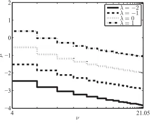
λ > λ. If this is the case, the one-armed bandit problem is called indexable [16]. Even if the state space is finite, proving indexability is likely to be highly involved [5]; we assume that it holds here as confirmed through extensive numerical experimentation (see for example Fig. 1).
The discount-optimal value function Vλ := sup
πVλ,π for
the one-armed problem with subsidy can be obtained us-ing value iteration (see Prop. 3.2). For the average re-ward case one can formulate a similar result stating that
Gλ:= sup
πGλ,π can be found fromrelative value iteration
as defined for example in [13, Section 8.5.5]. First we intro-duce the operatorT v:= maxa∈{0,1}Tav, where
Tav(μ, ν) :=
λ+β v(ϕ μ, ϕ2ν+σ2), a= 0, μ+β−∞∞ v(ϕ y, σ2)φμ,ν(y)dy, a= 1,
with φμ,ν denoting the normal density with mean μ and varianceν. Proofs can be found in the appendix.
Proposition 3.2. ForVλ
0 ≡0the iteration
Vnλ=T Vnλ−1 (8)
converges to a unique functionVλ: Ψ→Rasn→ ∞that satisfies the Bellman equation,
Vλ=T Vλ.
ThisVλ is the discount-optimal value function for the
one-arm bandit problem with subsidy λ. An optimal policy for this problem maps(μ, ν)to actionaifVλ(μ, ν) =T
aVλ(μ, ν).
Structural Properties.
Let us first consider monotonicity properties of the optimal value functionVλ.Lemma 3.3. Letϕ∈(0,1). ThenVλ(·, ν)is convex,
con-tinuous, non-decreasing, and not constant; and Vλ(μ,·) is
non-decreasing.
Fig. 1 and similar numerical experiments1suggest that the passive set Pλ and the active set Pc
λ are separated by a 1To execute the value iteration we truncate Ψ1to [−6σ,6σ],
and considerλ∈[−2σ,2σ]. Discretization is done in steps of size 0.01, which is preserved when truncating Ψ2.
switching curve(defined on the countable space Ψ2).
Assumption 1. It holds thatμ:= supμ|(μ, ν)∈ Pλ<
∞andμ:= infμ|(μ, ν)∈ Pλc>−∞.
We conjecture that this assumption generally holds here; it states that if the expected reward obtained when playing is large enough, then it is optimal to indeed play the arm, while if it is very small, we should rather take the subsidy. To see that there is a switching curve, it remains to be proven that in betweenμ andμ there are no μ1 < μ2 such that (μ1, ν)∈ Pλcand (μ2, ν)∈ Pλ.
4 21.05
−4 −3 −2 −1 0 1 2
ν
μ
λ=−2
λ=−1
λ= 0
λ= 1
Figure 1:Switching curves: below the curve the optimal action is passive, above it is active. β= 0.8,ϕ= 0.9,σ= 2.
Proposition 3.4. If Assumption 1 holds, then a policy that achieves the optimal value function Vλ is a threshold
policy: There exists a switching curve (sequence)ζλ: Ψ2→
Ψ1 such thatPλ={(μ, ν)|μ≤ζλ(ν)}.
Numerical evidence such as provided in Fig. 1 suggests that the switching curve is in fact strictly decreasing, i.e. it is optimal to give some priority to exploration.
Assumption 2. The switching curve is non-increasing.
It follows from the assumptions and Prop. 3.4 that the Whit-tle index is monotone.
Corollary 3.5. Provided Assumption 1 holds, the Whit-tle indexω(μ, ν)is non-decreasing inμ. If in addition As-sumption 2 holds, thenω(μ, ν)is non-decreasing inν.
Consequently, the Whittle index policy assigns compara-tively larger indices to arms that have not been activated for a longer time. In accordance with this observation, Fig. 2 shows that the correction term q(μ, ν) is positive and in-creases inν. It is larger forμclose to zero, which may be explained by noting that exploration is less important if|μ|
is large, for in that case there is less uncertainty about the direction in whichμwill evolve. Furthermore, we confirmed numerically that the slope ofζλ(ν) increases asβincreases as in this case exploration becomes more beneficial.
4 21.05
−4 −3 −2 −1 0 1 2 3 4
ν
μ
0.5 1 1.5 2
Figure 2: Correction termq(μ, ν)obtained for the Whit-tle index. β= 0.8,ϕ= 0.9,σ= 2.
3.2
Parametric Index
As no closed form for the Whittle index is available, the Whittle indices have to be computed and stored for every belief state in Ψ, while the evaluation of the optimal value function for the one-armed problem with subsidy is compu-tationally expensive. Therefore, instead of finding the index for the one-armed problem with subsidy that is optimal (the Whittle index), we propose to find the index that is optimal when restricting to a family of parametric functions. A sim-ple examsim-ple is obtained by picking a functionq(μ, ν) that is proportional toν, the most obvious measure for the decision maker’s uncertainty. This yields theparametric index
γ(μ, ν) =μ+θν, (9)
whereθ≥0 as motivated by Corollary 3.5. The correction term θν allows to adjust the priority the decision maker wants to give to exploration. We denote the associated pol-icy byπθ.
The parametric index can be related to the Whittle index as follows. Numerical experiments (such as Fig. 1 for dis-counted, and related experiments for average rewards) sug-gest that the optimal switching curve may be well approx-imated by a linear function, the slope of which is negative but does not depend on λ. The position of the curve on the other hand does depend onλ. Such an approximation is given byζλ(ν)≈ −θν+λ+cwithθ≥0, c∈R. Asζλ(ν) takes some valueμ∈R, solving forλ(which may correspond to the Whittle index) suggests using an index of the form (9), where without loss of generality we takec= 0.
In the next section we show that we can explicitly describe the asymptotic dynamics of the system induced byπθ.
4.
SYSTEM WITH MANY ARMS
We investigate the behavior of the system with many arms asd → ∞ and kd/d → ρ. Section 4.1 outlines the main idea: the limiting proportion of belief states remains stable in an equilibrium system with infinitely many arms. In Sec-tion 4.2 we relate the equilibrium system to a single arm process, and use this connection to propose an algorithm for performance evaluation. This algorithm is used to optimize
πθin Section 4.3.
4.1
Limiting Empirical Distribution
We first informally describe the intuition motivating this section. Consider the system withdarms as before, and to simplify the exposition suppose for now that the system is stationary. Let Γi(t) denote the process of indices associated
with armi, that is, Γi(t) :=γμi(t), νi(t). Note that the index processes Γi(t) and Γj(t),i, j= 1, . . . , d, are generally dependent because the belief states of both arms depend on the action that was chosen, which in turn depends on the index of all arms in the system (as they are coupled by the requirement that thosekarms with the largest indices are activated). Let us now focus on a single armiin this system and suppose that its belief state evolves fromψat timetto another belief stateψat timet+ 1. Whiledis small, this certainly changes the proportion of arms with current belief stateψconsiderably. However, ifdis very large, we should be able to find another armjwhose new belief state at time
tis (in close proximity to)ψ. It thus seems reasonable to ex-pect that, as we add more arms to the system, it approaches a mean-field limit in which the proportion of arms associ-ated with a certain belief state remains fixed. Thus, in the limit, the action chosen for a certain arm is independent of the current belief state of any other arm, as there is always the same proportion of arms associated with a certain belief state in the system.
Let us now more formally investigate the proportion of arms that are associated with a certain belief state at timet. We focus on parametric index functions as defined in (9). The empirical measure
Md(C, t) := 1
d d
i=1
1μi(t), νi(t)
∈C
(10)
quantifies the proportion of arms in thed-dimensional sys-tem whose belief state falls intoC∈ B(Ψ) at timet, where B(Ψ) denotes the Borelσ-algebra on Ψ. It is related to the measure on indices,
Md(B, t) := 1
d d
i=1
1Γi(t)∈B
(11)
withB∈ B(R), through
Md(B, t) =Md
(μ, ν)∈Ψ|μ+θν∈B
, t
. (12)
We examine the dynamics ofMd(C, t). To this end we enu-merate the elements in Ψ2, that is,ν(h)=σ2(1−ϕ2(h+1))/(1− ϕ2),h= 0,1,2. . ., so thath+ 1 is the number of time steps since an arm was played last. We refer tohas theageof an arm. Then (10) can be written as, withB∈ B(R),
∞
h=0
Mhd(B, t) :=
∞
h=0
1
d
i:νi(t)=ν(h)
1μi(t)∈B. (13)
Many-arms Asymptotics.
As motivated at the beginning of this section, it is reasonable to believe that the limit-ing proportion of arms associated with a certain belief state evolves deterministically, and thus, that the dynamics of the limiting system can be described by non-random measuresmh(·, t). For brevity we writemh(x, t) formh(−∞, x], t),
and denote by Φμ,ν the normal distribution function with
meanμand varianceν. We definemh(·, t) by the recursion
mh
x, t+ 1 (14)
= ⎧ ⎪ ⎨ ⎪ ⎩
∞
h=0
∞
h(t) Φz,ν(h)
x ϕ
mh(dz, t), h= 0,
mh−1
minx
ϕ, h−1(t)
, t
, h≥1,
whereh(t) :=(t)−θν(h)with(t) defined by
(t) = sup
∞
h=0
mh[,∞), t=ρ
. (15)
Here,mhdenotes the measure on indices, i.e.
mh(B, t) =mhμ∈Ψ1|μ+θν(h)∈B, t
, (16)
cf. Eqn. (12). Note that h(t) is a threshold such that at
timetthe policyπθactivates all arms that are of agehand
have conditional meanμ(t)≥h(t),h≥0. Obviously, if the policy is myopic, thenh(t) =(t) does not depend on the age of an arm and the above expressions can be simplified. Recursion (14) is obtained based on the dynamics of the belief states as given in (3). The evolution of m0(·, t) is determined by the evolution of the belief state of all arms that have been played in the previous time slot. Ifh >0 on the other hand, we use that arms of agehmust have been of ageh−1 at the previous decision time; and since they have not been activated, their mean must have been below the thresholdh(t−1).
For the (pre-limit) empirical processesMdit obviously holds
that Md(Ψ, t) = 1 as well as Md
0(Ψ1, t) = kd/d. These
properties carry over to the limiting measure.
Lemma 4.1. If the sequence{mh(B,0)}h satisfies
m0Ψ1,0=ρ, and
∞
h=0
mhΨ1,0= 1, (17)
then the same holds formh(B, t)for allt >0.
This is easily proven by induction using (14)–(16). We be-lieve that (14) indeed describes the mean-field behavior of the dynamical system:
Conjecture 1. Assume thatMd
h(B,0)converges weakly
tomh(B,0)for allh≥0,
Mhd(B,0)−→w mh(B,0),
asd→ ∞whilelimd→∞kd/d=ρ. Then, for allt, h≥0,
Mhd(B, t)−→w mh(B, t).
Long-run Equilibrium.
Note from (14) that forh≤twe can expressmh(B, t) in terms ofm0(B, t),mhx, t=m0
min
j=1,...,h
x ϕh,
h−j(t−j) ϕh−j
, t−h
.
Then the fixed-point equation corresponding to (14) is given by
m∗0x=
∞
h=0
∞
∗h
Φz,ν(h)
x ϕ
m∗h(dz)
=
∞
h=0
minj ∗h−j ϕh−j ∗h ϕh
Φϕhz,ν(h)
x ϕh
m∗0(dz)
wherej= 1, . . . , h. Here,∗h=∗−θν(h)where the steady
state∗ is defined by
∗= sup
∞
h=0
m∗h
[,∞)
=ρ
, (18)
andm∗again denotes the measure on indices, cf. (16).
The above system of equations describes possible equilib-rium points of the measure valued dynamical system. It is intricate due to the coupling of∗, m∗ and the measures
mh, h ≥0. Nevertheless, the system is elegant in that its
solution can potentially be described through a single mea-sure, namelym∗0.
For the special case ofθ= 0 (myopic) we verified numeri-cally that with arbitrary initial choice{mh(·,0)}satisfying (17) an equilibrium point satisfying (18) is indeed attracting. Furthermore, whendandtare large enough, the proportion of arms associated with a certain belief state in a simulated system withdarms is indeed fixed and well approximated by the solution to (18) when operated under the myopic policy.
4.2
The Equilibrium Index Process
We now relate the system with many arms operated under
πθ to a specialone-armed process with threshold. For this
process the arm is activated whenever the index exceeds a specified threshold, i.e. a(t) =1{μ(t) +θν(t)≥}. Be-cause the evolution of the belief state and thus the evolution of the index depends on, we denote the associated stochas-tic process of indices by Γ(t) :=μ(t) +θν(t).
Suppose that is picked in such a way that we activate with probabilityρ; denote it by. Then a policy π
θ that
chooses actionai(t) =1μi(t) +θνi(t)≥for every arm
iin an unconstrained system withdarms is a policy which activates ρ d arms on average (this is essentially the idea behind Whittle’s relaxation [16]). Thus, as d → ∞, the policyπ
θactivates approximately a proportionρof arms at
every decision time.
We believe that in steady state (ast → ∞ or under sta-tionarity) the equilibrium of the measure-valued dynamical system is directly related to the one-armed process with this particular threshold, and furtherequals∗of (18).
Conjecture 2. Assume that the index is parametric, and thatΓ(t)is stationary. Then the equation
PΓ(t)≥=ρ (19)
has a unique solution∗, which satisfies Eqn. (18), and
PΓ∗(t)∈B
=
∞
h=0
m∗h(B),∀B∈ B(R).
A practical implication of Conj. 1 and 2 combined is that in the limit, asd→ ∞andt→ ∞, a parametric index policy
πθis equivalent to the policy that activates armiin an un-constrained system whenever Γi(t)≥∗, where∗is defined
by (19). This motivates the following simple algorithm for performance evaluation.
Algorithm Performance evaluation.
1: For largeT determine∗ such thatT−1Tt=0ai(t) =ρis
achieved for a policyπ∗ θ .
2: Use the sample path of Step 1 to obtain an estimateGfor the expected average reward of the one-armed system. 3: OutputGd:=d Gas an approximation of the expected
aver-age reward of the multiarmed system withdarms operated underπθ.
The virtue of this algorithm is that the behavior of the many-armed system is approximated by simulating a much simpler one-armed problem.
4.3
Optimized Parametric Index
The algorithm can be used to approximate the best parame-ter values for a parametrized index policy. We approximate
θ∗:= arg maxθGd(θ) byθ∗ := arg maxθG(θ), whereGd(θ)
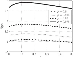
is the average reward obtained under πθ for the problem withdarms, andG(θ) is the estimator forG(θ) as obtained from Step 2 of the algorithm. Fig. 3 depicts the estimated expected average rewardG(θ) as a function ofθ. The figure suggests that for largeϕ, the myopic policy (which corre-sponds toθ= 0) can be improved significantly.
0 0.1 0.2 0.3 0.4 0.5
0.5 1 1.5 2 2.5 3
θ
¯G(
θ
)
ϕ= 0.9 ϕ= 0.925 ϕ= 0.96 ϕ= 0.975
Figure 3: Expected average reward G(θ) computed by the algorithm as a function of θ. σ = 2, ϕ ∈
{0.9,0.925,0.95,0.975},ρ= 0.4,T= 2×10⁶.
We now examine the performance ofπθwhen the parameter
is chosen to beθ∗. In contrast to the approximationGd(θ) that is obtained from the algorithm, we denote the estimated average reward obtained by Monte Carlo simulation of the
d-armed system byGd(θ). We defineθ∗d:= arg maxθGd(θ). Accordingly,Gdθ∗andGdθ∗dare the average rewards
obtained when simulating the system underπθ, whereθ is
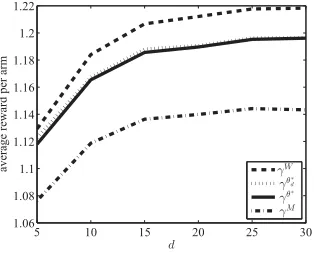
chosen asθ∗andθ∗drespectively. In Fig. 4 we compare these quantities to the average rewards obtained when simulating the system under the Whittle index and the myopic pol-icy. Unsurprisingly, the Whittle index policy outperforms the other index policies – in fact, we believe it to be asymp-totically optimal. However, the parametrized index does considerably better than the myopic.
Importantly, we note from Fig. 4 thatθ∗d is indeed well ap-proximated byθ∗. Thus, instead of optimizing the param-eter by simulating the multidimensional d-armed system, we can approximate the bestθ-value directly from the one-armed process with threshold for any value ofd(such that
kd=ρ d).
5 10 15 20 25 30
1.06 1.08 1.1 1.12 1.14 1.16 1.18 1.2 1.22
d
average reward per arm γW
γθ∗
d
γθ∗ γM
Figure 4: Comparison of average rewards achieved per arm under the Whittle, the parametric index (9) and the myopic policy. The parameterθis found by optimizing (i) the problem withd arms (dotted), and (ii) the one-armed problem. ϕ= 0.9,σ= 2,ρ= 0.4,T= 100,000.
5.
CONCLUDING REMARKS
This paper provides a starting point for a rigorous investi-gation of the structural properties and performance of index policies in partially observable restless bandit problems with AR(1) arms. This incorporates (i) the analysis of the Whit-tle index as a likely candidate for an asymptotically optimal policy asd→ ∞whilekd/d→ρ, and (ii) insights into the behavior of the system in this asymptotic regime. In addi-tion to our conjectures above, we also believe that some form of asymptotic independence holds for the index processes as the number of arms grows large. In this context we men-tion that Γi, i = 1, . . . , d, are exchangeable [2]. This may yield a path for proving asymptotic independence. The re-cursions on measures defining the limiting dynamical system can perhaps be treated along the lines of [10].
Furthermore, many of the ideas in this paper can be gener-alized. For example, the results obtained in Section 3.1 for discounted rewards similarly hold in the average reward case, and the assumptions made in that section generally hold for the problem we consider. Beyond that, we can extend the treatment to AR processes of higher order, heterogeneous arms and bandit problems with correlated arms.
6.
ACKNOWLEDGMENTS
This project is supported by the Australian Research Coun-cil grant DP130100156.
7.
REFERENCES
[1] R. Aguero, M. Garcia, and L. Munoz. Bear: A bursty error auto-regressive model for indoor wireless environments. InPIMRC, pages 1–5, 2007. [2] D. J. Aldous.Exchangeability and related topics.
Springer, 1985.
[3] K. Avrachenkov, L. Cottatellucci, and L. Maggi. Slow fading channel selection: A restless multi-armed bandit formulation. InISWCS, pages 1083–1087, 2012. [4] N. B¨auerle and U. Rieder.Markov Decision Processes
with Applications to Finance. Springer, 2011. [5] F. Cecchi and P. Jacko. Scheduling of users with
markovian time-varying transmission rates. InACM SIGMETRICS, pages 129–140, 2013.
[6] J. Gittins, K. Glazebrook, and R. Weber.Multi-armed Bandit Allocation Indices, second edition. Wiley, 2011. [7] K. Glazebrook, D. Hodge, C. Kirkbride, and R. Minty. Stochastic scheduling: A short history of index policies and new approaches to index generation for dynamic resource allocation.J. of Scheduling, pages 1–19, 2013. [8] K. Liu, R. Weber, and Q. Zhao. Indexability and
whittle index for restless bandit problems involving reset processes. InCDC-ECC, pages 7690–7696, 2011. [9] K. Liu and Q. Zhao. Indexability of restless bandit
problems and optimality of whittle index for dynamic multichannel access.Trans. on Info. Theory,
56:5547–5567, 2010.
[10] R. McVinish and P. Pollett. The limiting behaviour of a stochastic patch occupancy model.J. Math. Biol., 67:693–716, 2013.
[11] J. Ni˜no-Mora. A restless bandit marginal productivity index for opportunistic spectrum access with sensing errors. InNetwork Control and Optimization, pages 60–74. Springer, 2009.
[12] C. Papadimitriou and J. Tsitsiklis. The complexity of optimal queuing network control.Math. of Oper. Res., 24:293–305, 1999.
[13] M. Puterman.Markov decision processes: discrete stochastic dynamic programming. Wiley, 1994. [14] I. Verloop. Asymptotic optimal control of multi-class
restless bandits.CNRS Technical Report, hal-00743781, 2014.
[15] R. Weber and G. Weiss. On an index policy for restless bandits.J. of Appl. Prob., 27:637–648, 1990. [16] P. Whittle. Restless bandits: Activity allocation in a changing world.J. of Appl. Prob., 25:287–298, 1988.
APPENDIX
Proof of Lemma 2.1. For each armiwe have
Eμi,νi|Xi(t)| ≤Eμi,νi
ϕt|Xi(0)|+ t−1
j=0
ϕji|εi(t−j)|
≤
! 2νi
π +|μi|+
! 2
π
1
1−ϕ =:B(μi, νi),
which is finite, and thus,
sup
π ∞
t=0 βtEπμ
i,νi
d
i=1
|Xi(t)ai(t)|
≤dmaxiB(μi, νi)
1−β <∞,
whence supπVπ(μ,ν) is finite, and∞ t=0βt
d
i=1|Xi(t)ai(t)|
converges almost surely to a finite limit. The variables
ZT :=T t=0βt
d
i=1Xi(t)ai(t) thus converge almost surely
asT→ ∞and are dominated by the absolute sum which has finite mean. Hence, by dominated convergence Eπ
μ,νZT →
Eπ
μ,ν∞t=0βt
d
i=1Xi(t)ai(t) .
Proof of Proposition 3.2. Defineb(μ) := 1+μ2. Then, because|max{m, μ}| ≤1 +|m|b(μ), the absolute value of the expected immediate reward under both actions (passive, active) is bounded by1 +|m|b(μ) for any belief state in Ψ. Furthermore,
∞
−∞
b(ϕy)φμ,ν(y)dy≤
1 +ϕ2νmaxb(μ)
and hence,bis an upper bounding function in the sense of [4, Def. 7.1.2]. The implication of this is that the space V of measurable functions v: Ψ→R with finite weighted supremum norm defined by
vb:= sup
μ,ν
|v(μ, ν)|
b(μ) <∞
contains the optimal value functionV. We apply [4, Thm. 7.2.1]. To verify the main condition of the latter, define the operatorQby
Qv(μ, ν) :=
max
βv(ϕμ, ϕ2ν+σ2), β
∞
−∞
v(ϕy, σ2)φμ,ν(y)dy
.
Takeb(μ, ν) =b(μ) as defined above and observe that
Qnb(μ, ν)≤βn
1 +ϕ2νmax+ϕ2nν+μ2 ,
whenceQnb→0 asn→ ∞. Noting that the further regu-larity conditions of [4, Thm. 7.2.1] are satisfied, we obtain that with initial choiceV0≡0 the value iteration converges to an optimal value function, and an optimal policy exists; namely, it is optimal to take the action that maximizes the right-hand side of the Bellman equation. The uniqueness of the value function can be seen as follows. Letv andw be two fixed points ofT. Then
Tnv(μ, ν) =TTn−1v(μ, ν)=· · ·=v(μ, ν),
for everyn∈N. BecauseQn→0 we know that for every
(μ, ν) there existsnμ such that |Tnμv(μ, ν)−Tnμw(μ, ν)|
b(μ, ν) ≤αsupμ,ν
|v(μ, ν)−w(μ, ν)|
b(μ, ν)
for someα∈(0,1). Hence,
v−wb= sup
μ,ν
|Tnμv(μ, ν)−Tnμw(μ, ν)|
b(μ, ν) ≤αv−wb,
which implies thatv≡w.
Proof of Lemma 3.3. The proof is by induction on (8), and consists of three parts. Part (a) refers to the convexity
assertion, which implies continuity. In Part (b) we prove the monotonicity properties ofVm(·, ν) for fixedν, whereas in Part (c) we show monotonicity ofVm(μ,·) withμfixed.
(a) Suprema, expectations, compositions of convex and in-creasing functions as well as linear combinations with non-negative weights of convex functions are convex. Then the result follows from (8) by induction.
(b) For V0m ≡ 0, we have that V1m(·, ν) is non-decreasing and thus we may assume that Vm
n (·, ν) is non-decreasing
for some n. If μ1 ≤ μ2, then by the stochastic ordering of Yμi,ν ∼ N(μi, ν) it holds that E
Vm n
ϕ Yμ1,ν, σ2
"
≤
EVnmϕ Yμ2,ν, σ2
"
. It follows by induction that Vnm is non-decreasing inμfor alln∈N, and thus their limitVm
is non-decreasing in μ. Furthermore, since a lower bound forVmis given by the value obtained when always playing
active, μ/(1−ϕβ), which is strictly increasing in μ, it is evident thatVmcannot be constant inμ.
(c) LetVm
0 ≡0. ThenV1m(μ,·) is constant and thus
non-decreasing. Assume that Vnm(μ,·) is non-decreasing. We prove below that EVm
n
ϕ Yμ,ν, σ2" is non-decreasing in
ν. Then it follows by induction thatVm
n is non-decreasing
inν for everyn, and thus, so isVm.
For brevity we assume thatVm(·, ν) is differentiable. Define
g(y) :=Vm n (ϕ
√
νy+μ, σ2); this is increasing and convex as it is a composition of a convex and a monotone increasing function. Applying Jensen’s inequality we obtain
∂ ∂νE
Vnmϕ Yμ,ν, σ2"
= ϕ
2√ν
∞
−∞
y Vnmϕ√νy+μ, σ2φ0,1(y)dy
= ϕ
2√ν
∞
−∞
y g(y)φ0,1(y)dy
≥ ϕ 2√ν
∞
−∞
g(y)−g(0)φ0,1(y)dy≥0
becausegis convex (and thusg(b)−g(a)≤g(b)(b−a) for alla, binR, the domain ofg).
Proof of Proposition 3.4. Vm(·, ν) is non-decreasing
and convex by Lemma 3.3, and thus, the same holds for
TaVm,a= 0,1. By Assumption 1 both passive and active
set are non-empty, whenceT0Vm(·, ν) andT
1Vm(·, ν)
inter-sect. Since both functions are convex and increasing, they can intersect at most twice (if their paths are equal on a con-nected set of points, we refer to this as a single intersection). But since by assumptionT0Vm(μ, ν)≥T
1Vm(μ, ν) for all μ < μwhereasT1Vm(μ, ν)> T
0Vm(μ, ν) for allμ > μ, they
can only intersect exactly once, whence there is a unique switching point, which we denote byζm(ν). This argument
applies for everyν∈Ψ2.
Proof of Corollary 3.5. Letμ1≤μ2, then Prop. 3.4 implies (μ1, ν)∈ Pω(μ2,ν). Hence,ω(μ2, ν)∈ {m|(μ1, ν)∈ Pm}
and thus, ω(μ1, ν) ≤ω(μ2, ν) by definition of the Whittle index as an infimum. The monotonicity of ω(μ,·) follows along similar lines using Assumption 2.