RESEARCH
Prediction of environmental indicators
in land leveling using artificial intelligence
techniques
Isham Alzoubi
1*, Salim Almaliki
2and Farhad Mirzaei
3Abstract
Background: Land leveling is one of the most important steps in soil preparation and cultivation. Although land leveling with machines require considerable amount of energy, it delivers a suitable surface slope with minimal dete-rioration of the soil and damage to plants and other organisms in the soil. Notwithstanding, researchers during recent years have tried to reduce fossil fuel consumption and its deleterious side effects during this operation. The aim of this work was to determine the best linear model using Artificial Neural Network (ANN), Imperialist Competitive Algo-rithm–ANN, regression, and Adaptive Neural Fuzzy Inference System (ANFIS) to predict the environmental indicators for land leveling and to determine a model to estimate the dependence degree of parameters on each other. Methods: New techniques such as ANN, ICA, GWO–ANN, PSO–ANN, sensitivity analysis, regression, and ANFIS that using them for optimizing energy consumption will lead to a noticeable improvement in the environment. In this research, effects of various soil properties such as embankment volume, soil compressibility factor, specific grav-ity, moisture content, slope, sand percent, and soil swelling index in energy consumption were investigated. The study was consisted of 350 samples which were collected from 175 regions in two depths. The grid size was set 20 m × 20 m from a 70-ha farmland in Karaj province of Iran.
Results: The models that reveals the relationship between the land parameters and the energy indicators were extracted. As it was expected three parameters; density, soil compressibility factor and, embankment volume index had significant effect on fuel consumption. In comparison with ANN, all ICA–ANN models had higher accuracy in prediction according to their higher R2 value and lower RMSE value. Statistical factors of RMSE and R2 illustrate the superiority of ICA–ANN over other methods by values about 0.02 and 0.99, respectively. Results also revealed the superiority of integrated techniques over other methods for prediction of complicated problems such as land leveling energy estimation.
Conclusion: Results were extracted and statistical analysis was performed, and RMSE as well as coefficient of deter-mination, R2, of the models were determined as a criterion to compare selected models. According to the results,
10-8-3-1, 10-8-2-5-1, 10-5-8-10-1, and 10-6-4-1 MLP network structures were chosen as the best arrangements and were trained using Levenberg–Marquardt as NTF. Integrating ANN and imperialist competitive algorithm (ICA–ANN) had the best performance in prediction of output parameters, i.e., energy indicators.
Keywords: Artificial Neural Network, Energy, Environmental research, Imperialist competitive algorithm, ANFIS
© The Author(s) 2019. This article is distributed under the terms of the Creative Commons Attribution 4.0 International License (http://creat iveco mmons .org/licen ses/by/4.0/), which permits unrestricted use, distribution, and reproduction in any medium, provided you give appropriate credit to the original author(s) and the source, provide a link to the Creative Commons license, and indicate if changes were made. The Creative Commons Public Domain Dedication waiver (http://creat iveco mmons .org/ publi cdoma in/zero/1.0/) applies to the data made available in this article, unless otherwise stated.
Open Access
*Correspondence: [email protected]; [email protected]
1 Department of Surveying and Geometric Eng, Engineering Faculty,
University of Tehran, Tehran, Iran
Introduction
During the last century due to increasing human popu-lation, demands for agricultural commodities have been enormously increased. Nowadays, one of the cardinal environmental challenges in the world is energy produc-tion and consumpproduc-tion. Despite soft growth of renew-able energy usage such as solar energy, inappropriate use and lack of proper management have led to an intensive rise in fossil fuel energy consumption in this field. It also should be taken into the account that environmental con-servation and market globalization will be dependent on food security in the future agriculture [1]. Regarding this, some special policies should be addressed to consider energy viewpoint in conjunction with the environmental issues to solve the problem. Land leveling is one of the heaviest and costly operations among agricultural prac-tices that consume considerable amount of energy. In addition, moving heavy machines on the ground makes the soil denser, particularly in the wet regions where the moisture content of the soil is high and it makes a situ-ation that is not easily recoverable [2–4]. On the other hand, land leveling simplifies the irrigation, improves field situations in other practices related to agriculture and regulates the soil surface and normalizes its slope [5]. Reportedly, there are three significant factors which have effect on grain yield including the effects of land lev-eling, methods of water application and the interaction between land leveling and water applied. Okasha et al. observed a noteworthy connection between slope and diverse irrigation scheme in different seasons [2]. Some researchers have used other techniques such as Internet of Things (IoT) to optimize the irrigation process based on the physical characteristics of soil [6]. However, these methods do not engage in land leveling process. Diverse methods of land leveling can affect the physical and chemical properties of the soil, and hence can make dif-ferences in plant establishment, root growth, aerial cover and eventually crop yield. As a direct result, one of the most important steps in soil preparation and a key fac-tor in food production that should be optimized is land leveling [5]. Besides, decreasing fossil fuel consump-tion for land leveling diminishes air contaminants and improves the environmental condition. There is a grow-ing understandgrow-ing of importance and effects of water and soil management which in turn reveals the significance of optimized laser land leveling from social, financial and agronomic points of view [7]. Even though some improv-ing strategies have been proposed for the enhancement of operations related to the environment, they have diverse undesirable effects [8]. Using computers and the Internet has shown a great potential to solve these types of problems by reducing the aforementioned undesirable effects. There are myriad of computer-based techniques
Impact Assessment (EIA) was also addressed in litera-ture which involves the investigation and estimation of scheduled events with a view to ensure environmentally sound and sustainable improvements [8]. Since, land lev-eling with machines requires considerable energy, thus, optimizing energy consumption in the leveling operation is expected. As a result, here, five approaches including ANN, integrating Artificial Neural Network and Impe-rialist competitive algorithm (ICA–ANN) and Sensitiv-ity Analysis, Regression, ANFIS models have been tested and evaluated in prediction of environmental indicators for land leveling. Moreover, since a limited number of studies associated with the energy consumption in land leveling have been done, the objective of current energy and cost research is to find a function for all the indices of the land leveling including the slope, coefficient of swell-ing, the density of the soil, soil moisture, special weight dirt and the swelling.
Materials and methods Case study region
To verify the accuracy and applicability of the proposed linear model, a case study was carried out based on requirements of the project in a farmland at Karaj, Iran. The farm area was 70 ha and was located in west of Karaj, 31°28′42″ north latitude and 48°53′29″ east longitude. Topographic maps of the farm were plotted at scale of 1:500. Length, width and height of points from a refer-ence point (coordinates of x, y and z) were considered as outputs. The grid size in the case study region was 20 × 20 m during topography operations. Samples were collected from the canters of each grid and two different depths; surface soil (0–10 cm) and subsurface soil (10– 30 cm). Totally, 350 samples (175 grid cells multiplied by 2 depths) were collected. In the laboratory, collected moist soil samples were firstly sieved through 10-mm mesh sieve to remove gravel, small stones and coarse roots and plant remnants; then passed through 2-mm sieve. Then, the sieved samples were dried at room tem-perature and moisture content of the samples as well as texture, bulk density, land slope and soil optimum density were determined.
Development of the ANN model
ANNs are massively parallel-distributed information processors that have certain performance characteristics resembling biological neural networks of human brain [29]. They have been developed as a generalization of mathematical models of human biological neural system [18]. There are a lot of structure types of ANN models. In this study, a typical feed-forward back propagation (BP) MLP structure was used. The main advantage of MLP structures over other types is that they have the
ability to learn complex relationships between input and output patterns, which would be difficult to model with conventional algorithmic methods [30]. An ANN struc-ture usually consists of an input layer, followed by one or more hidden layers and an output layer. The input nodes are the previous lagged observations, while the output provides the forecast for the future value. Hidden nodes with appropriate nonlinear transfer functions are used to process the information received by the input nodes. The model can be written as follows [28]:
where m is the number of input nodes, n is the number of hidden nodes, αj denotes the vector of weights from the
hidden to output nodes and βij denote the weights from
the input to hidden nodes. α0 and β0j represent weights
of arcs leading from the bias terms which have values always equal to 1 and f is a sigmoid transfer function [31]. Multiple layers of neurons with nonlinear transfer func-tions allow the network to learn nonlinear and linear relationships between input and output parameters [32]. The linear output layer lets the network to take any val-ues even outside the range of − 1 to + 1; while if the last
layer of a multilayer network has sigmoid neurons, then the outputs of the network will be only in a limited range [33]. Input variables were: specific gravity, density, mois-ture content, slope, inflation rate and type of the cut soil. Relevantly, output variables were: fuel energy, machinery energy, labor power, total cost and energy consumption. In this study, all available data sets were used for regres-sion modeling, but for ANN model development, data were randomly divided into three groups: 70% for train-ing the network, 15% for model cross validation and, 15% for testing [30]. Several architectures for type of MLP have been investigated to find the one that could result in the best overall performance. The learning rules of Momentum and Levenberg–Marquardt were considered and no transfer function for the first layer was used. For the hidden layers, the sigmoid and hyperbolic tangent transfer functions were applied, and for the last one a lin-ear transfer function was set. Also, a number of different network sizes and learning parameters have been tried.
As it is mentioned earlier, the ANN system applied for the predictor models had seven inputs; soil cut/ fill volume, soil compressibility factor, specific gravity, moisture content, slope, sand percent, and soil swell-ing index. On the other side, the outputs of each model were labor energy, fuel energy, total machinery cost, total machinery energy.
(1) yt = α0 +
n
j=1 αjf
m
i=1
βijyt−i + β0j+ εt
,
Since the main elements of ANNs are constituted by artificial neurons, the input model consists of dendritic nodes similar to a biological cell that could be repre-sented as a vector with N items X= (X1, X2,…, Xn); the
summation of inputs multiplied by their corresponding weights could be represented by scalar quantity S.
where W= (W1, W2,…,WN) is the weight vector of
asso-ciations among neurons. The S quantity is then passed to a non-linear activation function f, yielding the following output:
Non-linear transfer function is usually represented as sigmoid functions and is defined via:
The output of y can be the final result of the model or that of the previous layer (in multilayer networks). In the design of an ANN, certain elements should be taken into the account including type of input param-eters. In this research, three-layer perceptron network was used which is composed of an input layer and an output layer plus one hidden layer of computational modes. In each layer, a number of neurons were consid-ered which were connected to the neurons of neighbor-ing neurons via some associations. In these networks, the effective input of each neuron was as a result of the multiplication of the outputs of the previous neurons by the weights of those neurons. Neurons in the first layer receive the input information and transfer it to hidden neurons through related connections. The input signal in such networks is only expanded in a forward direction. The main advantage of such a network is the simplicity in implementing the model and estimating input/output data. Some of the major shortcomings of this model are the low training rate and need for a huge set of data.
Imperialist competitive algorithm (ICA)
ICA is a novel swarm-intelligence method that has been developed by mimicking the human being’s socio-politi-cal evolution strategies. ICA optimization process starts with initialization of random populations and some incipient empires. In each stage of ICA, a union of sub-groups, colonies, and imperialists assemble the empires. ICA breaks the early population into the subpopulations, and then it searches the solution space for the best point using two main operators: competition and assimilation. (2) S=
n
k=1 WkXk,
(3) y=f(s).
(4)
f(s)= 1
1+e−s.
During algorithm proceedings, empires can interact with the members of the swarm. Throughout the assimilation procedure, colonies move towards the relevant imperialist progressively. Imperialistic competition among the empires is the momentous procedure of the ICA [12, 19–21]. In competition stage, powerless empires collapse; whereas, the dominant ones gain further control over their colonies. This operation is stopped whenever one empire controls the entire countries. In termination condition, empire has equal cost with its colonies, which can be regarded as a sat-isfactory solution for the problem. To explain the algorithm more practically, the required steps are as follows: Step 1: Initializing phase. Scattering the early population randomly over the search space and composing the basic solutions in the format of a 1 ×Nvar array via Eq. (5):
where pi represents variables that are fundamentally
related to socio-political characteristics of the countries such as culture, language, religion, and economic policy. Nvar shows the total variables of the target problem. Step 2: computing the cost of every country using Eq. (6):
Step 3: Initializing the empires. The normalized cost of an imperialist is obtained via Eq. (7)
where fcost(imp,n) stands for the cost of nth imperialist, and NCn indicates its normalized cost.
p 4: Dividing the colonies among imperialists. This pro-cess is based on the power of imperialist and relationships between the countries and their interdependent empires (i.e., the countries should be possessed by their imperialist based on the power). This step is completed using Eqs. (8–
10), respectively:
where Powern is the normalized power of each
imperial-ist, Ncol and Nimp are the given number of colonies and imperialists, respectively, and NOCn represents the total
number of colonies that are possessed by nth empire. Step 5: Assimilation strategy. The purpose of the assimila-tion procedure can be expressed as the movement of the colonies towards their interdependent imperialist. Based (5) country = [p1,p2, p3,. . ., pNvar],
(6) C= f(country)=f(p1,p2,. . .,pNvar)
(7) NCn=fcost(imp,n)−max
i
fcost(imp,i)
,
(8)
Powern=
NCn Nimp
i=1 NCi
, (9) NOCn=round{Powern,Ncol},
(10)
on this stage, each movement is performed according to Eq. (11):
where x is a random number with uniform (or any
proper) distribution, β is a number greater than 1, and d is the distance between a colony and related imperi-alist. Step 6: Revolution strategy. In this strategy, a ran-dom amount of deviation is added to direct the colonies movement via Eq. (12):
where θ is a random variable with uniform distribution, and γ shows a parameter for adjusting the deviation from the initial movement direction. Step 7: Exchanging phase. During assimilation, whenever a colony reaches to a position with lower (better) cost compared with the imperialist, the imperialist and the colony exchange their positions, and the colony becomes new imperi-alist and vice versa. Step 8: Imperiimperi-alistic competition phase. Calculating the overall power of an empire that is mainly affected by the power of empire and its colonies as Eq. (13):
where TCn represents the total cost of the nth empire,
and ζ is a coefficient between 0 and 1 for decreasing the effect of colonies cost. Step 9: Imperialistic competi-tion strategy. Based on this process, each empire tries to extend its power to possess more colonies compared with other empires. Throughout the competition, weakest col-ony from the weakest empire is selected to be governed by the strongest empire. Imperialistic competition con-ducts a searching procedure towards a peak solution. The competition operator is designed to dedicate the colonies of the weakest empires to other empires. Based on TCn,
the normalized total cost is evaluated using Eq. (14):
where NTCn is the total normalized cost of nth empire.
According to NTCn, the possession probability of each
empire is computed with Eq. (15):
To find out the winner of competition with less com-putational effort, the vectors P, R, and D are formed via Eqs. (16, 17, 18):
(11)
x≈U(0,β×d) β >1,
(12) θ ≈U(−γ,γ )
(13)
TCn=fcost(imp,n)+ξ· NCn
i=1 f
(col,i)
cost
NCn ,
(14) NTCn=TCn−max
i
{TCi},
(15) Ppn= NTCn Nimp
i=1 NTCi (16) P= [PP1,PP2,. . .,PPNimp]
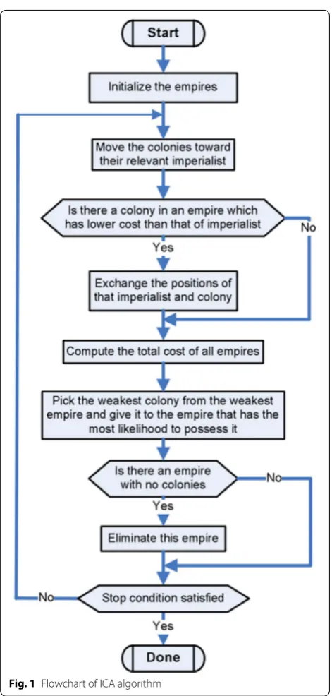
where P is the vector of possession probability of the imperialists and R represents a vector with uniformly distributed random values. Maximum index of D deter-mines the winner empire of the competition. Step 10: Eliminating phase. When a powerless empire loses all of its controlled colonies, it should be removed from the competition. Step 11: Convergence phase. Finally, the most powerful imperialist controls all the remained colo-nies. In such a condition, the algorithm is stopped. These steps can be shown in an algorithmic flowchart such as Fig. 1.
Training of ANNs can be done using the ICA. For this purpose, the algorithm should be able to adjust the weights and bias, so that the difference between the out-put of ICA and real outout-put be minimized. Mean squared error (MSE) was considered to determine the error.
Integrating Imperialist competitive algorithm and Artificial Neural Network (ICA–ANN)
In this study, after applying commands of ANNs in MAT-LAB software, the number of neurons in the input layer considered the same as the number of effective param-eters: Cut-Fill Volume (V) (embankment volume), soil compressibility factor, specific gravity, moisture content, slope, sand percent, and soil swelling index. Similarly, the number of neurons in the output layer should be equal to the number of desired parameters for modeling. Instead of the default commands for network training, ICA was used. For running ANNs, 70% of the data were used for training, 15% for evaluation, and the remained 15% were used for the test section.
Results
Sensitivity analysis model
The outputs that are shown in Table 1 are the results of the model after running for 500 times. Table 1 indicates meaningful F-values and a great significance (α < 0.0001) for all developed sensitivity analysis models that reject the null hypothesis clearly.
Figure 2 shows the sensitivity analysis for labor energy (LE). In this figure, F1–F7 represent land slope, moisture content, density, soil compressibility factor, embankment volume, Soil Swelling Index, and sand percent, respec-tively. The results revealed that F3 (density), F4 (soil com-pressibility factor), and F5 (embankment volume) had the highest sensitivities on LE.
(17) R= [r1,r2,. . .,rNimp]r1,r2,r3,. . .,rNimp ≈U(0, 1)
(18)
D=P−R= [PR] = [D1,D2,...,DN
imp]
= [PP1−r1,PP2−r2,...,PP
Sensitivity analysis also showed that three soil param-eters including; volume of soil, specific gravity and soil compaction had the greatest impact on the amount of energy required for land leveling. These parameters had direct relation with the required energy. In other words, more density of the soil leads to more required energy for constant volume of the soil. For a soil with higher den-sities, in addition to its weight, handling it also requires more energy consumption. It is obvious that more work-ing time of the machine leads to higher energy consump-tions. In the same manner, the higher the excavation volume, the greater the energy consumption. It can be interpreted in this way that more soil volume needs more time of machine and leads to more fuel consump-tion. Table 1 shows that soil volume is the most impor-tant parameter between all input variables for energy consumption including LE, FE, TMC and TME. It is clear that by increasing cut soil volume, needed time of machinery used increases, and consequently fuel energy increases as well. Furthermore, prolonged working time of machinery increases labor requirement for opera-tion which in turn raises the energy consumpopera-tion by the labors. On the other hand by decreasing the cut soil vol-ume, required human labor also decreases. Therefore, one of the most important ways for decreasing energy consumption is to reduce soil cut/fill. In addition, in each table, if the F value of a variable is higher than others, it indicates the higher impact of that variable in the final model. This situation has occurred for cut-fill volume as a variable which is the most effective factor and affects all responses of interest. In the same manner, the lower F value of a variable indicates lower impact of that variable on responses.
Regression model
Since the F-values of all models, that are shown in Table 2, indicated a great significance (α < 0.0001) for all developed regression models, the null hypothesis has rejected. Likewise, all models have significant P values as well.
Of the seven parameters of soil and land characteristics (moisture, density, soil compressibility factor, land slope, soil type, embankment volume), two factors: embank-ment volume and soil compressibility have the most sig-nificant effect on LE in land leveling. The factors of slope, V and soil type (sand) have significant effects on FE. V, soil compressibility factor and slope have significant effects on TMC in land leveling (Table 2).
Moreover, the results show that the effect of the land slope, swelling coefficient and soil type on energy con-sumption in land leveling is significant. By increas-ing land slope, volume of excavation and embankment
increases and the number of sweep and distance traveled by leveling machines also increases and fuel consump-tion will increase which is obvious. Increase in soil swell-ing factor increases the volume of the embankment and increase in volume of the embankment also increases the demand of fuel and energy. The fitted nonlinear equa-tions for the all response of interest including LE, FE, TMC, and TME are represented in Eqs. 19–22, respec-tively, in which the coefficients are provided in coded units. The coded equation is more easily interpreted. The coefficients in the actual equation compensate for
the differences in the ranges of the factors as well as the differences in the effects. Finally, LE, TMC, and TME were affected significantly only by three variables includ-ing: land slope, volume of the embankment (V), and soil swelling index (SSI). For FE model, the effect of SSI is not significant; however, soil percent has taken its place and affects the FE significantly. Labor energy consumption in land leveling is a nonlinear function of the soil com-pressibility factor and slope (Eq. 19). In the same way, fuel energy consumption in land leveling is also a nonlin-ear function of the soil compressibility factor and slope (Eq. 20). This is true for TMC and TME as well which have been represented in Eqs. 21 and 22, respectively. The value of each coefficient variable in the equation rep-resents the effect of variable on the function.
(19) (LE)0.8=34,161.36+3639.90∗Slope
+31,173.94∗V+911.96∗SSI
A relatively flat line shows insensitivity to change in that particular factor. The response trace plot for the LE, FE, TMC and TME was sketched. At this plot, the verti-cal axis is the predicted values and the horizontal axis is the incremental change made in factors included in the final equation model. The scatter plots of actual values of response of interest vs. predicted values using final models are displayed in Fig. 3a, b. The strong nonlinear (20) (FE)0.8=4.148
5+49,590.44∗Slope
+3.7825∗V−10,008.33∗Sand
(21) (TMC)0.8=3.319
8+3.5877∗Slope
+3.0158∗V+8.3936∗SSI
(22)
(TME)0.8=2.494
7+2.6216∗Slope
+2.2777∗V+6.7875∗SSI
Table 1 Analysis of variance for labor energy (LE), fuel energy (FE), total machinery cost (TMC), total machinery energy (TME)
Model Source Sum of squares df Mean square F value P value Prob > F
LE model Model 2.8587 1 2.8587 4277.61 < 0.0001
Cut-fill volume (V) 2.8587 1 2.8587 4277.61 < 0.0001
FE model Model 6.4788 1 6.4788 3931.00 < 0.0001
Cut-fill volume (V) 6.4788 1 6.4788 3931.00 < 0.0001
TMC model Model 2.73712 1 2.73712 4023.17 < 0.0001
Cut-fill volume (V) 2.73712 1 2.73712 4023.17 < 0.0001
TME model Model 1.08611 1 1.08611 4311.77 < 0.0001
Cut-fill volume (V) 1.08611 1 1.08611 4311.77 < 0.0001
0 20000 40000 60000 80000 100000 120000 140000 160000
F1 F2 F3 F4 F5 F6 F7
Sensivity
Feature vectors
Sensivity About the Mean
OUT1
effect of cut-fill volume on all the responses of interest is conspicuous (Fig. 3a, b). Figure 4 shows that energy and cost direct relationship with cut-fill volume as the major effect. All responses of interest are moderately affected by slope. Additionally, it is perceived that the increase of the slope led to increased energy and cost. The most appro-priate power transformation (lambda) for responses is detected by the Box–Cox diagram that results the mini-mum residual sum of squares in the transformed model (Fig. 3a). Scatter plots of actual vs. predicted values for regression model are shown in Fig. 4a–d.
Results of ANFIS model prediction
In this section, the results of ANFIS models for predic-tion of LE, FE, TMC, and TME are presented. MAT-LAB programming language was used for implementing ANFIS simulations. Different ANFIS structures were tried using the programming code and the appropriate representations were determined. Each structure for cor-respond combination has been evaluated using 100 inde-pendent runs and the statistical criteria (R2 and MSE) of the output models have been calculated for responses of interest. In Tables 3 and 4 the minimum, average and Table 2 Analysis of variance for labor energy (LE), fuel energy (FE), total machinery cost (TMC), total machinery energy (TME) models
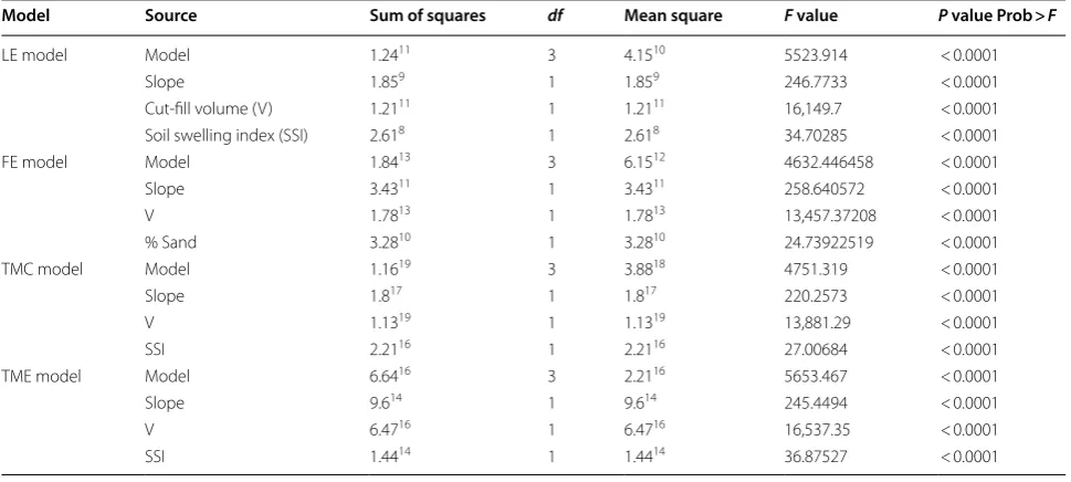
Model Source Sum of squares df Mean square F value P value Prob > F
LE model Model 1.2411 3 4.1510 5523.914 < 0.0001
Slope 1.859 1 1.859 246.7733 < 0.0001
Cut-fill volume (V) 1.2111 1 1.2111 16,149.7 < 0.0001
Soil swelling index (SSI) 2.618 1 2.618 34.70285 < 0.0001
FE model Model 1.8413 3 6.1512 4632.446458 < 0.0001
Slope 3.4311 1 3.4311 258.640572 < 0.0001
V 1.7813 1 1.7813 13,457.37208 < 0.0001
% Sand 3.2810 1 3.2810 24.73922519 < 0.0001
TMC model Model 1.1619 3 3.8818 4751.319 < 0.0001
Slope 1.817 1 1.817 220.2573 < 0.0001
V 1.1319 1 1.1319 13,881.29 < 0.0001
SSI 2.2116 1 2.2116 27.00684 < 0.0001
TME model Model 6.6416 3 2.2116 5653.467 < 0.0001
Slope 9.614 1 9.614 245.4494 < 0.0001
V 6.4716 1 6.4716 16,537.35 < 0.0001
SSI 1.4414 1 1.4414 36.87527 < 0.0001
maximum values of R2 and MSE for various combina-tions of developed ANFIS-based models are presented. Additionally, calculated R2 and MSE values of different developed models of labor energy vs. number of clus-ters are illustrated as well. It is worthwhile to mention that other outputs had similar behaviour. As presented in Table 3, statistical criteria for prediction of LE reveal that FIS model is superior to ANN-back propagation model. Average R2 value in FIS model for prediction of LE was found to be 0.9948 and 0.9944 in Mamdani and Sugeno models, respectively; while in back propagation model,
it was calculated as 0.9921. Moreover, as presented in Table 3, statistical criteria for prediction of FE reveal that FIS model are superior to ANN-back propagation model. Average R2 value in FIS model for prediction of fuel energy was found to be 0.9927 and 0.9922 in Mamdani and Sugeno models, respectively. While in back propaga-tion model, R2 value was calculated as 0.9891 and 0.9892, respectively.
value in FIS model for prediction of total machinery cost was found to be 0.9921 and 0.9922 in Mamdani and Sugeno models, respectively. While in back propagation model, R2 value was calculated as 0.9894 and 0.9895, respectively. As presented in Table 4, statistical factors for prediction of TMC indicate that FIS model perform better than ANN-back propagation model. Average R2 value in FIS model for prediction of TME was found to be 0.9950 and 0.9952 in Mamdani and Sugeno models, respectively; while in back propagation model, it was cal-culated as 0.9925 and 0.9926, respectively.
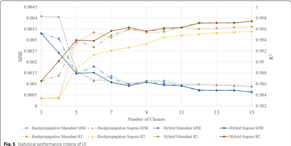
Determining the effect of number of clusters on all the developed models is feasible (Fig. 5). Moreover, com-parison between different optimization methods and FIS types can also be done. For the ANFIS-based model, in both training methods, the MSE (R2) value decreases (increases) and the prediction performance of devel-oped ANFIS-based models improves gradually with the
number of clusters. In addition, comparison of the results indicates that the Hybrid method has a higher value of R2 and a lower value of MSE; so that its results are more accurate. Also, the performance of the Sugeno FIS type was found to be better than that of Mamdani.
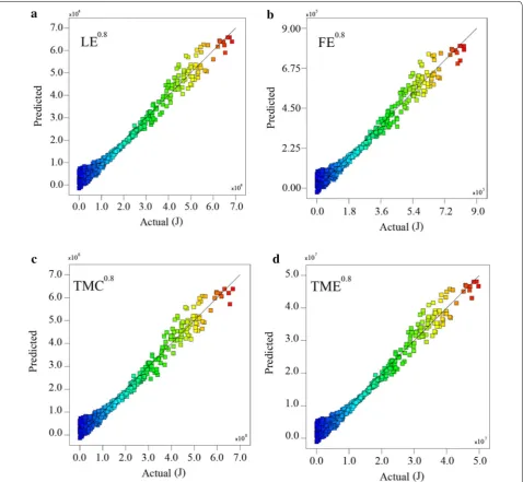
Comparison results of the predicted values of ANFIS models with actual data are shown in Fig. 6a–d. These predicted values are compared with actual data to show the performance of the ANFIS models for prediction of each response. Results from these figures reveal that FIS model is superior to ANN model in predicting LE, FE, TMC, and TME.
ANN model
The results of regression models and training various networks with different structures are presented in this section. The ANN models were developed by training the networks with various combination of Network Training Table 3 Calculated statistical criteria for prediction of labor energy using/fuel energy different combination of optimization methods and FIS types
Optimization method FIS type MSE R2
Min. Ave. Max. Min. Ave. Max.
Labor E.
Hybrid Mamdani 0.00063 0.00130 0.00329 0.9856 0.9948 0.9971
Sugeno 0.00058 0.00126 0.00326 0.9865 0.9944 0.9974
Back propagation Mamdani 0.00083 0.00102 0.00412 0.9831 0.9921 0.9965
Sugeno 0.00088 0.00154 0.00407 0.9831 0.9921 0.9964
Fuel E.
Hybrid Mamdani 0.00119 0.00181 0.00371 0.9851 0.9927 0.9952
Sugeno 0.00111 0.00173 0.00390 0.9843 0.9922 0.9955
Back propagation Mamdani 0.00119 0.00270 0.00560 0.9775 0.9891 0.9952
Sugeno 0.00123 0.00268 0.00560 0.9775 0.9892 0.9950
Table 4 Calculated statistical criteria for prediction of total machinery cost/energy using different combination of optimization methods and FIS types
Optimization method Fis type MSE R2
Min. Ave. Max. Min. Ave. Max.
Cost
Hybrid Mamdani 0.00122 0.00188 0.00387 0.9837 0.9921 0.9949
Sugeno 0.00119 0.00185 0.00394 0.9834 0.9922 0.9950
Back propagation Mamdani 0.00140 0.00251 0.00465 0.9805 0.9894 0.9941
Sugeno 0.00141 0.00250 0.00465 0.9805 0.9895 0.9940
Energy
Hybrid Mamdani 0.00059 0.00121 0.00353 0.9856 0.9950 0.9975
Sugeno 0.00058 0.00120 0.00356 0.9855 0.9952 0.9976
Back propagation Mamdani 0.00077 0.00183 0.00395 0.9839 0.9925 0.9968
Functions (NTF), number of hidden layers and number of neurons in the each hidden layer. For selecting the best network topology, totally 20,678 different ANN models were evaluated, and the RMSE and coefficient of deter-mination (R2) values were calculated. For a full compari-son between the performances of the trained structures, Tables 5 and 6 represent results obtained from ANN of feed-forward BP type with 7 different network training algorithms. These methods of training are available in the Neural Network Toolbox software and they use gradient- or Jacobian-based methods including Levenberg–Mar-quardt (trainlm), Bayesian regularization (trainbr), scaled conjugate gradient (trainscg), resilient BP (trainrp), gra-dient descent with momentum and adaptive learning rate BP (traingdx), Gradient descent with adaptive learning rate BP (traingda), gradient descent with momentum BP (traingdm) and conjugate gradient function (traincgf). These networks use 10 input data in the input layer to predict the outputs and utilize a linear function in their output layer to transfer the data to the output. The out-puts of the model represented in Tables 2 and 3 are the results of 500 thousand runs of the model. The selected NTFs for LE in land leveling, as shown in the first row of the Table 5, were the best because they had the highest correlation coefficient and lowest RMSE. These functions had 8 neurons in the first layer, and three neurons in the second. Details of the best trained networks for predic-tion of LE are shown in Table 5. The NTF of trainlm had higher RMSE and lower R2 for 2 (8-3) and 3 (2-7-6) hid-den layers but NTF of trainbr for 1 hidhid-den layer had the
best statistical interpretation. The NTF of trainlm includ-ing 2 neurons in one hidden layer is the simplest ANN for forecasting the LE with RMSE lower than 0.021 and R2 higher than 0.996. Details of the selected networks for prediction of FE are presented in Table 5. The NTF of trainlm had higher RMSE and lower R2 for 2 (4-2) and 3 (8-2-5) hidden layers but NTF of trainscg for 1 hidden layer had the best statistical output. The NTF of trainlm including 2 neurons in one hidden layer was the sim-plest ANN for predicting the FE with RMSE of lower than 0.033 and R2 higher than 0.995. As it is shown in the Table 6, the first model consisting of three hidden layers (5-8-10 topology) had the highest coefficient of determi-nation (0.9966) and the lowest values of RMSE (0.0287) indicating that this model can predict the TMC accu-rately. So, this model was selected as the best solution for estimating the TMC. The detail of the selected networks for prediction of TME is presented in Table 6. The NTF of trainlm had higher RMSE and lower R2 for 2 (6-4) and 3 (4-5-3) hidden layers. However, NTF of trainscg for 1 hidden layer had the best statistical results. For forecast-ing the FE, the NTF of traforecast-ingdx includforecast-ing 2 neurons in one hidden layer was the simplest ANN. The RMSE for this model was found to be 0.225 which was very low.
models in prediction of the targets. For a perfect fit, the data should fall along a 45-degree line, where the net-work outputs are equal to the targets. The training record was used to plot the training, validation, and test perfor-mance of the training progress (error vs. number of train-ing epochs).
Integrating Artificial Neural Network and Imperialist competitive algorithm (ICA–ANN) model
each response totally 18,000 networks were trained and evaluated. After several repetitions, the RMSE and coef-ficient of determination (R2) values were calculated. The network utilized a tansig function in its output layer to transfer the data to the output. The results obtained from the best trained models and their characteristics are illus-trated in Table 8. R2 value for prediction of LE was found to be 0.9987 and FE was predicted by R2 value of 0.9975. Using a network topology of 2-layer structure, TMC was
predicted by R2 value of 0.9963. While, R2 value for pre-diction of TME was found to be 0.9987. Scatter plots of Actual versus Predicted results of the ANN Models are shown in Fig. 8a–d. As the predicted values come closer to the actual values, the points on the scatterplot fall closer around the regression result (the diagonal line). These models can predict the target accurately and that is evident from closeness of the points to the line. For a perfect fit, the data should fall along a 45-degree line, Table 5 Selected ANN for prediction of labor energy (LE), fuel energy (FE)
Selected ANN for prediction of labor energy (LE) Selected ANN for prediction of fuel energy (FE)
NTF Network
topology RMSE R
2 NTF Network topology RMSE R2
trainlm 8-3 0.0159 0.9990 trainlm 8-2-5 0.0206 0.9983
trainlm 4-9 0.0159 0.9990 trainlm 10-4-10 0.0224 0.9980
trainlm 2-7-6 0.0164 0.9989 trainlm 4-2 0.0238 0.9977
trainlm 7-10 0.0164 0.9989 trainlm 9-2-3 0.0241 0.9977
trainlm 5-3 0.0165 0.9989 trainlm 5-2-9 0.0248 0.9976
trainlm 9-5-6 0.0166 0.9989 trainlm 3-2 0.0253 0.9974
trainlm 6-2-3 0.0167 0.9989 trainlm 2-2-2 0.0269 0.9971
trainlm 7-2-3 0.0171 0.9988 trainlm 2-2 0.0271 0.9971
trainbr 3-2 0.0174 0.9988 trainbr 2-6 0.0279 0.9969
trainbr 10-7 0.0179 0.9987 trainlm 6-2-2 0.0310 0.9962
trainbr 4 0.0171 0.9988 trainbr 5 0.0249 0.9975
trainlm 2 0.0209 0.9982 trainlm 6 0.0255 0.9980
traincg 6 0.0217 0.9981 trainscg 11 0.0261 0.9973
trainrp 7 0.0254 0.9974 traingdx 3 0.0329 0.9957
traingdx 2 0.0298 0.9964
Table 6 Selected ANN for prediction of total machinery cost (TMC), total machinery energy (TME)
Selected ANN for prediction of total machinery cost (TMC) Selected ANN for prediction of total machinery energy (TME)
NTF Network topology RMSE R2 NTF Network topology RMSE R2
trainlm 5-8-10 0.0287 0.9966 trainlm 6-4 0.0157 0.9990
trainlm 7-9-2 0.0298 0.9963 trainlm 4-5-3 0.0158 0.9990
trainlm 4-5-7 0.0304 0.9961 trainlm 6-2-4 0.0160 0.9990
trainlm 7-8 0.0329 0.9957 trainlm 2-7 0.0163 0.9989
trainlm 7-2-2 0.0332 0.9954 trainlm 3-2 0.0164 0.9989
trainlm 3-2-3 0.0332 0.9954 trainbr 5-6 0.0167 0.9989
trainlm 2-4-10 0.0343 0.9951 trainlm 3-2-8 0.0168 0.9989
trainlm 2-2-5 0.0345 0.9951 trainlm 9-2-10 0.0171 0.9989
trainbr 3-9 0.0345 0.9950 trainlm 2-4-2 0.0192 0.9985
trainbr 5-8 0.0349 0.9950 trainlm 2-2-2 0.0199 0.9984
trainscg 7 0.0321 0.9958 trainscg 8 0.0164 0.9989
trainlm 2 0.0325 0.9948 trainlm 3 0.0176 0.9987
trainbr 5 0.0328 0.9955 traingdx 2 0.0300 0.9964
trainrp 4 0.0368 0.9944
where the network outputs are equal to the actual data. Figure 8a shows the scatter plot of output data versus actual data using ICA–ANN models for prediction of LE. It is clear that the predicted outputs are very close to the target values. Figure 8b is related to the scatter plot of the output data in contrast with target data using ICA–ANN models for prediction of FE. It is also evident for the FE values that the predicted results are very close to the
values. By and large, the results show good performance of ICA–ANN to predict LE, FE, TMC, and TME.
As shown in (Fig. 8), among four applied methods to predict LE, FE, TMC, and TME according to three selected input parameters (soil cut/fill volume, specific gravity, and soil compressibility factor), RMSE of LE and TME was less than that of FE and TMC. In fact, using ANN-based prediction methods (ANN, ICP– ANN, PSO–ANN and GA–ANN) were predicted LE and TME more accurately than FE and TMC. On the other hand, as it is evident in (Fig. 8b), R2 of prediction of LE and TME was higher than that of LE and TME.
According to the comparison of R2 between four ANN methods, it is revealed that among these meth-ods, GA–ANN had the maximum R2 value in predic-tion of TME, FE, and TMC. It is noticeable that the R2 value of LE, resulted from GA–ANN, was less than other algorithms.
On the other hand, as it is shown in Fig. 8b, the R2 of TMC using ANN algorithm was the least value among the four mentioned algorithms. Figure 8a shows the RMSE value of all methods. As it is shown in this dia-gram, the ANN algorithm had the maximum RMSE value among all methods. It is obvious that a smaller R2 and higher RMSE value will lead to worse results in the prediction. Results show that although the output val-ues were acceptable by applying these four methods, it
should be considered that ANN algorithm was the weak-est algorithm for prediction of TMC as the neural net-works were run 1000 times. Although GA–ANN had the best performance in prediction of TME, FE, and TMC, ICP–ANN was also a good prediction method regardless of its weakness in prediction of FE.
To compare the robustness of the proposed methods, a regression analysis with SPSS and Minitab software was conducted, and the RMSE and R2 of the models were extracted. As it is shown in the Fig. 9 the RMSE values extracted with SPSS were greater than that of ANN, ICA–ANN, PSO–ANN, and Grey Wolf Opti-mizer (GWO–ANN). As it is shown in (Fig. 9), the R2 value extracted with Minitab software was less than other methods except sensitivity analysis. The R2 of the regres-sion equation evaluated with SPSS software was almost equal to four ANN methods evaluated with Matlab soft-ware. It is worthwhile to mention that R2 and RMSE are two factors by which judgments about robustness of methods were made. Higher R2 values, and on the other hand lower RMSE values, will result in better equation coefficients; thus, as explained, these characteristics were observed in GWO. On the other hand, as it is evident from (Fig. 9a, b), the regression extracted with Minitab software had greater RMSE value and less R2 value which results in an equation with less precision in determina-tion of LE, FE, TMC and TMC. About the precision of SPSS software, although the R2 value was higher than that of Minitab software and sensitivity analysis and in fact near the ANN values (Fig. 9), its RMSE was higher than that of ANN-based prediction algorithms which indicates the superiority of ANN-based methods.
Utilizing ICA–ANN for these types of optimiza-tion problems are broadly reported in engineering and the researchers acknowledged the superiority of ICA–ANN over conventional approaches. Taghavifar et al. were used a meta-heuristic optimization algo-rithm for prediction of soil compaction indices. ANN trials were developed and then merged with the evo-lutionary optimization technique of ICA. The results were compared on the basis of a modified performance function (MSE-REG) and coefficient of determination Table 7 Algorithm parameters
Algorithm parameter Value
Number of countries 250
Number of initial imperialists 25
Number of decades 500
Revolution rate 0.3
Assimilation coefficient 2
Assimilation angle coefficient 0.5
Zeta 0.02
Damp ratio 0.99
Uniting threshold 0.02
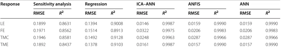
Table 8 Comparison of integrating artificial neural network and imperialist competitive algorithm (ICA–ANN) and ANFIS and regression and ANN and sensitivity analysis models
Response Sensitivity analysis Regression ICA–ANN ANFIS ANN
RMSE R2 RMSE R2 RMSE R2 RMSE R2 RMSE R2
LE 0.1899 0.8631 0.1394 0.9008 0.0146 0.9987 0.0159 0.9990 0.0159 0.9990
FE 0.1971 0.8562 0.1514 0.8913 0.0322 0.9975 0.0206 0.9983 0.0206 0.9983
TMC 0.1946 0.8581 0.1492 0.9128 0.0248 0.9963 0.0287 0.9966 0.0287 0.9966
(R2). Their results elucidated that hybrid ICA–ANN succeeded to denote lower modeling error than other methods [15]. In another study, Marto et al. applied ICA–ANN for prediction of flyrock induced by blasting and parameters of 113 blasting operations were accu-rately recorded. The results were clearly illustrated the superiority of the proposed ICA–ANN model in com-parison with the proposed BP-ANN model and empiri-cal approaches [31]. Nikoo et al. used ICA–ANN to predict the flood-routing problem. The results proved that using this technique on flood-routing problem is
a valid approach, which is not only simple but also reli-able [33].
Discussion
Comparison of models
models provide better results with regards to higher R2 values and lower RMSE values.
As it can be seen, moisture content, swelling index, soil compressibility factor and type of soil have low effect on cost and energy consumption. On the other hand, in case of specific gravity, when specific gravity of
of laborers increase as well and again more fuel will be consumed.
As it is clear, moisture content, swelling factor and type of soil, although less than other factors, have effects on energy consumption. Moisture content, soil compressibility factor and specific gravity in finetex-tured soils, like clays, and in soils with high organic materials lead to higher resistance against machine movement, which in turn adversely affect the energy consumption
Conclusion
Since a limited number of research related to energy consumption in land leveling has been done to measure the effects of soil and land properties, at this research, energy and cost of land leveling as a function of land characteristics have been evaluated. Studied character-istics of land in this research were: soil cut/fill volume, soil compressibility factor, specific gravity, moisture content, slope, sand percent, and soil swelling index. Based on these characteristics, artificial intelligence and computational methods such as ANN, and ICA-– ANN were used to determine the energy characteris-tics, i.e., FE, LE, TMC, TME. At this study, the ability of ANN, ICA–ANN, sensitivity analysis, regression, and ANFIS as well as PSO–ANN, GWO and SPSS for prediction of environmental indicators (LE, FE, TMC, and TME) during land leveling were investigated and compared. According to the results, 10-8-3-1, 10-8-2-5-1, 10-5-8-10-1, and 10-6-4-1 MLP network structures that were trained using Levenberg–Marquardt had the best performance. Sensitivity analysis revealed that only three variables including density, soil compress-ibility factor, and V had the highest effect on the out-put parameters including LE, FE, TMC and TME, and the accurate modes that relate each parameter to one another were extracted. Using regression method, only three variables including slope, V and SSI were deter-mined to be effective on FE. Results approved the supe-riority of integrated methods, especially ICA–ANN, compared to other methods such as regression and sta-tistical software such as SPSS and Minitab. Moreover, the ANFIS models with hybrid optimization method and Sugeno FIS type show better performance than the models based on back propagation and Mamdani tech-niques. All ANFIS-based models have R2 values above 0.995 and MSE values below 0.002.
Based on the results, ANN and ICA–ANN algorithms are the most capable methods to predict LE and FE. In the same way, GWO–ANN was found to be more pow-erful and accurate in prediction of TMC and TME. In fact, comparing ANN, ICA–ANN, PSO–ANN, GWO– ANN and sensitivity analysis methods in estimating the
amount of LE, FE, TMC and TME based on statisti-cal indicators shows that GWO–ANN and ICA–ANN methods are more accurate, despite very slight differ-ence between their results. On the other hand, sensi-tivity analysis method is the least accurate one. Ability of GWO–ANN and ICA–ANN models in prediction of sophisticated problems with high accuracy makes it a powerful tool for engineers and researchers to use it not only in agricultural operations, but also in other fields such as finance, mining, infrastructures, etc. Using this tool will lead to an economical land leveling operations in farm lands. These implications are consistent with the findings and conclusions of this study. Furthermore, implementing this technique on heavy operations such as land leveling will help in protecting the environment which in turn increases the life quality.
Abbreviations
GWO–ANN: Integrating Artificial Neural Network and Grey Wolf Optimizer (GWO); ICA–ANN: Integrating Artificial Neural Network and imperialist competitive algorithm; ANN: Artificial Neural Network; LE: environmental indicators: labor energy; FE: environmental indicators: fuel energy; TMC: total machinery cost; TME: environmental indicators: total machinery energy.
Authors’ contributions
IA carried out all studies about the work and cultivated the data which were necessary to be analyzed. FM participated in land leveling studies results acquisition. SA helped in design and studying of artificial neural networks ANFIS and statistical analyses. All authors read and approved the final manuscript.
Author details
1 Department of Surveying and Geometric Eng, Engineering Faculty, University
of Tehran, Tehran, Iran. 2 College of Agriculture, University of Basrah, Basrah,
Iraq. 3 College of Agriculture and Natural Resources, University of Tehran,
Tehran, Iran.
Acknowledgements
We are thankful to our colleagues, faculty and Ph.D. students who helped us at Department of Surveying and Geometrics Engineering, and Department of Agriculture and Natural Recourses of the University of Tehran, Iran, who provided expertise that greatly assisted the research.
Competing interests
The authors declare that they have no competing interests.
Availability of data and materials
The dataset supporting the conclusions of this article will not be shared due to performing our next projects with this software.
Consent for publication Not applicable.
Ethics approval and consent to participate Not applicable.
Funding
All parts of this research have been supported by the University of Tehran.
Publisher’s Note
Received: 20 January 2018 Accepted: 22 January 2019
References
1. Shakibai AR, Koochekzadeh S. Modeling and predicting agricultural energy consumption in Iran. Am-Eur J Agric. 2009;5(3):308–12. 2. Okasha EM, Abdelraouf RE, Abode MAA. Effect of land leveling and
water applied methods on yield and irrigation water use efficiency of maize (Zea mays L.) grown under clay soil conditions. World Appl Sci J. 2013;27(2):183–90.
3. Brye KR, Slaton NA, Norman RJ. Soil physical and biological proper-ties as affected by land leveling in a clayey aquent. Soil Sci Soc Am J. 2006;70(2):631–42.
4. McFarlane BL, Stump-Allen RCG, Watson DO. Public perceptions of natu-ral disturbance in Canada’s national parks: the case of the mountain pine beetle (Dendroctonus ponderosa Hopkins. Biolo Con. 2006;130(3):340–8. 5. Khan F, Khan SU, Sarir MS, Khattak RA. Effect of land leveling on some
physico-chemical properties of soil in district dir lower. Shar J Agric. 2007;23(1):108–14.
6. Severino G, et al. The IoT as a tool to combine the scheduling of the irrigation with the geostatistics of the soils. Fut Gen Computer Syst. 2018;82:268–73.
7. Moghaddam K, Far T. Laser land levelling as a strategy for environmental management: the case of Iran. Pollution. 2015;1(2):203–15.
8. Toro J, Requena I, Zambrano M. Environmental impact assessment in Colombia: critical analysis and proposals for improvement. Environ Impact Asses. 2010;30(4):247–61.
9. Giannino F, et al. A predictive decision support system (DSS) for a micro-algae production plant based on Internet of Things paradigm. Concurren Comput Prac Experience. 2018;30(15):e4476.
10. Diamantopoulou MJ. Artificial neural networks as an alternative tool in pine bark volume estimation. Comput Electron Agr. 2005;48:235–44. 11. Lei K, Qiu Y, He Y. A new adaptive well-chosen inertia weight strategy to
automatically harmonize global and local search ability in particle swarm optimization. In: Systems and Control in Aerospace and Astronautics 2006. 1st international symposium on systems and control in aerospace and astronautics. 2006. IEEE
12. Ahmadi MA, Ahmadi MR, Shadizadeh SR. Evolving artificial neural net-work and imperialist competitive algorithm for prediction permeability of the reservoir. Appl Soft Comput. 2013;13(2):1085–98.
13. Ahmadi MA, Soleimani R, Bahadori A. A computational intelligence scheme for prediction equilibrium water dew point of natural gas in TEG dehydration systems. Fuel. 2014;137:145–54
14. Ahmadi MA, Golshadi M. Neural network based swarm concept for prediction asphaltene precipitation due to natural depletion. J Petrol Sci Eng. 2012;98:40–9.
15. Taghavifar H, Mardani A, Taghavifar L. A hybridized artificial neural network and imperialist competitive algorithm optimization approach for prediction of soil compaction in soil bin facility. Measurement. 2013;46(8):2288–99.
16. Ahmadi MA, Bahadori A, Shadizadeh SR. A rigorous model to predict the amount of dissolved calcium carbonate concentration through-out oil field brines: side effect of pressure and temperature. Fuel. 2015;139:154–9.
17. Fereydooni M, Mansoori J. Evaluation of multilayer perceptron models and adaptive neuro-fuzzy interference systems in the simulation of groundwater level (case study: lamer plain. Indian J Fundam Appl life Sci. 2015;5:1076–83.
18. Fereydooni M, Mansoori B. Simulation depth of bridge pier scouring using artificial neural network and adaptive neuro-fuzzy inference sys-tem. Indian J Fund Appl Life Sci. 2015;5:2091–5.
19. Nazari-Shirkouhi S, Eivazy H, Ghodsi R, Rezaie K, Atashpaz-Gargari E. Solv-ing the integrated product mix-outsourcSolv-ing problem usSolv-ing the imperial-ist competitive algorithm. Expert Syst Appl. 2010;37(12):7615–26. 20. Atashpaz-Gargari, E. and C. Lucas. Imperialist competitive algorithm:
an algorithm foroptimization inspired by imperialistic competition. In: Evolutionary computation. CEC2007. IEEE Congress on; 2007. IEEE.
21. Abdechiri M, Faez K, Bahrami H. Adaptive Imperialist competitive algorithm (AICA). In: cognitive informatics (ICCI). 9th IEEE international conference. 2010. p. 940–945.
22. Ebrahimzadeh A, Addeh J, Rahmani Z. Control Chart Pattern Rec-ognition Using K-MICA Clustering and Neural Networks. ISA Trans. 2012;51(1):111–9.
23. Rajabioun R, Atashpaz-Gargari E, Lucas C. Colonial competitive algorithm as a tool for nash equilibrium point achievement. In: International Confer-ence on Computational SciConfer-ence andIts Applications. Springer; 2008. 24. Abdi B, Mozafari H, Ayob A, Kohandel R. Imperialist competitive algorithm
and its application in optimization of laminated composite structures. Eur J ScI R. 2011;55(2):174–87.
25. Talatahari S, Kavehand A, Sheikholeslami R. Chaotic imperialist competi-tive algorithm for optimum design of truss structures. Str Multidiscip Optim. 2012;46(3):355–67.
26. Kaveh A, Talatahari S. Optimum design of skeletal structures using imperi-alist competitive algorithm. Comput Struct. 2010;88(21–22):1220–9. 27. Mohammadi A, Rafiee S, Keyhani A, Emam-Djomeh Z. Modelling of
kiwifruit (cv.Hayward) slices drying using artificial neural network. In: 4th international conference on energy efficiency and agricultural engineer-ing. Bulgaria: Rousse; 2009. p. 397–404.
28. Movagharnejad K, Nikzad M. Modeling of tomato drying using artificial neural network. Comput Electron Agr. 2007;59(1):78–85.
29. Cassel D, Wood M, Bunge RP, Classer L. Mitogenicity of brain axolemma membranes and soluble factors for dorsal root ganglion schwann cells. J Cell Biochem. 1982;18(4):433–45.
30. Tiryaki B. Predicting intact rock strength for mechanical excavation using multivariate statistics, artificial neural networks, and regression trees. Eng Geol. 2008;99(1–2):51–60.
31. Marto A, Hajihassani M, Armaghani D, Mohamad ED, Makhtar AM. A novel approach for blast-induced flyrock prediction based on imperial-ist competitive algorithm and artificial neural network. Sci World J. 2014;2014(15):1–11.
32. Azadeh A, Ghaderi SF, Sohrabkhani S. Annual electricity consumption forecasting by neural network in high energy consuming industrial sec-tors. Energy Convers Manage. 2008;49(8):2272–8.