http://www.sciencepublishinggroup.com/j/ijass doi: 10.11648/j.ijass.20190702.11
ISSN: 2376-7014 (Print); ISSN: 2376-7022 (Online)
Interstellar Medium Parameters in Front of the External
Bow Shock
Pavel Alexandrovich Sedykh
Department of Physics, Irkutsk National Research Technical University, Irkutsk, Russian Federation
Email address:
To cite this article:
Pavel Alexandrovich Sedykh. Interstellar Medium Parameters in Front of the External Bow Shock. International Journal of Astrophysics and Space Science. Vol. 7, No. 2, 2019, pp. 21-26. doi: 10.11648/j.ijass.20190702.11
Received: July 15, 2019; Accepted: August 13, 2019; Published: August 26, 2019
Abstract:
We know that it is the front of the Earth’s bow shock where the solar wind kinetic energy flux is transformed into the other kinds the most intensively. In our previous studies, we obtained important relationships that enable calculating the key parameters at transition through the Earth’s bow shock front. One of the most important sources of information on physical processes at the heliosphere boundary are the Voyager 1 and 2 spacecrafts. Since both the solar wind and interstellar medium are supersonic streams, two shocks are formed when flowing around the heliopause. The internal shock, in which the solar wind decelerates to subsonic velocity, is called the heliospheric shock. In the external bow shock, the interstellar gas supersonic flux is decelerated. The aim of this paper is to generalize the previously obtained equations to the processes in the external bow shock region. If Voyager-1 was equipped with a greater set of measuring instruments, we could have already provided estimations of the interstellar medium key parameters, and described in physical terms what this medium is, using relationships and equations from our studies.Keywords:
External Bow Shock, Interstellar Medium, Set of Measuring Instruments, Computing of Parameters1. Introduction
The bow shock (BS) front is the main converter of the solar wind kinetic energy into the electromagnetic energy [8, 10]. At transition through the front, the intensity of the tangential component of the solar wind magnetic field and density grow several times. Therefore, among other things, the BS front is a current layer. Since the magnetic field plasma passes through the front, there arises an electrical field in the front coordinate system [11]. Thus, the BS front is the source of electrical power [11]. This electrical power is sheared by two sinks (consumers) – the transition layer (TL or magnetosheath) and the magnetosphere. We know the relationships between the magnetic field values ahead and behind the BS. They allow calculating the current on the BS front. According to [8, 10], this electric current value depends on the normal component's jump, and the electric current direction depends on the direction of magnetic field ahead the BS. This current is considerably divergent, i.e. it must close somewhere behind the BS front. This closure may occur in the magnetosphere or in the transition layer. Let's briefly address the origin of the external electric current. The
to calculate key parameters and to model the processes in the bow shock region.
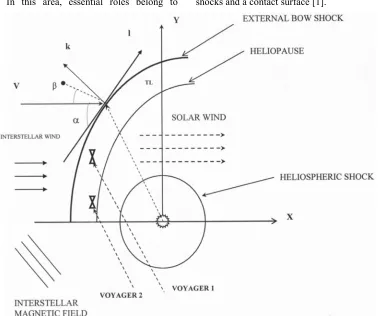
The interstellar medium and solar wind interacting; a complex structure called the heliosphere shock layer is formed (see Figure 1). The heliosphere shock layer is multicomponent. In this area, essential roles belong to
protons and electrons of the solar wind and interstellar medium, trapped ions, interstellar hydrogen atoms, heliosphere and interstellar magnetic fields, and galactic and anomalous cosmic rays components. In the concept accepted at the moment, the shock layer structure is described by two shocks and a contact surface [1].
Figure 1. A sketch of the external bow shock, of the Transition Layer (TL), heliopause.
The location of the orthogonal coordinate system (X, Y) with the origin in the Sun’s center and the location of the local coordinate system (l, k, n); axis l is directed along the tangent to the external bow shock front, axis k is directed perpendicularly to the tangent (to the external bow shock front) and axis n is directed perpendicularly to the sketch plane (i.e. the n- axis supplements this system to the right one). α - is an angle between the tangent to the external bow shock front and axis X; β - is an angle between the interstellar wind velocity and projection of interstellar magnetic field onto the equatorial plane B1eq.
We shall note that according to some papers, in the presence of interstellar magnetic field strong enough, there might be no external bow shock, since the Mach-Alfven number in the interstellar medium is less than 1. In case of partially-ionized interstellar medium, neutral atoms interact with the disturbed plasma component by recharging. The recharge process leads to formation of a so-called "hydrogen wall" – region in front of the heliopause proximal to the interstellar medium with increased concentration of interstellar atoms. The hydrogen wall is composed of secondary atoms formed resulting from recharging of primary interstellar atoms on decelerated interstellar protons.
One of the most important sources of information on physical processes at the heliosphere boundary are the Voyager 1 and 2 spacecrafts. As early as in 2011-2013, new unique data about heliosphere boundary from the Voyager-1, 2 spacecrafts became available. Starting from spring 2011, the Voyager-1 spacecraft has been recording a practically zero speed of the solar wind and during some periods its radial velocity was negative [4]. In August 2012, Voyager-1 revealed a dramatic reduction in fluxes of anomalous cosmic rays component, and a simultaneous increase of cosmic rays galactic component fluxes and increased value of magnetic field induction from ~ 0.2 nT to ~ 0.4 - 0.5 nT [3, 4]. However, the magnetic field vector direction has not changed, coinciding with the direction of heliospheric magnetic field. In April-May 2013, the PWS instrument has detected 2.6 kHz radiation. Analysis of this radiation enabled scientists to get a rough estimate of electron density at the generation point of this radiation, which is ~ 0.08 cm-3, this exceeds considerably the solar wind density. The analysis of the gradient the frequency varies with, depending on distance, led to the conclusion that Voyager-1 crossed the heliopause on August 25, 2012 [3].
the local interstellar medium indicate that the speed of the interstellar wind is most likely less than both the fast magnetosonic speed and the Alfven speed (but greater than the slow magnetosonic speed). In the study [14] the authors found that the bow shock would take a different form, what is known as a “slow bow shock”. The authors say that the Voyager 1 probe is expected to pass through the bow shock well after it leaves the heliosphere, although by then, its battery will be long dead [14].
In the paper [2] is noted that the Voyager 1 spacecraft is currently in the vicinity of the heliopause, which separates the heliosphere from the local interstellar medium. There has been a precipitous decrease in particles accelerated in the heliosphere and a substantial increase in galactic cosmic rays.
The authors devised a test to determine whether or not Voyager 1 has left the heliosphere. Previously, researchers found that Voyager 1 has encountered increased density of electron plasma, which they interpret as evidence that Voyager 1 is in interstellar space. According to [2] if Voyager 1 encounters another current sheet, it will provide strong observational evidence that the heliopause has not yet been crossed. Using data about Voyager 1’s current location and speed and the dynamics of the Sun’s current sheets, the authors determined that the spacecraft should encounter another current sheet during 2015 and certainly by no later than the end of 2016[2].
It should be noted that interstellar neutrals have been observed by IBEX for He [5] and O [7], which are used to determine the plasma flow in the outer heliosheath and by inference interstellar plasma conditions, which we want to measure in-situ and use to deduce the interstellar conditions. Kubiak et al. [5] analyzed the IBEX observations of neutral He (following the high-precision determination of the temperature and velocity of the pristine interstellar neutral (ISN) He). Kubiak et al. [5] used the same simulation model and a parameter fitting method very similar to that used for the analysis of ISN He (during the observation seasons 2010–2014 and covering the region in the Earth’s orbit where the Warm Breeze (WB) persists). Kubiak et al. [5] approximated the parent population of the WB in front of the heliosphere with a homogeneous Maxwell–Boltzmann distribution function and found a temperature of ~9500 K, an inflow speed of 11.3 km⋅ s−1. According to [5] the abundance of the WB relative to ISN He is 5.7% and the Mach number is 1.97. The newly determined inflow direction of the WB, the inflow directions of ISN H and ISN He, and the direction to the center of the IBEX Ribbon are almost perfectly co-planar, and this plane coincides within relatively narrow statistical uncertainties with the plane fitted only to the inflow directions of ISN He, ISN H, and the WB. This co-planarity lends support to the hypothesis that the WB is the secondary population of ISN He and that the center of the Ribbon coincides with the direction of the local interstellar magnetic field [5].
Park et al. [7] investigated (using the observations of IBEX-Lo He and O) the directional distributions of the
secondary interstellar neutral (ISN) populations (He and O) at the region of Earth’s orbit. According to [7] the secondary populations are created by charge exchange between ISN atoms and interstellar ions in the outer heliosheath. Their results indicated that the secondary populations have lower bulk speeds relative to the Sun and their flow directions deviate from the primary gas flow. These results [7] may indicate that one side of the outer heliosheath is thicker than the other side relative to the flow direction of the primary interstellar gas flow.
Zirnstein et al. [15] investigated the characteristics and geometry of the inner heliosheath (IHS) plasma and their impact on the heliotail structure. Zirnstein et al. [15] analyzed the key parameters and processes that form and shape the port and starboard lobes, which are distinctly different from the north and south lobes.
The main purpose of the paper is to study physical processes at the heliosphere boundary (the region of the solar wind interaction with the interstellar medium) by means of theoretical analysis of some experimental data. With the Voyagers and IBEX returning many new puzzles, this paper could be interesting because it might address in a complementary way questions that are hotly debated in the heliophysics community.
2. Some Application of the Derived
Equations for the External Bow Shock
Baranov et al. [1] proposed a structure with two shocks, which is now the basis of a concept of the heliosphere shock layer (Figure 1). Heliopause, which is a tangential discontinuity surface, separates the interstellar medium charged component from the plasma of the solar wind. Because both the solar wind and interstellar medium are supersonic streams, two shocks are formed when flowing around the heliopause: heliospheric shock and external bow shock.
equilibrium. The local interstellar medium also contains neutral atoms, which interact with the solar wind plasma through charge exchange, electron impact ionization or photoionization. Due to all these complications, one could apply the classical Rankine-Hugoniot relations only with combinations of equations from our studies; and one should take into account the results of recent computer simulations.
Let's also address other key parameters. We can choose the system of coordinates as a base beginning at the center of the Sun (Figure 1). I shall use local coordinate system (l, k, n). I will follow our previously published papers [8, 9, 11] in the approach to the external bow shock description.
I assume a spherically symmetric heliospheric bow shock like for the Earth, while there is hypothesis, since the Voyager passages of the termination shock and through IBEX observations, that the heliosphere might be strongly distorted. I need to make such simplification to solve the problem analytically.
The correspondences of the parameters in front of and behind (in TL) the external bow shock will be the following. The plasma density is defined as:
2 1 1 ; ; 1
γ
ρ
ρ δ δ
γ
+ = ⋅ = −One can derive the gas pressure:
( )
2 2
2 1 1
sin 2
1 g
p ρV α
γ =
+
The tangential velocity component will be:
( )
2l 1l 1cos V =V =V α
The normal velocity component will be:
( )
1 2 1 sin k k VV V α
δ δ
= =
The vertical component of the magnetic field will be:
2n 1n B =B ⋅δ
The tangential component of the magnetic field is defined as:
(
)
2l 1l 1eq cos
B =B ⋅ =
δ
B ⋅δ
α β
+The normal component of the magnetic field is defined as:
(
)
2k 1k 1eqsin
B =B =B
α β
+In these equations, numbers 1, 2 correspond to the interstellar medium and the transition layer, respectively; γ – is the adiabatic exponent; α – is the angle between the tangent to the external bow shock front and the X-axis; β – is the angle between the direction of the interstellar wind velocity and the projection of the magnetic field onto the equatorial plane B1eq (see Figure 1).
Besides, knowing numerical values of parameters in the equations, we can set various values of γ. Thus, one can obtain the additional information on properties of medium.
We should note that owing to final curvature of the external bow shock front surface there appears a force (additional) of magnetic tension: Fn = (B∇)Bn/4π. This force must be put in equilibrium by additional Ampere force: j*τBl/c; here j*τ is density of additional current: j*τ=c⋅(∂Βn/∂l)/4π. We can find the density of the basic current jτ: jτ= c (δ - 1)B0l/d, where d is front thickness. Since d <<Xh, Xh - is the distance from the origin of system of coordinates to the shock front, then additional electric current is much less than basic one. The effect of curvature should not be taken into account, at least until δ notably differs from 1. We can obtain the equation for the gradient of plasma pressure and the inertial force behind the external bow shock front (i.e. in the transitional layer):
2 2 2 1 1 sin2
1
g
dP V d dl dl ρ α γ = + ;
(
)
2 2 21 1 2
2 2 1 sin
2 V dV d dl dl ρ δ ρ α δ −
= − ; (1)
whereδ =(γ+1)⁄(γ-1).
Thus, substituting these expressions into the equation for current density, we can obtain:
2 2
2 2
g
c V
j B p
B ρ ∇ = × ∇ + ; 2
2 2 2
2 2
2
g l n
k
dP dV B
j c
dl ρ dl B
= +
;
or
( )
1 2 22 2 2 1 1
2 2 sin 1 n k B d
j c V
dl
B
δρ
α
γ
= −− , (2)
where j2k – is an electric current, which flows across the transition layer;
(
) (
)
(
)
2 2 2 2 2 2
2 1n 1eq 1 2 1 sin cos B =B δ +B δ + − δ − α⋅ α ; (3)
The surface density of the current, flowing in the transitive layer along it, will be the integral from jl across the layer from heliopause up to the external bow shock:
( )
1 2 2 ( ) g g l nP bs P h J cB
B
δ −
= ; in this expression Pg(bs) and
Pg(h) are gas pressure under the external bow shock and on the heliopause, respectively.
One can obtain the important relationship for the physics of the shock layer, in which the hydrodynamic and electrodynamic quantities are in the left and right sides of this equation, respectively:
(
)
e i i
e g i g i e
dV
V P V P Ej V V
dt ρ
∇ + ∇ = − − ,
where e – index for electrons; i – index for ions.
We can also assume, that the front form of the external bow shock is given, as well as the form of heliopause. Heliopause may be well approximated by biaxial hyperboloid. One can assume that both heliopause and external bow shock are paraboloids of rotation and differ only in various distances to the nose point. Such step is connected with the fact that the form of heliopause and especially forms of the external bow shock front differ little from paraboloids of rotation, at the same time all analytical expressions drastically become simpler (see corresponding equations in [6]). Parabola is some compromise between ellipsoid (closed model) and hyperboloid (open model). Further, we can apply important relationships from our papers that enable calculating the key parameters at transition through the external bow shock front.
The system ‘external bow shock-TL-heliopause-heliospheric shock’ is unique plasma laboratory. Thus, if we knew such parameters e.g. as plasma density, plasma pressure, gas pressure gradient, components of magnetic field, electric field, fluxes of particles in the transition layer, we would be able to determine key parameters in front of the external bow shock.
3. Conclusion
To obtain the analytically solution of the problem, we have been compelled to make some simplifications (by analyzing a maximum possible simple model that at the same time retains the most important traits of reality). In most cases, we followed [1] in the approach to the heliosphere shock layer description. In this paper, we use the results of previous studies, in which the following was obtained: the expressions for the magnetic field components at transition through the Earth’s bow shock front; the equations for plasma density; the expressions for electrical current generated in the bow shock front and closed through the Earth’s magnetosphere, and for the magnetopause potential as a function of the solar wind parameters – plasma density, velocity and intensity of the interplanetary magnetic field (IMF); and also, the expressions for the transition layer basic parameters as functions of the IMF components etc.
We can use the obtained important expressions and relationships to determine the interstellar medium parameters. It is known that the Voyager-1 spacecraft was equipped with the following scientific instruments: UV spectrometer, interference IR spectrometer, photopolarimeter, low-energy charged particle detector, instrument to determine radio waves of planets, instrument to determine waves in plasma, magnetometer to measure weak magnetic fields, magnetometer to measure strong magnetic fields, cosmic ray detector, and plasma detector.
If Voyager-1 was equipped with a broader range of measuring instruments, we could have already provided estimations of the interstellar medium key parameters, using the above mentioned relationships, equations. In other words, if we knew the parameters in the transition layer, we would be able to calculate them ahead the external bow shock front.
Thus, we could have now made preliminary conclusions on the behind-the-heliosphere medium, i.e. in the interstellar space. It should be noted that even if the Voyager-1,2 spacecrafts were initially equipped with a great set of measuring instruments, they would need to be protected against cosmic radiation. Otherwise, cosmic ionizing radiation would destroy almost all the electronics inside the apparatus on their way out of the solar system.
I have provided the specific equations. We have all the essential equations to calculate the parameters; we have a developed mathematical apparatus to convert the relevant physical values at transition through the bow shock front, a set of computer programs with the user interface; two spacecrafts are in the appropriate region, but they do not have the necessary measuring instruments. This essential set of measuring instruments that would enable us to obtain a series of numerical estimates of key parameters can be presented as follows:
(1). Magnetometer. FluxGate Magnetometer (Magnetic Field Vector, spin resolution; Magnetic Field Magnitude).
(2). Ion and electron sensor combination that operates in the bulk plasma energy regime/Instrument to measure plasma density and composition (Electron, Proton, and Alpha-particle Monitor).
(3). Electron Diagonalized Temperature. Electron Symmetry Vector. Ion Diagonalized Temperature. Ion Symmetry Vector.
(4). Electrostatic Analyzer.
(5). Electric Field Variation, based on spin plane component.
We should note that to date, this set of measuring instruments is not a hard-to-obtain one, it is readily available on research satellites. There is bound to be a huge time-lag before Voyager spacecrafts can travel through the interstellar space medium, and we could already be able to learn this medium properties, because the parameters behind the shock front are well-determined by the known laws and relationships. Parameters of the medium behind the front of the external bow shock contain much information about physical parameters ahead of the external bow shock front (about interstellar medium). Any follow-up mission to the heliospheric boundary that would be worth the effort and that a space agency would be willing to fund, which could carry this instrumentation, almost for sure would be an interstellar probe that continues into the interstellar medium proper. This would make most of the motivation for similar studies.
The proposed study would significantly reduce the current uncertainties concerned with the structure of the heliosphere shock layer behind the external bow shock, and with measuring the parameters of the local interstellar medium that surrounds the solar system.
Acknowledgements
The research of this paper was funded by the programs of Irkutsk National Research Technical University.
[SYSTEMATIC REVIEW or META-ANALYSIS] are from previously reported studies, which have been cited.
Conflict of Interest
The author declares that there is no conflict of interest regarding the publication of this paper.
References
[1] Baranov V. B., Krasnobayev K. V., Kulikovsky A. G., 1970. Model of the solar wind and interstellar medium interaction, Reports of Academy of Sciences. USSR, 1, 105.
[2] Gloeckler G. and Fisk L. A., 2014. A test for whether or not Voyager 1 has crossed the heliopause. Geophysical Research Letters, doi: 10.1002/2014GL060781, 41, 15.
[3] Gurnett D. A., Kurth W. S., Burlaga L. F., Ness N. F., 2013. In Situ Observations of Interstellar Plasma with Voyager 1. Science. 1241681, doi: 10.1126/science.1241681.
[4] Krimigis S. M., Roelof E. C., Decker R. B., Hill M. E., 2011. Zero outward flow velocity for plasma in a heliosheath transition layer. Nature, 474, p. 359–361.
[5] Kubiak Marzena A., et al. 2016. Interstellar neutral helium in the heliosphere from IBEX observations. iv. Flow vector, mach number, and abundance of the warm breeze. The Astrophysical Journal Supplement Series, 223: 25. doi: 10.3847/0067-0049/223/2/25.
[6] Madelung, E., 1957. Die mathematischen hilfsmittel des physikers. Berlin. Gottingen. Heidelberg. Springer-Verlag. p. 500.
[7] Park J., Harald Kucharek, Eberhard Möbius, André Galli,
Marzena A. Kubiak, Maciej Bzowski, and David J. McComas. 2016. IBEX observations of secondary interstellar helium and oxygen distributions. The Astrophysical Journal, 833: 130. doi: 10.3847/1538-4357/833/2/130
[8] Ponomarev E. A., Sedykh P. A., Urbanovich V. D., 2006. Bow shock as a power source for magnetospheric processes. Journal of Atmospheric and Solar-Terrestrial Physics, 68, p. 685–690.
[9] Sedykh P. A., 2011. On the role of the bow shock in power of magnetospheric disturbances. Sun & Geosphere. Special issue of ISWI /United Nations/NASA/JAXA/AGU/ESA/; ISSN 1819-0839. 6 (1), P.27-31.
[10] Sedykh P. A., E. A. Ponomarev., 2012. A structurally adequate model of the geomagnetosphere. Stud. Geophys. Geod., AS CR, 56, doi: 10.1007/s11200-011-9027-3, p. 110–126. [11] Sedykh P. A., 2014. Bow shock. Advances in Space Research,
Elsevier Science., JASR11746.
[12] Sedykh P. A. 2015. Bow shock: Power aspects. Nova Science Publ. NY USA, in Horizons in World Physics. 285. p. 23-73. [13] Whang, Y. C., 1987. Slow shocks and their transition to fast
shocks in the inner solar wind. J. of Geophys. Res., V. 92, 5. p. 4349–4356.
[14] Zieger, B., M., Opher, N. A., Schwadron, D. J. McComas, and G. Tуth., 2013. A slow bow shock ahead of the heliosphere. Geophysical research letters, v. 40, p. 2923–2928, doi: 10.1002/grl.50576.