www.j-sens-sens-syst.net/5/337/2016/ doi:10.5194/jsss-5-337-2016
© Author(s) 2016. CC Attribution 3.0 License.
Sensor defect detection in multisensor
information fusion
Jan-Friedrich Ehlenbröker, Uwe Mönks, and Volker Lohweg inIT – Institute Industrial IT, Langenbruch 6, 32657 Lemgo, Germany
Correspondence to:Jan-Friedrich Ehlenbröker ([email protected])
Received: 15 October 2015 – Revised: 25 June – Accepted: 26 July 2016 – Published: 18 October 2016
Abstract. In industrial processes a vast variety of different sensors is increasingly used to measure and control
processes, machines, and logistics. One way to handle the resulting large amount of data created by hundreds or even thousands of different sensors in an application is to employ information fusion systems. Information fusion systems, e.g. for condition monitoring, combine different sources of information, like sensors, to generate the state of a complex system. The result of such an information fusion process is regarded as a health indicator of a complex system. Therefore, information fusion approaches are applied to, e.g., automatically inform one about a reduction in production quality, or detect possibly dangerous situations. Considering the importance of sensors in the previously described information fusion systems and in industrial processes in general, a defective sensor has several negative consequences. It may lead to machine failure, e.g. when wear and tear of a machine is not detected sufficiently in advance. In this contribution we present a method to detect faulty sensors by computing the consistency between sensor values. The proposed sensor defect detection algorithm exemplarily utilises the structure of a multilayered group-based sensor fusion algorithm. Defect detection results of the proposed method for different test cases and the method’s capability to detect a number of typical sensor defects are shown.
1 Introduction
A sensor, which is acquiring signals in an application, is gen-erally assumed to be operating correctly. Sensors can never-theless fail and do so during typical operation. Failure causes include improper handling, wear and tear, or random failure. The failure may on the one hand be a complete failure of the sensor, which is easily detectable, as the sensor stops deliv-ering any data. On the other hand, partial defects are more difficult to detect: if a sensor continuously delivers values, it is neither directly detectable, nor decidable if the sensor mea-surements are valid or not. In case of partial defect, the sensor might produce values that deviate more from the true value than their given accuracy. This is problematic for condition monitoring purposes in manufacturing processes. Here, sen-sor defects lead to a decrease in product quality or a reduc-tion in the produced quantity of a given product. Depending on the sensor’s use case, a sensor defect has possibly even more severe consequences.
There are multiple possible ways to detect and handle sen-sor defects. An overview over the most important methods for detecting sensor faults is given in the following.
Simple approaches use rule-based threshold systems to de-tect sensor faults. For example in Sharma et al. (2010) the standard deviation of a sensor measurement within a win-dow is used to detect sensor noise and the rate of change of a sensor measurement to detect short peak errors.
Apart from the aforementioned simple approaches, most algorithms are more complex and use statistical measures, machine learning methods or a combination of both.
dimensional-ity that allows for a linear separation between the different fault states and the non-faulty state. More complex PCA-based methods use dynamic PCA-PCA-based approaches for sen-sor fault detection, as for example in Hu et al. (2012), where a self-adapting PCA-based method is used. For the detection of sensor defects in non-linear systems, PCA-based methods that use kernel functions are proposed (Choi et al., 2005).
Bayesian belief network (BBN) based methods are pro-posed in Mehranbod et al. (2003, 2005). They model every sensor as its own multiple-node BBN. Training data are used to generate state probabilities (example states: very nega-tive, neganega-tive, zero, posinega-tive, very positive) for the nodes and when there are deviations from these trained state probabili-ties a sensor error is detected.
Artificial neural networks (ANNs) (cf. e.g. Mattern et al., 1998; Xu et al., 1999; Zhu et al., 2012; Helwig et al., 2015) and approaches based onclustering(cf. e.g. Bay and Schwabacher, 2003; Kusiak and Song, 2009) to detect sensor faults. While clustering-based algorithms detect sensor faults with the help of outlier detection, ANNs are used to gener-ate a fault-free sensor output via sensor correlation (Mattern et al., 1998; Xu et al., 1999) or to detect if the sensor state is faulty or fault free (Zhu et al., 2012).
One approach is the application of sensors that execute self-tests to detect the sensor performance and sensor de-fects. Depending on the type of sensor and the intended use, this may be a valid way to handle sensor defects. Never-theless, self-testing capabilities are often limited to simple function tests. Additionally, such sensors have higher acqui-sition costs compared to sensors without self-test abilities: considering standard off-the-shelf sensors, additional elec-tronics must be integrated to each sensor to facilitate self-testing. This requires additional engineering, hardware, and production costs, which are added on top of the original sen-sor price. Moreover, sensen-sors with self-test abilities are not available for every use case, especially when applications im-pose special requirements, e.g. explosion protection.
The approach followed in this contribution is the appli-cation of multiple sensors for monitoring one and the same object or property. In such a use case, standard sensors can be applied with no additional acquisition costs. Their signals are collected, aggregated, and processed in a multisensor infor-mation fusion process. The fusion system serves for super-vision of the monitored system and also of the applied sen-sors. Here, additional one-time costs for the engineering and acquisition of the fusion system apply instead of increased costs for each sensor. In addition, retrofitting of existing ap-plications is facilitated in this way. Then already applied sen-sors are utilised for fusion, which is enriched by defect de-tection. The fundamentals of such a multisensor information fusion approach are described in the following section.
Decision unit
Decision
Classification
Feature
Feature extraction units
Raw data
Classification units
Sensor units
Sensors/measurement modules
Physical device/environment
Feature
database . . .
. . .
. . .
Figure 1.Multimodal system.
1.1 Multisensor information fusion
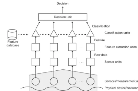
Many recent systems are based on one main sensory appa-ratus. They rely on the evidence of a single source of in-formation (e.g. photodiode scanners in vending machines, greyscale cameras in inspection systems). These systems, calledunimodal systems, have to contend with a variety of general difficulties. According to Ross and Jain (2005), these are raw data noise, intraclass variations, interclass similari-ties, and non-universality. Some of these mentioned limita-tions are overcome by the inclusion of multiple information sources. Such systems, known as multimodal systems, are expected to be more reliable due to the presence of multiple, partly signal-decorrelated, sensors. They address the prob-lems of non-universality and, in combination with meaning-ful interconnection of signals (fusion), the problem of inter-class similarities. At least, they can inform the user about problems with intraclass variations and noise. A generic mul-timodal system consists of four important units (cf. Fig. 1): (i) the sensor unit, which captures raw data from different measurement modules (i.e. sensors); (ii) the feature extrac-tion unit, which extracts an appropriate feature set as a rep-resentation for the system, from which the raw data are cap-tured; (iii) the classification unit, which compares the current features to their corresponding features stored in a database; (iv) the decision unit, which uses the classification results to determine whether the obtained results represent, e.g., a safe state of a hazardous material store (Lohweg and Mönks, 2010b).
The basic information fusion concept relies on the fact that the lack of information supplied by sensors is completed by the fusion process. It is assumed that, for example, two sen-sors (S1andS2) with different active physical principles (e.g.
infor-mation, which is more dense and of higher quality than every single data source (Luo and Kay, 1989) and thus a decrease of the result’s inherent uncertainty.
A simple way to process multiple observations in an in-formation fusion sense is a threshold system. Every sensor observation is classified individually, based on a threshold. These results are fed into a majority voting system to gener-ate a global decision about a status (Alpaydın, 2010). This approach may decrease the impact of a sensor defect, as multiple non-defective sensors overrule one defective sensor. Nevertheless, such systems are too simple to model a com-plex application sufficiently. Hence, more adequate (but also more complex) multisensor information fusion algorithms are used for the processing of sensor observations and the robust determination of a system’s state. These methods are known in the literature for many years (Khaleghi et al., 2011; Hall and Llinas, 2001a). This field has gained increasing at-tention starting in the 1970s when new sensors, advanced processing techniques, and increasingly powerful processing hardware became available. Starting then, appropriate data processing models and fusion algorithms have been driven nearly exclusively by applications in the military defence sector. During the 1990s and early 2000s, those algorithms have been adopted by the civil sector for applications in in-dustrial fault diagnosis and condition monitoring applica-tions (Hall and Llinas, 2001a). A current fusion definition was introduced by Steinberg and Bowman (2001):
Definition 1. Information fusion (Steinberg and Bowman, 2001, p. 2–4): “[the] process of combining data or in-formation to estimate or predict entity states.”
Fusion is possible at three distinct levels (Hall and Lli-nas, 2001b). Atsignal level, sensor signals are combined. It is necessary that the signals are comparable in the sense of data amount, i.e. sampling rate (adaption), dimension, reg-istration, and time synchronisation. If this constraint cannot be fulfilled, fusion on any of the following two levels is ap-propriate. At feature level, signal descriptors (features) are combined. Human cognitive functions rely on this associa-tion principle for recogniassocia-tion tasks. Atsymbol level, classifi-cation results are combined. This happens either after obtain-ing all individual decisions per sensor, or on top of a number of features or signal level fusion steps. The degree of ab-straction increases from signal level to symbol level, whereas the fusion itself is more efficient with increasing abstraction. Nevertheless, additional processing steps in advance to fu-sion might increase the overall complexity.
Besides, Ross and Jain (2005) state that fusion at an early processing stage is usually more effective than at a later stage, since input signals or features contain more informa-tion about the physical data than score value outputs of clas-sifiers. High abstraction level fusion is less effective also due to the fact that data reduction methods are applied in the in-termediate steps resulting in information loss (cf. Hall and Llinas, 2001b).
1.2 Related work
New concepts of distributed intelligent sensors have recently been introduced, in which an intelligent sensor is defined to be a system equipped with communication and process-ing capabilities, and acquires data from several elementary sensors attached to it (Duquet, 2015). Such concepts and ar-chitectures pose challenges to the design and operation of distributed monitoring systems (Mönks et al., 2015), among which is the handling of conflicts between sensor observa-tions during operation: conflict occurs whenever information bear evidence for not only one opinion/proposition, but also for another. This might either be due to actual failure in the observed process or system, or caused by one or more de-fective sensors. The latter case is the most severe one, since wrong decisions might be derived if sensors were considered reliable, although they are not.
Conflict handling is to a certain extent independent from the model applied to represent the information: while prob-ability theory (Jaynes, 2003; Bishop, 2009) and possibil-ity theory(Zadeh, 1978; Dubois and Prade, 1993) need to incorporate further processing steps for conflict handling, the Dempster–Shafer theory of evidence (DST) (Dempster, 1967; Shafer, 1976) is inherently designed to handle con-flicts. Nevertheless, the DST has shown to bear defects with respect to high-conflicting situations (cf. e.g. Zadeh, 1986; Yager, 1987).
A conflict-handling data fusion algorithm, based on the DST and improving its deficiencies, is the multilayer attribute-based conflict-reducing observation (MACRO) sys-tem (Mönks and Lohweg, 2013, 2014). Its fusion algorithm has shown good performance, especially in situations, where the input data are conflicting (Mönks et al., 2012). It never-theless offers no direct way for the fusion algorithm to detect defective sensors. The situation is similar for other sensor fusion approaches like Bayes’ theorem in the scope of prob-ability theory (Bishop, 2009), Dempster’s rule of combina-tion in the scope of DST (Shafer, 1976), or ordered weighted averaging (OWA) aggregation (Yager, 1988) in the scope of fuzzy set theory (Zadeh, 1965). They are all standard and widely applied fusion approaches, which do not offer inher-ent defect detection methods.
(fail-ure, no failure). During sensor fusion, the state of a sensor is used to exclude sensors that have a failure state.
Another exception is Krüger (2015), where conflicts in Bayesian networks are used to detect sensor failures. In this work four approaches for sensor failure detection are de-scribed. Two of the described approaches are based on binary conflicts (conflict present or no conflict present), while the other two approaches utilise a gradual conflict measure that shows the actual level of conflict. For the approaches with bi-nary conflicts the frequency of conflicts is used as a measure for defect detection. The algorithms based on gradual con-flicts use the mean gradual conflict value for defect detection. The final defect detection is carried out with the help of de-tection thresholds. Furthermore, all approaches described in Krüger (2015) use an adjustable sliding test-window, which incorporates multiple classification cases for defect detec-tion.
Other sensor fusion approaches incorporate sensor relia-bility or similar values into the fusion process. In Elouedi et al. (2004) a DST-based sensor fusion approach that incor-porates a discounting factor for sensors is proposed. This dis-counting factor is computed based on the existing knowledge compared to the measurement of a sensor. The difference be-tween the known class of the objects in a training data set and the assessment of a sensor is used to determine the discount-ing factor, with higher differences resultdiscount-ing in a higher dis-counting factor. The smaller the disdis-counting factor, the more reliable the sensor considered.
The reliability computation method proposed by Martin et al. (2008) is also based on DST. It utilises the distances between a sensor’s measurement and the combination of all other sensors’ measurements to compute a conflict measure. The reliability value of a sensor is then in turn computed based on a decreasing function, which utilises the conflict measure. This results in a lower reliability value for sensors with higher conflict, which is used as a discounting factor during the sensor fusion process.
The approach presented in this article is partly based on Glock et al. (2011), which introduces a method to determine the reliability of sensors. This is in turn used to weight the sensors during a sensor fusion process.
In summary, sensor fusion approaches are available, which incorporate a form of reliability computation for sensors. Their outcome is applied to weight sensors during the sen-sor fusion process (Elouedi et al., 2004; Martin et al., 2008; Glock et al., 2011). Only a few methods use sensor fusion approaches to actually detect sensor defects (Ricquebourg et al., 2008; Krüger, 2015).
This article proposes a method that uses group-based structures where the sensor defects are computed based on groups of sensors instead combining all sensors at once, as other approaches do.
1.3 Structure
In this paper, a method is proposed that utilises the inher-ent multilayer group-based structure of MACRO and detects sensor defects with the help of sensor consistency compu-tations. While the structure of MACRO is utilised in the presented approach, it is also applicable in other group-based fusion approaches. Its effectiveness is demonstrated in the scope of the research project “itsowl-IGel” (itsowl-IGel, 2015). The main goal of itsowl-IGel is the development of a condition monitoring and early warning system for haz-ardous material stores, which safely contain materials like dangerous chemicals. No automatic monitoring mechanisms are legally demanded; hence, itsowl-IGel represents pioneer-ing work in this area.
This paper is separated into the following sections: Sect. 2 presents a brief overview about the information fusion sys-tem MACRO, followed by a more detailed view into the method for sensor defect detection. The experiments and re-sults are given in Sect. 3. The paper concludes with Sect. 4 by giving a discussion of the results and delivering an outlook on future work.
2 Approach
The approach section is divided into multiple parts: first a description of the applied information fusion system MACRO is presented. This subsection is followed by pre-liminary information for the following parts and subsections on sensor reliability and consistency computation. The con-tributed sensor defect detection approach, which combines a consistency-based reliability computation with the sensor fusion system, concludes the approach.
2.1 Multilayer attribute-based conflict-reducing observation (MACRO)
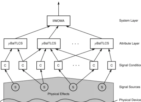
The MACRO approach is applied for the fusion of sev-eral sensor signal inputs. MACRO’s structure is depicted in Fig. 2.
The basic multilayer structure of this approach is in-spired by the decision-making process of groups of humans: individual humans (sensors) discuss their opinions (mea-surements) in groups (attribute layer). This group decision-making process includes conflicts. The information gener-ated in the various groups is then combined on an organ-isational level (system layer) to make a global decision. For more information on the human group decision-making background of MACRO, the reader is referred to Mönks and Lohweg (2013). It was shown that the application of this ap-proach for hazardous material store monitoring is beneficial compared to state-of-the-art installations (Ehlenbröker et al., 2014).
Figure 2.Multilayer attribute-based conflict-reducing observation system MACRO (Mönks and Lohweg, 2014).
the system as well as from its environment (like tempera-ture) are acquired by sensors (signal sources). Features are extracted from the signals in the followingsignal condition-ing step, which may also include signal preprocessing pro-cedures. Multiple features may be extracted from one signal, as shown in Fig. 2, e.g. to determine the mean and variance from one signal. Without loss of generality, the following as-sumes one feature per signal.
In the signal conditioning step, the sensor measurements, which may include all sorts of (physically) different types of measurements (e.g. temperature, air pressure), are trans-formed into a unitless space. A fuzzy set theory (Zadeh, 1965) approach has been chosen for modelling the acquired data in a common unitless space between 0 and 1. It is capa-ble of model uncertainty in the data, which is coming from, e.g., sensor noise, and allow variations in the system’s be-haviour due to environmental changes (e.g. in temperature, humidity), which do not affect the fulfilment of the sys-tem’s task. The Modified-Fuzzy-Pattern-Classifier (MFPC) (Lohweg et al., 2004) models the information by a uni-modal potential function applied as fuzzy membership func-tion µ:R→ [0,1]. This information model has proven its
performance scientifically as well as in real-world applica-tions (e.g. Lohweg et al., 2004; Niederhöfer and Lohweg, 2008; Mönks et al., 2010).
It employs an automatic learning procedure to determine the membership function based on measurement data:
Definition 2. Modified-Fuzzy-Pattern-Classifier learning (Lohweg et al., 2004; Mönks et al., 2010): the measure-ments of sensorSi at discrete time instance k∈N are
denoted as xi[k]. The vector xi=(xi[k]), 1≤k≤N
consists of the N individual measurements. Then the
measurements are represented by the
Modified-Fuzzy-Pattern-Classifier membership function as
µ(x,pi)=2−d(x,pi) (1)
withd(x,pi)=
|x−x
i| Ci
Di
.
The parameterspi=(xi, Ci, Di) are determined based
on the measurement dataxi by
xi=
1
N N
X
k=1
xi[k], Ci=
1
2·(max(xi)−min(xi)). (2)
The integer-valued parameterDi is chosen empirically,
typically as a power of 2 to keep computation of Eq. (1) hardware efficient.
Hence, the parameter vector p defines the membership
function’s properties: x is its mean value, C denotes the
width, andD determines the steepness of the membership
function. Sincep is automatically determined on the basis
of measurement data, the current condition is encoded in the parameters. In order to actually represent the normal condi-tion of the monitored system by p, the measurement data
must be acquired within a period of time, in which the sys-tem is operated in normal condition, which must be verified manually by a human expert, e.g. an experienced machine operator. Then the membership function is denoted asNµ. Please note: the fusion approach poses one demand on the applied sensors: the signals should be compatible to those during normal condition if the system does not change its be-haviour, whereas they need to change if the system changes its behaviour. Whether the sensors output signals represent the ground truth is irrelevant in this scope; hence, calibration is not necessary. Instead, the reaction on changes is impor-tant.
The fuzzy membership function is applied to compute the grade of membership Nµ
i(x)=Nµi(x,pi), to which a
sen-sor’s measurementx represents the normal condition. Note
that one membership function is utilised per sensorSi. An
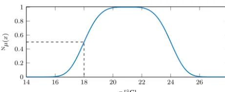
exemplary membership function for a temperature sensor is shown in Fig. 3.
14 16 18 20 22 24 26 28 0
0.2 0.4 0.6 0.8 1
x[◦C]
Nµ
(
x
)
Figure 3.Exemplary membership function for the normal condi-tion of a temperature sensor withx=21◦C,C=3◦C, andD=4. A measurement ofx=18◦C results in a membership of µ(x)= 0.5, as marked by the dashed lines.
solving (µBalTLCS) fusion approach (Lohweg and Mönks,
2010a; Mönks et al., 2012; Mönks and Lohweg, 2013). It cre-ates one output Nµ
a: [0,1]n→ [0,1] per attribute a from
its inputs. It additionally assigns each attribute an impor-tance measureIa∈ [0,1]. The importance measure is based
on the conflict between the sensors’ individual opinionsNµ
i.
Hence, the higher the conflict between an attribute’s inputs, the lower this attribute’s importance. The importance are em-ployed in the subsequent fusion of the attributes’ opinions Nµa, which are aggregated on a system level using the im-plicative importance-weighted ordered weighted averaging (IIWOWA) operator (Larsen, 1999) to reason about the en-tire system under supervision.
This operator is based on the importance-weighted ordered weighted averaging (IWOWA):
Definition 3. Importance-weighted ordered weighted aver-aging (Larsen, 1999): letµ=(µ1, µ2, . . ., µn) be a
vec-tor of fuzzy memberships, andI=(I1, I2, . . ., In) a
vec-tor of corresponding importance weights. The vecvec-tor of weights w=(w1, w2, . . ., wn) determines whether the
operator behaves more like the maximum or more like the minimum aggregation (more optimistic or more pes-simistic), with
n
X
j=1
wj=1 andρ(w)=1−
1
n−1 n
X
j=1
(n−j)·wj,
whereρ(w)∈ [0,1]determines the aggregation’s
and-ness degree. This is a measure indicating to which de-gree the operator behaves like the minimum operation. An andness of ρ(w)=0 represents a pure maximum, ρ(w)=1 a pure minimum operation. The operator is
able to model any degree of andness betweenρ=1 and ρ=0 (Yager, 1988). Then the class of IWOWA
opera-tors is defined as
hIWOWA(I,w,µ)= n
X
j=1
wj·b(j), (3)
with j∈Nn= {1,2, . . ., n}, and bj=ρ(w)+Ij· µj−ρ(w)
, where (·) denotes a permutation onbwith b(1)≥b(2)≥. . .≥b(n), i.e. the importance-weighted
memberships sorted in decreasing order.
Larsen (1999) showed in Larsen (1999) that the class of IWOWA operators is order equivalent to the weighted arith-metic mean (WAM) operator. Order equivalence is sufficient when the operator is applied to provide preference order-ing (Larsen, 2002). However, in situations where the aggre-gated value is used for other purposes, such as information fusion, full value equivalence to WAM is necessary. This property is obtained by normalising Eq. (3) in the interval ofhIWOWA(I,w,0) andhIWOWA(I,w,1). This leads to the following class of operators:
Definition 4. Implicative importance-weighted ordered weighted averaging (Larsen, 2002): let 0=(0, . . .,0)
be a vector of zeros and1=(1, . . .,1) a vector of ones,
each of lengthn. Then the class of IIWOWA operators
is defined with Eq. (3) as
hIIWOWA(I,w,µ)
=hIWOWA(I,w,µ)−hIWOWA(I,w,0)
hIWOWA(I,w,1)−hIWOWA(I,w,0). (4)
In the scope of MACRO, the result of
hIIWOWA(I,w,Nµ) is denoted system health Nh, with
Nµ=(Nµ1,Nµ2, . . .,NµA) being the attribute’s member-ships obtained byµBalTLCS fusion, andI=(I1, I2, . . ., IA)
the corresponding importances.
Detailed information regarding MACRO andµBalTLCSis found in Mönks et al. (2012); Mönks and Lohweg (2013), while optimisations concerning an efficient implementation are found in Mönks and Lohweg (2014). This contribu-tion concentrates on MACRO’s fusion on the attribute layer. Here, the sensor signals are fused initially and checked for consistency.
2.2 Monitoring of sensor reliability
Sensors are utilised in real-world applications to acquire sig-nals, which represent the current situation in the application. The IEEE standard 610-1990 defines “reliability” as follows:
Definition 5. Reliability (IEEE Computer Society, 1990, p. 170): “[t]he ability of a system or component to per-form its required functions under stated conditions for a specified period of time.”
Definition 6. Sensor reliability measure (Glock et al., 2011): the sensor reliability measure of sensorSi ∈S,i∈Nn
is defined as
ri=min
ris, rid, (5)
whereris denotes a sensor’s static and rid its dynamic
reliability.
Reliability is split in a static and a dynamic part. Static re-liabilityrisexpresses the probability that the sensor operates
correctly in general. Each sensor in a real-world application is exposed to external, inevitable effects like ageing, which affects its output signal such that it deviates from the actual situation of the application. In consequence, the sensor’s re-liability is affected over time. This is represented by the dy-namic partrid.
In order to compute the dynamic reliability, Glock et al. (2011) make use of the concepts of majority observation andconsistency. In Glock et al. (2011), information fusion for machine condition monitoring is considered. It employs multiple sensors acquiring their signals from the same ap-plication. The sensor outputs are approximations of the true value and hence prone to uncertainty, which is determined by each sensor’s characteristics. Therefore, each sensor’s mea-surement is considered by
Definition 7. Sensor observation (Glock et al., 2011): let
xi be the output of sensor Si. Then this measurement
is represented by the possibility distribution πi:R→ [0,1], which is denoted as sensor observation and
mod-els the sensor output’s characteristics for the given mea-surementxi.
Based on this, the degree of consistency between individ-ual observations is determined by
Definition 8. Consistency index (Glock et al., 2011): let
T ⊆Sbe a subset of sensorsSi∈S with their
respec-tive observationπi. Then the consistency index of their
observations is determined as
h(T)=sup x∈R
min
i|Si∈T (πi(x))
, (6)
withh(T)∈ [0,1]for allT.
A geometric interpretation of the consistency index is the height of the overlapping parts of all considered possibil-ity distribution functions, i.e. observations. In case the ob-servations of the employed sensors Si∈T are on
differ-ent measuremdiffer-ent scales, these need to be transformed to a common scale by fuzzification, hence a mapping µi:xi→ [0,1]. Such situations occur due to unequal dimensions
(two-dimensional image vs. one-(two-dimensional force) or physical
units (colour temperature in K vs. force in N). Thus, with-out fuzzification, the consistency index is not computable, whereas this measure is necessary to determine the majority observation. It is defined as
Definition 9. Majority observation (Glock et al., 2011): let 2Sbe the set of all subsets ofS. Then the set of sensors
Sm, determined by
Sm=
(
T
sup
T∈2S
(h(T)>0)
)
, (7)
forms the majority observation, if and only if|Sm|>1.
Considered geometrically, the observations of each mem-ber ofSmoverlaps with at least one other member ofSm. All
of their observations are considered fully consistent and span the range of the majority observation.
Although the remaining sensors {SrSm} do not
con-tribute to the majority observation, their observations are considered consistent to a certain degree. In order to quan-tify the consistency, Glock et al. (2011) proposed to relate the centres of gravity of each observationπi to the range of
the majority observation:
Definition 10. Majority consistency measure (Glock et al., 2011): letπi be the observation of sensorSi∈S. It is defuzzified by the centre of gravity method (Klir and Yuan, 1995, p. 336):
c(πi)= ∞
R
−∞
πi(x)·xdx
∞
R
−∞
πi(x) dx .
The range of the majority observation
cminm , cmmax is determined over the respective observations’ centres of gravity by
cminm = min i|Si∈Sm
(c(πi)), cmmax= max i|Si∈Sm
(c(πi)).
Then the majority consistency measure is defined as
Com(πi)=
cmmin−c(πi), c(πi)< cmmin, c(πi)−cmmax, c(πi)> cmmax,
1, otherwise.
(8)
If any of the observations overlap, no majority observa-tion is determined (|Sm| =1). In this case an average
Definition 11. Weighted arithmetic mean: let a=(ai) with ai∈R and i∈Nn be a vector of input values, and q=(qi) withqi∈Ra vector of corresponding weights.
Then the weighted arithmetic mean is determined by
λWAM(q,a)= n
P
i=1 qi·ai
n
P
i=1 qi
. (9)
Then the average consistency measure is defined as
Definition 12. Average consistency measure (Glock et al., 2011): letπi be the observation of sensorSi. For the
re-maining sensorsSjwithj 6=i, the vectorπ∗=(πj|j 6= i) contains the respective observations,r∗=(rj|j6=i)
contains the respective reliability measures after Eq. (5), andv∗=(vi,j|j6=i) contains the vicinity measures of
observationπi toπj, which is defined as
vi,j=1−c(πi)−c(πj) .
Then the average consistency measure is determined by
Coa(πi)= (10)
max
1− maxn
j=1|j6=i(rj), λWAM r ∗,v∗
,
if and only if no majority observation is determined; hence|Sm| =1.
This measure determines the average of the vicinities be-tweenπiandπj, weighed by the respective reliabilitiesrjin
the case of high reliabilities (rj →1 for allj). If the other
sensors are unreliable (rj→0 for all j), the observation
of sensor Si is considered consistent to the truth such that
Coa(πi)→1.
To summarise, the consistency measure for arbitrary ob-servations is defined by
Definition 13. Consistency measure (Glock et al., 2011): let
Sm denote the set of sensors, which form the major-ity observation after Definition 9. Then the consistency measure is determined by
Co(πi)=
Coa(πi), |Sm| =1,
Com(πi), otherwise. (11)
After introducing the concepts of majority observation and consistency, the dynamic sensor reliability is defined as
0 25 50 75 100
0 0.2 0.4 0.6 0.8 1
k
r
d[ki
]
ω= 0.01
ω= 0.1
ω= 0.5
Figure 4.Development of the dynamic reliabilityrid[k]of an ex-emplary sensorSiwithω= {0.01,0.1,0.5}. At the beginning of the
pictured period the measured value of the sensor drastically changes and is in conflict with other sensors.
Definition 14. Dynamic sensor reliability (Glock et al., 2011): let Co(πi) be the consistency measure of the
ob-servation of sensorSi ∈S. Then the dynamic sensor
re-liability at discrete time instancek∈Nis determined as
rid[k] =ω·Co(πi)+(1−ω)·rid[k−1], (12)
withrid[k] =1 for allk <0, andω∈ [0,1].
Glock et al. (2011) defined the dynamic reliability mea-sure in the form of an exponential moving averaging infi-nite impulse response filter (Meyer-Baese, 2007) to account for noise in the sensor observations and include information about the inertia of the monitored application by the smooth-ing factorω: in order to react fast to changes in application
with high inertia, the smoothing factor is set toω→1. In
low-inertia applications, signal changes occur faster and thus demandω→0 in order to mitigate the influence of
possi-ble outliers in the adjustment of the sensor’s reliability. An overview of the influence of ω on an exemplary dynamic
sensor reliability is shown in Fig. 4. The smoothing effect of small values forωis clearly visible.
2.3 Sensor defect detection
Sensor defects lead to sensor outputs, which do not represent the ground truth of the monitored system. In consequence, signals acquired by defective sensors result in information, which is in conflict with the information from intact sensors. These deliver signals, which represent the ground truth. Al-though the effects of conflicts in the input information is re-duced by theµBalTLCSfusion algorithm applied in MACRO, additional detection of sensor defects can be utilised to iden-tify and replace defective sensors. Then, conflicts between the acquired information vanish, which consequently leads to increased importance of the previously affected attributes. In order to facilitate sensor defect detection, the approach of Glock et al. (2011) for monitoring sensor reliabilities is utilised (cf. Sect. 2.2). The reliability of sensorSi is
time-dependent, part rid[k]. It is assumed that the sensor is
reliable at the beginning of the monitoring and hence set to
ris=1. If additional information is available regarding static
reliability, this value may be adjusted. Since the dynamic part of the sensor reliability is time dependent, the whole measure is time dependent. Based on this, a sensor defect is detected, when its reliability measureri[k]falls below a certain
thresh-old:
Definition 15. Sensor defect decision rule: let ri[k]be the
reliability of sensorSi∈S at discrete time instancek.
The average reliability of all sensors is computed as
r[k] =1 n
n
X
i=1 ri[k].
Then a sensor defect is determined by evaluating the sensor defect decision rule:
ri[k]< η·r[k] ⇒sensorSiis defective, (13)
whereη∈ [0,1]controls the decision threshold.
The decision threshold is designed variable with respect to
r[k]to mitigate wrong decisions in real-world applications.
If the monitored application changes its behaviour over time, this is not necessarily detected by all sensors at the same time. Hence, the observations of a subset of sensors become inconsistent and the respective reliabilities are decreased al-though no sensor defects occurred. After some time, all sen-sors that are contributing to one attribute, detect the change of the system leading to an equilibrated situation: sensor ob-servations are consistent such that the previously decreased reliabilities increase again. If the decision threshold was con-stant in this case, a number of sensors would be declared as defective for some time and later as intact again.
Besides introducing a sensor defect decision rule, this con-tribution adapts the approach of Glock et al. (2011) to deter-mine the individual reliabilities within groups of sensors.
Definition 16. Groupwise sensor reliability measure: the in-dividual sensor reliability measure is determined on the basis of consistency evaluations among groups of sen-sors. These sensor groups are defined such that their sensors acquire signals influenced by the same property or constituent part of the monitored application. Each sensor group is a subset of all sensors denoted asSg⊆S
withg∈N, where an individual sensorSi is a member
of one or more groups of sensorsSg. Consequently, the
groupwise sensor reliability measure is determined as
ri[k] =
1
G G
X
g=1
ri,g[k], (14)
whereri,g is the sensor reliability measure of sensorSi
in groupgdetermined after Eq. (5) withS→Sg, and Gdenotes the number of sensor groups Sg, to which
sensorSi is assigned.
This groupwise procedure is motivated due to several as-pects:
– The sensors’ signals inheritsemanticorspatial proximi-ties, as they are influenced by the same property (seman-tic proximity) or constituent part (spatial proximity). If the signals are influenced by a property, which is limited to one constituent part, semantic and spatial proximity occur at the same time.
– Due to said proximities, no coincidental correlations tween independent signals occur. Causal relations be-tween the signals inside one group are trustworthy.
– Applied within the context of MACRO, the required sensor groups are already defined as attributes. Hence, no further effort needs to be invested.
Although the application within the context of MACRO is beneficial, the approach is not restricted to it. It is applicable wherever grouping of sensors is possible. If no grouping is possible and all sensors need to be evaluated at once, the ap-proach is also applicable: in this case only one group exists.
The approach of Glock et al. (2011) for monitoring sen-sor reliabilities is based on possibility distributionsπi, which
model the sensor characteristics with respect to measurement uncertainties given outputxi. It is assumed to be available
for each sensor in their approach. To the best knowledge of the authors, such information does not exist for any (non-)commercially available sensor. Thus, it must be determined manually for each sensor in order to make the approach us-able in real-world applications, for which the following prac-ticable procedure is proposed:
Definition 17. Determination of sensor observation: the characteristics of sensor Si in terms of measurement
uncertainty with respect to its current outputxi is
ex-pressed by the probability density function (pdf)pxi. If no other pdf is predetermined, it is assumed to be a uniform pdf on the interval[a, b]:
pxi(x)=
1
b−a, a≤x≤b,
0, otherwise.
The interval[a, b]limits the maximum measurement
er-ror of sensorSi in case ofxi. It is either available from
the sensor’s data sheet, determined experimentally, or is approximated sensibly by an expert.
triangular probability–possibility transform (Lasserre et al., 2000; Mauris et al., 2000), which also allows for the transfer of Gaussian, triangular and Laplacian pdfs. This procedure is carried out separately for each mea-surement xi. The foundations of the truncated triangular
probability–possibility transform are not included in this contribution since it is only applied and Lasserre et al. (2000) and Mauris et al. (2000) provided excellent introductions to it.
In order to determine the consistency measure for arbitrary sensors, their measurement scales are fuzzified before trans-formingpxi toπi.
Definition 18. Fuzzification of sensor measurement scales: with respect to MACRO, the fuzzification of the sensors’ measurement scales is delivered through Modified-Fuzzy-Pattern-Classifier learning (cf. Defini-tion 2) by Nµi :
R→ [0,1] for sensor Si. Then the
sensor characteristics functionpxi:R→ [0,1]is
trans-ferred toNpx
i: [0,1] → [0,1]with
Np
xi Nµi(x) =
pxi(x). (15)
Consequently, the sensor observationπi :R→ [0,1]is
transferred toNπi: [0,1] → [0,1]with
Nπ
i Nµi(x)=πi(x). (16)
The fuzzification through MFPC learning is already avail-able as it is applied in MACRO for fusion on the attribute layer. Hence, the integration of arbitrary sensors is achieved in MACRO without any extra effort. In order to assist read-ability, Nπi=Nπi Nµi(x)
is applied in the following. An exemplary sensor observation determined on fuzzified mea-surement scales is visualised in Fig. 5.
In addition, fuzzification has implications on the determi-nation of the consistency index (cf. Eq. 6). Without fuzzi-fication the whole range of real numbers is necessary to be evaluated (x∈R), whereas due to fuzzification, the unit
in-terval is evaluated (Nµ
i(x)∈ [0,1]).
From the following example, the necessity of an adapta-tion of the majority consistency measure as defined in Eq. (8) and Glock et al. (2011) is revealed.
Example 1. Properties of the majority consistency measure: regardless of the fuzzification of the measurement scale, let the centres of gravity of the following two observa-tions be
c(π1)=cmaxm +ε, c(π2)=cmmin−ε,
with 0< ε1. Thus, both observations are close to
the borders of the majority observation. Then the cor-responding majority consistency measures are
Com(π1)=ε,Com(π2)=ε.
26 26.2 26.4 26.6 26.8
0 0.5
1 1.5 2
x[N]
px1
(
x
)
0.9 1 1.1
0 2 4 6
x[A]
px
2
(
x
)
(a) (b)
24 26.4 30 33 0
0.43 1
x[N]
Nµ
1
(
x
)
0 1 2 2.5
0 0.5
1
x[A]
Nµ
2
(
x
)
(c) (d)
0 0.1 0.2 0.3 0.4 0.5 0.6 0.7 0.8 0.9 1
0 0.2 0.4 0.6
0.81
Nµ i(x) Nπ
i
Nµ
i
(
x
)
(e)
Figure 5.Exemplary determination of the sensor observationsNπ1
andNπ2on fuzzified measurement scales. The plots depict the
re-spective functions of sensorS1measuring a force in N in blue, and
those of sensorS2measuring an electric current in A in red. Note
the incomparable measurement ranges and physical units, which are transformed step-by-step from(a)to(e)into a common space (a,b:
sensor characteristics at measurement valuexi(given by the dashed
stem) represented by uniform probability density functions;c, d:
fuzzy membership functionsNµi modelling the normal condition
as acquired by the respective sensor along with the fuzzified mea-surement value (given by the dashed line);esensor observations as
determined by the truncated triangular probability–possibility trans-form on the common fuzzified measurement scale along with the respective fuzzified measurement (given by the dashed stems)). The majority observation is visible in(e)in the overlapping region of
the two functions.
Now let
c(π10)=cmaxm +ε0, c(π20)=cminm −ε0,
withε0> εbeing two observations further away from
the majority observations’ borders compared toπ1and π2. Then
Com(π10)=ε0>Com(π1),Com(π20)=ε0>Com(π2).
The preceding example shows that the majority consis-tency measure increases with increasing distance of an ob-servation to the majority obob-servation. Contrarily, the major-ity consistency measure was defined in Glock et al. (2011) to be decreasing with increasing distance to the majority obser-vation.
Glock et al. (2011) deduced Com(πi)∈ [0,1) for all i.
c(πi)=cmaxm +1, where1∈R, are valid and possible. This
leads to Com(πi)>1 for1 >1.
Therefore, the majority consistency measure is proposed to be adapted:
Definition 19. Adapted majority consistency measure: let Nπi be the observation of sensorSi∈S on a fuzzified scale according to Eq. (16). Then the adapted majority consistency measure is defined as
Com Nπi= (17)
1− cminm −c Nπi
, c Nπi
< cminm ,
1− c Nπi
−cmaxm , c Nπi
> cmaxm ,
1, otherwise,
with Com Nπi∈ [0,1]for alli. It is a measure, which
decreases with increasing distance of an observation to the majority observation.
All necessary parts for sensor defect detection are now available. To summarise, the sensor defect detection ap-proach proposed in this section
– is based on the sensor reliability monitoring approach presented in Glock et al. (2011);
– demands fuzzification of the measurement scales in all cases, which is delivered at no additional cost in the con-text of MACRO;
– determines observation consistency within groups of sensors, which are delivered at no additional cost in the context of MACRO;
– adapts the majority consistency measure defined in Glock et al. (2011).
3 Experiments and results
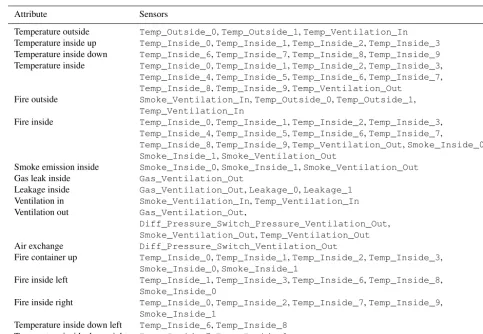
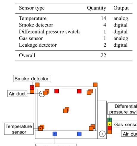
In this section, the defect detection results under normal op-erating conditions are presented first. Afterwards it is shown that the defect detection also works when the monitored sys-tem is not in a normal operating state. The capabilities of the sensor fault detection approach for different fault types are finally shown. The real-world use case is a hazardous mate-rial store from the research project itsowl-IGel (itsowl-IGel, 2015). Different types of sensors are applied, which are listed in Table 1.
For the detection of leakages, electro-optical switches are used; they are activated when the measuring tip is surrounded by liquid and are placed at the bottom of the hazardous ma-terial store. The sensors are combined into 17 attributes and are positioned on the inside, the air ducts (ventilation), and the outside of the hazardous material store. A schematic view of the store and the used sensors is given in Fig. 6.
The attributes are listed in Table A1. Some attributes are defined manually based on their location (e.g. ventilation in),
Table 1.List of all sensors applied to the hazardous material store.
Sensor type Quantity Output Temperature 14 analog Smoke detector 4 digital Differential pressure switch 1 digital
Gas sensor 1 analog
Leakage detector 2 digital
Overall 22
Figure 6.A schematic view of the hazardous material store with the sensors included. The different sensors are shown in different colours (temperature sensor: orange; smoke detector: red; leakage detector: blue; gas sensor: yellow; differential power switch: green). Additionally the air ducts are marked.
with some attributes also being defined based on their se-mantics (e.g. leakage). Others are a combination of the two aforementioned approaches (e.g. fire inside).
For the experiments, ω is set to 0.01 to avoid sudden
changes in the computation of dynamic reliabilitiesrid due
to outliers (cf. Fig. 4 forω=0.5). The data and detailed
con-figuration used for these experiments are available via Ehlen-bröker et al. (2016a).
3.1 Defect detection under normal operating conditions Sensor data were gathered in a hazardous material store demonstrator, which has been built for the itsowl-IGel project, under the following conditions: the hazardous ma-terial store was in a normal operating state with tem-peratures around 25◦C, whereas one temperature sensor
(Temp_Inside_8) was delivering incorrect values (140 to
150◦C).
As can be seen in Fig. 7, the sensor defect is clearly tectable, as the sensor’s reliability falls below the defect de-cision threshold.
ex-0 10 20 30 40 50 60 0
0.2 0.4 0.6 0.8 1
t[min] (∝k)
r
[
k
]
Temp_Inside_8 Defect decision threshold
Figure 7.The defect decision threshold (η=0.75) and the
reliabil-ityr[k]of the defective sensorTemp_Inside_8with a random error (ω=0.01).
periment, the measurements ofTemp_Inside_8are again more consistent with the values of the other sensors and con-sequently the reliability increases.
3.2 Defect detection during non-normal operating conditions
To demonstrate that the detection of a sensor defect is also possible, if the hazardous material store is in a critical state, a smoke detector is falsely activated during an actual leak-age in the store. Leakleak-ages occur, e.g., after a container with chemicals was damaged during the handling of the contain-ers. As the stored chemicals are often toxic or flammable, it is important to reliably detect leakages, in spite of possible sensor defects.
The leakage in this scenario is an ongoing process: a dam-aged container releases its fluid content, which begins to gather itself at the bottom of the hazardous material store. At the same time parts of the leaking fluid evaporate and are detected by the gas sensor. The detection of the leaked fluids at the bottom of the store takes a longer time, as the leakage detectors only detect larger quantities of fluid.
The defective smoke detector was falsely activated after 3:00 min. This results in a steady decrease of this sensor’s reliability, as displayed in Fig. 8. The defect of this sensor was detected at around 5:30 min, when the sensor’s reliability crossed the defect decision thresholdη.
AlthoughSmoke_Inside_0delivered incorrect values, the critical system state caused by the leakage is reliably rep-resented in the decreasing system healthNh[k](cf. Eq. 4), as can be seen in Fig. 9.
The system health develops stepwise, with the first drop at about 3:00 min caused by the defect of the smoke detec-tor. The following two drops are caused by the gas detector, which detects a gas leakage (at about 8:00 min), and the two leakage detectors activating at around 13:00 min. The visible jitter of the system health is caused by fluctuating measure-ments of the gas sensor.
0 2 4 6 8 10 12 14 16
0 0.2 0.4 0.6 0.8 1
t[min] (∝k)
r
[
k
]
Smoke_Inside_0 Defect decision threshold
Figure 8.The defect decision threshold (η=0.75) and the
reliabil-ityr[k]of the defective sensorSmoke_Inside_0(ω=0.01).
0 2 4 6 8 10 12 14 16
0 0.2 0.4 0.6 0.8 1
t[min] (∝k) Nh
[
k
]
System health Alarm threshold Warning threshold
Figure 9.The system healthNh[k]of the monitored system during a leakage over time. It is the aggregated result of the fusion process on system level (cf. Eq. 4) and represents the state of the store. The depicted warning and alarm thresholds were manually set. They are used for the generation of alarms for operators.
3.3 Defect detection of different fault types
In the following an overview about the detection of four sensor fault types with different strengths is given. For this evaluation, a multi-hour data recording of sensor
Temp_Inside_2from the hazardous material store in
nor-mal operation has been superposed with the following typical defects (cf. Helwig et al., 2015):
Peaks: Sensor reading outliers are simulated by adding 100◦C at random time instances with rates between 1
and 10 peaks per minute.
Offset: Sensor values are evaluated at constant offsets be-tween 1 and 5◦C.
Drift: Drifting sensor data are evaluated for constant rates between 1 and 5 ‰ h−1.
Noise: Additive zero-mean Gaussian noise is evaluated for signal-to-noise ratios (SNR) of 10 and 0 dB.
Defect decision thresholdηandωare set identical to the
previously used values (η=0.75,ω=0.01). The data and
0 0.5 1 1.5 2 2.5 3 3.5 4 4.5 5 0
0.2 0.4 0.6 0.8 1
t[min] (∝k)
r
[
k
] No peaks 1Peak min 2Peaks min 5Peaks min 10Peaks min
Defect -1
-1
-1 -1
Figure 10.Reliability and detected defects for peak sensor faults. Peaks are randomly inserted to the measurement with frequencies from 1 to 10 peaks per minute by adding 100◦C to the original
sensor readings. The detected defect is marked by a red dot.
0 20 40 60 80 100 120
0 0.2 0.4 0.6 0.8 1
t[s] (∝k)
r
[
k
]
No offset 1◦C offset
2◦C offset
5◦C offset Defect
Figure 11.Reliability and detected defects for offset sensor faults. Results are shown for constant offsets between 1 and 5◦C. Detected
defects are marked by a red dot.
The evaluation results in terms of sensor reliabilities are depicted in Figs. 10–13. For reference, the sensor reliability without a defect is included in each figure. It is visible that these fault-free cases are correctly detected to include no de-fect.
Figure 10 shows the performance of the proposed algo-rithm for peak errors. No defects are detected up to a peak frequency of 5 peaks per minute, whereas a defect is detected at 1 min running time at a level of 10 peaks per minute.
Results on offset faults are shown in Fig. 11. An offset of 1◦C remains undetected, whereas it takes around 75 and 35 s
to detect 2 and 5◦C offsets, respectively.
The defect detection behaviour for peaks and offset is due to the exponential averaging of the sensor reliability. It allows sensor behaviour deviations to a certain extent, which does not imply an actual defect. Its sensitivity is adjusted byω.
For drift errors, the detection is dependent on the length of the observed period: a drift fault of 5 ‰ h−1, as depicted in
Fig. 12, is detected after 10 h. The detection of a drift error of 2 ‰ h−1takes 16 h. The drift fault of 1 ‰ h−1is not detected
during the monitored time period.
0 2 4 6 8 10 12 14 16 18 20
0
0.2
0.4
0.6
0.8
1
t[h] (∝k)
r
[
k
]
No drift
1‰ h
2‰ h
5‰ h
Defect -1 -1 -1
Figure 12.Reliability and detected defects for drift sensor faults. Results are shown for drift rates between 1 and 5 ‰ h−1. Detected
defects are marked by a red dot.
0 0.5 1 1.5 2 2.5 3 3.5 4 4.5 5
0.96 0.98 1
t[h] (∝k)
r
[
k
]
No noise
SNR10dB
SNR0dB
Figure 13.Reliability and detected defects for noise sensor faults. The evaluated signals contain additive zero-mean Gaussian noise with signal-to-noise ratios (SNR) of 10 and 0 dB. No defect is de-tected.
Figure 13 depicts the results for noise faults. As is seen in the figure, no noise faults are detected. Compared to other sensor faults, the reliability decreases tor=0.985 on
aver-age for the signal containing maximal noise (SNR 0 dB). The detection behaviour for the latter two defect types at-tributed to the fact that the MACRO information fusion ap-proach, on which this sensor defect approach is based. It is geared to be tolerant towards signal variations and noise in order to show stable behaviour to real-world system varia-tions and prevent wring decisions. However, its sensitivity is adjusted by manual adjustments of the membership func-tions’ widthsCi.
4 Conclusion and outlook
This paper presents a method to generate a consistency-based reliability assessment for sensors, which is utilised to de-tect sensor defects. The approach is embedded into the in-formation fusion system MACRO, which is well-suited for the implementation of the proposed sensor defect detection approach. As MACRO combines sensors in attributes, sen-sor groups with semantic and/or spatial proximity, which are primed to be used in the proposed consistency-based defect detection approach, are already employed. However, the ap-proach is applicable also in the context of other information fusion applications. It was shown that the approach is capable of detecting sensor defects. The tests were carried out in the context of two real-world examples, in which a hazardous material store was monitored during normal operation and during a leakage. It was possible to detect the sensor defects in both scenarios. Additional tests for typical sensor defect types evaluate the defect detection approach with respect to peak, offset, drift, and noise. It is shown that defect detection is in general possible.
Sensor defects directly influence the conflict between sensor inputs. Hence, the conflict (which is the attribute’s negated importance in the context of MACRO, delivered at
no additional cost) seems to be an appropriate indicator for a possible sensor defect. It is to be investigated, whether this is exploitable to determine and assess sensor reliabilities only in cases, where the conflict exceeds a certain level. The pre-sumably saved computational resources and effects on the defect detection’s accuracy are to be evaluated. Further, a de-tailed look into more complex scenarios is of interest: defects of multiple sensors have not been considered, yet. If nec-essary, the proposed defect decision rule and the groupwise sensor reliability measure will be adapted. An investigation of false-positive and false-negative defect detection rates and the identification of optimisation possibilities of said rates needs also to be carried out. As the presented approach is in-sensitive to sensor faults of small values, an investigation of changes to detect additional sensor faults is also of impor-tance.
5 Data availability
Appendix A: Attributes
The list of all attributes and their associated sensors is presented in Table A1.
Table A1.List of all attributes and their associated sensors. Attributes are named according to their position (e.g. outside, inside up, ventila-tion in). Addiventila-tionally, most attributes also include a monitored physical property (e.g. temperature) or semantics (e.g. fire).
Attribute Sensors
Temperature outside Temp_Outside_0,Temp_Outside_1,Temp_Ventilation_In
Temperature inside up Temp_Inside_0,Temp_Inside_1,Temp_Inside_2,Temp_Inside_3
Temperature inside down Temp_Inside_6,Temp_Inside_7,Temp_Inside_8,Temp_Inside_9
Temperature inside Temp_Inside_0,Temp_Inside_1,Temp_Inside_2,Temp_Inside_3,
Temp_Inside_4,Temp_Inside_5,Temp_Inside_6,Temp_Inside_7,
Temp_Inside_8,Temp_Inside_9,Temp_Ventilation_Out
Fire outside Smoke_Ventilation_In,Temp_Outside_0,Temp_Outside_1,
Temp_Ventilation_In
Fire inside Temp_Inside_0,Temp_Inside_1,Temp_Inside_2,Temp_Inside_3,
Temp_Inside_4,Temp_Inside_5,Temp_Inside_6,Temp_Inside_7,
Temp_Inside_8,Temp_Inside_9,Temp_Ventilation_Out,Smoke_Inside_0,
Smoke_Inside_1,Smoke_Ventilation_Out
Smoke emission inside Smoke_Inside_0,Smoke_Inside_1,Smoke_Ventilation_Out
Gas leak inside Gas_Ventilation_Out
Leakage inside Gas_Ventilation_Out,Leakage_0,Leakage_1
Ventilation in Smoke_Ventilation_In,Temp_Ventilation_In
Ventilation out Gas_Ventilation_Out,
Diff_Pressure_Switch_Pressure_Ventilation_Out,
Smoke_Ventilation_Out,Temp_Ventilation_Out
Air exchange Diff_Pressure_Switch_Ventilation_Out
Fire container up Temp_Inside_0,Temp_Inside_1,Temp_Inside_2,Temp_Inside_3,
Smoke_Inside_0,Smoke_Inside_1
Fire inside left Temp_Inside_1,Temp_Inside_3,Temp_Inside_6,Temp_Inside_8,
Smoke_Inside_0
Fire inside right Temp_Inside_0,Temp_Inside_2,Temp_Inside_7,Temp_Inside_9,
Smoke_Inside_1
Temperature inside down left Temp_Inside_6,Temp_Inside_8
Acknowledgements. This article is based on the SENSOR 2015 conference contribution by the same authors (Ehlenbröker et al., 2015). The authors would like to thank Denis Petker for the helpful remarks and valuable help during the preparation of this contribution. Additionally, we would like to thank Udo Roth and the Denios AG for the development and provisioning of the hazardous material store demonstrator, and their support during the real-world tests. This work was partly funded by the German Federal Ministry of Education and Research (BMBF) under grant agreement no. 02PQ2112, within the Leading-Edge Cluster “Intelligent Technical Systems OstWestfalenLippe” (it’s OWL).
Edited by: K.-D. Sommer
Reviewed by: three anonymous referees
References
Alpaydın, E.: Introduction to Machine Learning, Adaptive compu-tation and machine learning, MIT Press, Cambridge, MA, 2nd Edn., 2010.
Bay, S. D. and Schwabacher, M.: Mining distance-based outliers in near linear time with randomization and a simple pruning rule, in: The Ninth ACM SIGKDD International Conference, edited by: Senator, T., Domingos, P., Faloutsos, C., and Getoor, L., p. 29, doi:10.1145/956750.956758, 2003.
Bishop, C. M.: Pattern recognition and machine learning, Informa-tion science and statistics, Springer, New York, NY, 8th Edn., 2009.
Choi, S. W., Lee, C., Lee, J.-M., Park, J. H., and Lee, I.-B.: Fault detection and identification of nonlinear processes based on kernel PCA, Chemometr. Intell. Lab., 75, 55–67, doi:10.1016/j.chemolab.2004.05.001, 2005.
Dempster, A. P.: Upper and lower probabilities induced by a multivalued mapping, Ann. Math. Stat., 38, 325–339, doi:10.1214/aoms/1177698950, 1967.
Dubois, D. and Prade, H.: Fuzzy sets and probability: mis-understandings, bridges and gaps, 2nd IEEE Interna-tional Conference on Fuzzy Systems, 2, 1059–1068, doi:10.1109/FUZZY.1993.327367, 1993.
Duquet, S.: Smart Sensors: Enabling Detection and Ranging for the Internet of Things and Beyond, Elektronik Praxis, April 2015. Ehlenbröker, J.-F., Mönks, U., Wesemann, D., and Lohweg, V.:
Condition Monitoring for Hazardous Material Storage, 19th IEEE Int. Conf. on Emerging Technologies and Factory Automa-tion (ETFA 2014), Barcelona, Spain, 16–19 September 2014, 1– 4, doi:10.1109/ETFA.2014.7005264, 2014.
Ehlenbröker, J.-F., Mönks, U., and Lohweg, V.: Consistency Based Sensor Defect Detection, in: SENSOR 2015, AMA Ser-vice GmbH, Nürnberg, Germany, 19–21 May 2015, 878–883, doi:10.5162/sensor2015/P10.4, 2015.
Ehlenbröker, J.-F., Mönks, U., and Lohweg, V.: Sensor Defect Detection Datasets with Configuration, Zenodo, doi:10.5281/zenodo.48728, 2016a.
Ehlenbröker, J.-F., Mönks, U., and Lohweg, V.: Typical Sensor De-fects Dataset, Zenodo, doi:10.5281/zenodo.56358, 2016b. Elouedi, Z., Mellouli, K., and Smets, P.: Assessing Sensor
Re-liability for Multisensor Data Fusion Within the Transfer-able Belief Model, IEEE T. Syst. Man. Cy. B, 34, 782–787, doi:10.1109/TSMCB.2003.817056, 2004.
Glock, S., Voth, K., Schaede, J., and Lohweg, V.: A Framework for Possibilistic Multi-source Data Fusion with Monitoring of Sen-sor Reliability, in: World Conference on Soft Computing, San Francisco, USA, 23–26 May, 2011.
Hall, D. L. and Llinas, J. (Eds.): Handbook of Multisensor Data Fusion – The electrical engineering and applied signal process-ing series, CRC Press, Boca Raton FL, http://site.ebrary.com/lib/ alltitles/docDetail.action?docID=10142823, 2001a.
Hall, D. L. and Llinas, J.: Multisensor Data Fusion, in: Hand-book of Multisensor Data Fusion, edited by: Hall, D. L. and Llinas, J., pp. CRC Press, Boca Raton FL, 1-1–1-10, doi:10.1201/9781420038545.pt1, 2001b.
Helwig, N., Pignanelli, E., and Schütze, A.: Detecting and Compen-sating Sensor Faults in a Hydraulic Condition Monitoring Sys-tem, in: SENSOR 2015, AMA Service GmbH, Nürnberg, Ger-many, 1–21 May 2015, 641–646, doi:10.5162/sensor2015/D8.1, 2015.
Hu, Y., Chen, H., Xie, J., Yang, X., and Zhou, C.: Chiller sensor fault detection using a self-Adaptive Principal Com-ponent Analysis method, Energ. Buildings, 54, 252–258, doi:10.1016/j.enbuild.2012.07.014, 2012.
IEEE Computer Society: IEEE Standard Computer Dictio-nary: A Compilation of IEEE Standard Computer Glos-saries – IEEE Std 610-1990, IEEE, New York, NY, USA, doi:10.1109/IEEESTD.1991.106963, 1990.
itsowl-IGel: Intelligentes Frühwarnsystem für Gefahrstofflager (Intelligent early warning system for hazardous material storage areas): Research Project sponsored by the Fed-eral Ministry of Education and Research, available at: http://www.its-owl.de/projekte/innovationsprojekte/details/ intelligentes-fruehwarnsystem-fuer-gefahrstofflager/, 2015. Jaynes, E. T.: Probability Theory: The Logic of Science, Cambridge
Univ. Press, Cambridge, 727 pp., 2003.
Kerschen, G., Boe, P. D., Golinval, J.-C., and Worden, K.: Sensor validation using principal component analysis, VTT Symp., 14, 36 pp., doi:10.1088/0964-1726/14/1/004, 2005.
Khaleghi, B., Khamis, A., Karray, F. O., and Razavi, S. N.: Multi-sensor data fusion: A review of the state-of-the-art, Inform. Fu-sion, 14, 28–44, doi:10.1016/j.inffus.2011.08.001, 2011. Klir, G. J. and Yuan, B.: Fuzzy Sets and Fuzzy Logic: Theory and
Applications, Pentice Hall, New Jersey, 1995.
Krüger, M.: Gradual vs. binary conflicts in Bayesian networks ap-plied to sensor failure detection, 18th International Conference on Information Fusion, 2015, Washington, DC, 6–9 July 2015, 66–73, 2015.
Kusiak, A. and Song, Z.: Sensor Fault Detection in Power Plants, J. Energ. Eng.-ASCE, 135, 127–137, doi:10.1061/(ASCE)0733-9402(2009)135:4(127), 2009.
Larsen, H. L.: Importance weighted OWA aggregation of multicriteria queries, 18th International Conference of the North American Fuzzy Information Processing Society (NAFIPS 1999), New York, NY, 10–12 Jun 1999, 740–744, doi:10.1109/NAFIPS.1999.781792, 1999.
![Figure 4. Development of the dynamic reliabilityemplary sensorpictured period the measured value of the sensor drastically changes rdi [k] of an ex- Si with ω = {0.01,0.1,0.5}](https://thumb-us.123doks.com/thumbv2/123dok_us/965122.1595864/8.612.311.545.69.158/figure-development-dynamic-reliabilityemplary-sensorpictured-measured-drastically-changes.webp)

![Figure 7. The defect decision threshold (ityerror (η = 0.75) and the reliabil- r[k] of the defective sensor Temp_Inside_8 with a randomω = 0.01).](https://thumb-us.123doks.com/thumbv2/123dok_us/965122.1595864/12.612.311.546.245.340/figure-decision-threshold-ityerror-reliabil-defective-inside-randomw.webp)