Article
Two-Level Evolutionary Multi-Objective
Optimization of a District Heating System with
Distributed Cogeneration
Melchiorre Casisi1,*, Stefano Costanzo2, Piero Pinamonti1, Mauro Reini3
1 Polytechnic Dept. of Engineering and Architecture, University of Udine, Italy
2 ESTECO S.p.A., Area Science Park, Padriciano 99, Trieste, Italy
3 Dept. of Engineering and Architecture, University of Trieste, Italy
* Correspondence: [email protected]; Tel.: +39-338-9946-864
Abstract: The paper deals with the modelization and optimization of an integrated multi-component energy system. On-off operation and presence-absence of multi-components must be described by means of binary decision variables, besides equality and inequality constraints; furthermore, the synthesis and the operation of the energy system should be optimized at the same time. In this paper a hierarchical optimization strategy is used, adopting a genetic algorithm in the higher optimization level, to choose the main binary decision variables, whilst a MILP algorithm is used in the lower level, to choose the optimal operation of the system and to supply the merit function to the genetic algorithm. The method is then applied to a distributed generation system, which has to be designed for a set of users located in the center of a small town in the North-East of Italy. The results show the advantage of distributed cogeneration, when the optimal synthesis and operation of the whole system are adopted, and significant reduction in the computing time by using the proposed two-level optimization procedure.
Keywords: District Heating; multi-objective evolutionary optimization; distributed cogeneration; optimal operation.
1. Introduction
A more thorough integration among energy systems is expected to significantly contribute to reducing primary energy consumption, as well as global pollutant emissions and energy costs for final users. Integrated District Heating (DHN) networks and Combined Heat and Power (CHP) are of particular interest for the object of defining an efficient system for distributed energy generation and are widely discussed in Literature, i.e. in terms of role and opportunities in a country like Denmark [1] or United Kingdom [2], or considering a review of the different technology opportunities [3] and of the energy sources [4] also for Combined Heat, Cooling and Power systems (CHCP). The expected advantages of energy integration can, in fact, be obtained in real world applications only if the structure (synthesis) and the management of the whole system are carefully optimized. For instance, in [5] a computational framework is proposed to face the problem at city districts level, in [6] a Mixed Integer Linear Programming (MILP) model is used to determine the type, number and capacity of equipment in CHCP systems installed in a tertiary sector building, in [7] a modelling and optimization method is developed for planning and operating a CHP-DH system with a solar thermal plant and a thermal energy storage, in [8] a detailed optimization model is presented for planning the short-term operation of combined cooling, heat and power (CCHP) energy systems, for a single user in [9]an algorithm for the minimization of a suitable cost function is applied to optimize CHP commercial and domestic systems with variable heat demand.
Synthesis and operation optimization of integrated multi-component energy systems generally require a binary variable set to be introduced to describe the existence/absence and the on/off operation status of components and energy connections inside the model. Besides these, other
continuous variables have to be introduced for modelling the energy and material flows exchanged among components, as well as other possible design options [6, 10, 11].
In addition to this complex variable set, the variation of the thermal demands of the final users has also to be taken into account. Thus, a Mixed Integer Non Linear Programming (MINLP) problem has generally to be solved for obtaining the optimal synthesis and operation of the integrated system, with a high computational effort. A general introduction to MILP, MINLP and other possible approaches to the design and synthesis optimization of energy systems can be found in [12]. Recently, the MINLP approach has been used, for instance in [13, 14] to optimize the CCHP systems of different buildings with solar energy integration.
The computational effort can be reduced if the whole problem is faced by defining two (or more) levels, which can be solved dealing with a reduced number of independent variables [15], or if it is decomposed into many sub-problems, which have to be solved with an iterative procedure [16-18]. In both cases the solution could be more easily obtained if the problem were described with sufficient precision by means of a linear model (MILP), even if additional variables are introduced for considering strong non-linear relations among flows of both energy and mass [10, 11].
Unfortunately, when there is a high number of binary variables present in almost all sub-problems, the coupling variables, which allow each sub-problem to be solved consistently with the optimal solution of the whole system [19, 20], become too changeable to allow the convergence of the optimization process toward the actual optimum. This is highlighted, for instance, in [21], where the Mixed Integer Linearized Exergoeconomic (MILE) method is presented and the thermoeconomic costs are used as coupling variables.
In the present paper, such difficulties are overcome by using a novel approach, characterized by a two-level hierarchical optimization strategy which does not require an explicit system decomposition. In the proposed method a genetic algorithm is used in the higher optimization level, to choose the main binary decision variables, whilst a MILP algorithm is used in the lower level, to choose the optimal operation of the system and to supply the merit function to the genetic algorithm.
The proposed system model is intended for district-level implementation and is concerned with the optimal layout and operation of CHP units, deployed in different buildings, as well as with the optimal configuration of one, or more micro-district heating grids. A central CHP plant, besides a set of micro-CHP gas turbines distributed among the involved buildings, along with the installation of thermal collectors and photovoltaic (PV) panels have been considered to further improve the energy efficiency and sustainability of the whole system.
The main optimization was aimed at minimizing the total annual cost for owning, maintaining and operating of the whole system. Furthermore, the optimal solution, beside satisfying the electric energy and heating demands of each building throughout the year, should allow a minimum environmental impact. Therefore, a multi-objective optimization has been performed, by considering, as a second objective of the optimization, the avoided CO2 compared to the conventional energy
supply.
In summary, the method allows the identification of the optimal configuration of the micro-district heating grids, of the design of the CHP units in each building and the optimal operation of the whole energy system inside a unique optimization procedure, satisfying the energy demands of multiple users.
The focus of this paper does not lie so much in the numerical solution of the case study, but rather in the performance of the hierarchical optimization algorithm and on the option of easily performing a multi-objective optimization. The expectation is that the developed optimization strategy highlights a reduction in the computing time compared with the direct implementation of the whole problem in a single level MILP solver. Therefore, the presented method could be applied to distributed cogeneration systems with a number of energy users and district heating branches much higher than those considered in the case study.
In the following, a distributed cogeneration and district heating system is considered, whose model includes both a set of micro-cogeneration gas turbines (TG), a centralized cogeneration system based on an Internal Combustion Engine (ICE), photovoltaic panels (PV), solar thermal collectors (ST) and various district heating pipelines, potentially connecting the users.
The mathematical problem of optimizing the layout and operation of such a distributed cogeneration plant can be generally formulated as a MINLP problem, because the optimization variables expressing partial load operation of each CHP engine are involved in non-linear relations. However, a realistic description of the system may be formulated as a MILP problem by properly discretizing the load curves, so that in each time interval the thermal and electrical demands can be assumed as constants, and approximating the performance maps of energy producing components with a set of linear functions (see, for instance, [22, 23] for a single energy user and [24, 25] for multiple energy users). Notice that, in the discretized problem, each time interval is solved as the power and heat demand of each building were constant, therefore neglecting also the effect of dynamic load variation on the performance of the energy supplying components, but considering only their performance evaluated at different level of constant load. In other words, the dynamic response of engine and microturbines are considered much faster than the dynamic variations in the demand of the users. Notice also that this does not mean that each time interval could be optimized individually, because of the decision variables describing the existence/absence of components and connections inside the model, which link together all time intervals. In this work, discrete time intervals of one hour have been considered.
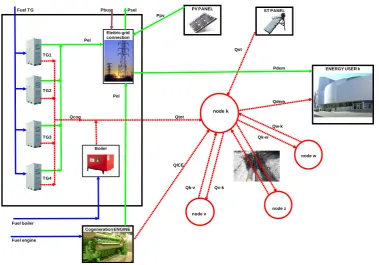
The problem cannot be solved separately for each cogeneration unit installed at a specific building because each of them is connected with the district heating network through a node where income and outcome thermal energy flows can be potentially exchanged with any other node of the network (Fig. 1). Consequently, the heat demand faced by each unit is not defined “in advance”, and the optimal operation has to be defined jointly with the optimal synthesis of the district heating micro-grids and with the number and position of CHP engines.
Figure 1. A cogeneration unit with its connections with the nodes of the district heating network.
In each time interval, the energy system is described by means of the amount of every exchanged energy flow and by two sets of binary optimization variables expressing the existence/not-existence of the components and their on/off operation. Other design binary variables and continuous operating variables can also be used to describe the district heating network to be optimized, without
Pbuy Psel Ppv
Pel
Qst TG1
Pdem
TG2
Pel
Qdem
Qcog Qtot
Qw-k
TG3 Qk-w
node w
QICE
TG4
Qk-v Qv-k
node z
Fuel boiler
Fuel engine Fuel TG
node k
node v Elettric grid
connection
Boiler
Cogeneration ENGINE
PV PANEL ST PANEL
violating the model linearity. In the following, the equations of the MILP model used in the presented optimization procedure are summarized.
The objective function is the Total Annual Cost for owning, maintaining and operating the whole system (Equation 1). The operating costs mainly consist in the sum of the sustained costs for the purchase of the external fuel energy flows, minus profits from the optional selling of electricity to another grid, for the whole year, while the owning costs are simply obtained by multiplying the total capital cost of each kind of component by the corresponding capital cost recovery factor, and the maintaining costs are regarded as proportional to the electric energy produced all the yearlong.
Variables X(j,k) represent the existence/not-existence of CHP engine (TG or ICE) “j” inside building “k”, while variables y (i,j,k) ≤ X(j,k) represent the on/off operation of the same CHP engine at the time interval “i”.
Variables r(k,v) express the existence/not-existence of the pipeline from node “v” to node “k” into the district heating network, while variables DHN (k,v) express the maximum nominal heat flow
of the same pipeline and Q(i,k,v) express the actual heat flow, sent from node “k” to node “v” through the district heating network, at the time interval “i” (Figure 1).
costTOT =
FuelCHP (i,j,k) *CFuelCHP(i) +
[Fuelboil(i,k)*CFuelboil(i) + Pbuy(i,k)*CBUY(i,k)-Psel(i,k)*CSEL(i)]+ faCHP* costCHP + faHN * costHN + faPV* costPV + faST* costST + costman
(1)
where:
costPV =
CPV*APV (k) (2)is the total capital cost of PV panels
costST =
CST*AST (k) (3)is the total capital cost of ST collectors
costCHP =
CCHP(j,k)*X(j,k) (4)is the total capital cost of CHP components
costHN =
[DHN(k,v)*E + r(k,v)*F]*l(k,v) (5)is the total capital cost of the district heating networks
costman =
Cman*Pel(i,j,k) (6)is the maintenance cost of the whole system.
The cost of each pipeline (branch) per unit length, can be considered as a linear function of the maximum nominal heat flow of the same pipeline [24], whilst the efficiency of the integration boilers can be regarded as a constant.
Note that the existence of TG, ICE and branches of the DHN are described by (binary) decision variables whilst the extensions of PV and ST panel surfaces (APV and AST, respectively) are continuous
decision variables, but none of them depend on the specific time interval. On the contrary, the on/off operation of the same components and the thermal and electrical energy flows, exchanged inside the system, are also decision variables (binary and continuous, respectively) but they can change by switching from one time interval to the next one. A first set of constraints represents the performance maps of the components which have been linearized, with negligible approximation:
FuelCHP (i,j,k) = A(j,k)*Pel(i,j,k) + B(j,k)*y(i,j,k) (7)
Qcog(i,j,k) = M(j,k)*Pel(i,j,k) + N(j,k)*y(i,j,k) (8)
Pmin(j,k)*y(i,j,k) Pel(i,j,k) Pmax(j,k)*y(i,j,k) (9)
In addition, the maximum nominal heat flow and the heat flow direction of each pipeline has to be respected:
DHN (k,v) Q(i,k,v) 0 (10)
DHNmin(k,v)*r(k,v) DHN (k,v) DHNmax(k,v)*r(k,v) (11)
r(k,v) + r(v,k) 1 (12)
The thermal demand has to be satisfied by cogeneration equipment, auxiliary boilers and solar thermal integration. At the same time the electricity demand has to be satisfied by cogeneration equipment, PV production and by electricity external purchase:
Qint(i,k) = Qdem(i,k) -
Qcog(i,j,k) + Qdiss(i,k) +
Q(i,k,v) -
Q(i,v,k) * (1-d(v,k)) - QST(i,k)(13)
Psel(i,k) =
Pel(i,j,k) – Pdem(i,k) + Pbuy(i,k) + PPV(i,k) (14)Thermal losses along the district heating network have been taken into account through constant factor , expressing the fraction of Q that is expected to be lost, per unit length:
d(v,k) = (/100)*l(v,k) (15)
The energy efficiency of both solar thermal and photovoltaic panels can be regarded as linear vs. the temperature difference between the fluid collector average temperature and the outside ambient [26, 27]:
ST = -7.5 (t-t°)/G + 0.7 (16)
PV = - 0.0009 (t°-t) + 0.1987 (17)
where t is the fluid collector average temperature, t° is the ambient temperature and G [W/m2]
is the solar radiation. Available data for G and t° have to be introduced into the model from [24]. In this case study, an average energy efficiency of solar thermal panels equal to about 42% has been obtained. Eq. 17 is valid for South oriented panels, having an inclination equal to 30° with respect to the horizontal plane.
The CO2 emissions as a result of the operation of the whole CHP and DHN can be calculated by
introducing the Carbon Intensity (CI) of fuels and purchased/sold electricity to the grid. Then, the avoided CO2 emissions can be easily calculated as the difference between the conventional and the
CHP and DHN energy production, to supply the same users.
3. Case study
The optimization model has been applied to a distributed cogeneration system with district heating, taking as a reference for the supplying of thermal energy and electricity the consumptions of six public buildings in the centre of the city of Pordenone (Italy) [28] considering this as representative of generic commercial building systems [29].
The conventional power supply, for the six buildings considered, involves an annual cost of 796,064 €/ year, for the purchase of 2959 MWh of electrical energy and for the production of 4846 MWh of thermal energy by conventional boilers, fed with natural gas [30].
analysis of the different techniques to reduce the computational effort for energy models resolution [32], including time slices and typical days or weeks identification. In [33] the approach of identifying a set of proper typical days is used in the optimal design of a multi-energy system with seasonal thermal storage, while in [34] an improved adaptive genetic algorithm is proposed to model the typical day load sequence for multi-objective optimization of a distributed generation system.
Figure 2. Plan of buildings and path of district heating network in the Pordenone city center: 1) Town Hall, 2) Theatre, 3) Library, 4) Primary school, 5) Retirement home, 6) Ex-monastery.
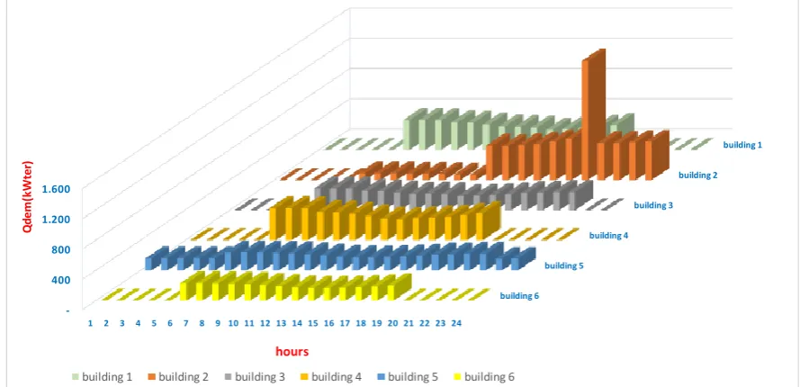
In Figures 3a and 3b, the energy demands of the 6 buildings are shown for a winter working day, as an example. In Figure 4 the total monthly energy demands are shown for all the year. Notice that the thermal demand shows strong seasonal variations, as it is common for civil buildings in the central European region.
Figure 3a. Electrical energy demand (Pdem) for a typical January working day (24 hours), for the 6 buildings considered.
Figure 3b. Thermal energy demand (Qdem) for a typical January working day (24 hours), for the 6 buildings considered.
To improve the thermal and electrical energy production, a set of thermal and photovoltaic panels can be installed on the buildings with a maximum area of 100 m2 each, except on the buildings
2 (theater) and 4 (primary school), because of their architectural constraints.
Capstone C60 has been considered as the microturbine reference model, consistently with the modular approach adopted for each local cogeneration unit (see Fig. 1) and with the characteristic of this kind of components in term of noise and pollutant emissions, which allow easily their adoption in an urban context. Full and partial load performances have been evaluated on the basis of experimental data available in literature [35]. Linear approximations have been introduced to express natural gas consumption (Fuel [kW]) and cogenerated heat (Qcog [kW]) vs. net electric power (Pel [kW]). Different electrical and thermal efficiencies of GT have been taken into account depending on the ambient temperature, varying with time inside each typical day considered.
A similar procedure has been followed to evaluate ICE performance [36], considering for the central unit a Jenbacher – GE JMS 312 GS-NL. In the ICE case, ambient temperature effect has been ignored, for reasons of simplicity. Nominal and partial load performances, at standard temperature building 1
building 2
building 3
building 4
building 5
building 6
0 100 200 300
1 2 3 4 5 6 7 8 9 10 11 12 13 14 15 16 17 18 19 20 21 22 23 24
Pd
em
(k
W
el)
hours
building 1 building 2 building 3 building 4 building 5 building 6
building 1
building 2
building 3
building 4
building 5
building 6
-400 800 1.200 1.600
1 2 3 4 5 6 7 8 9 10 11 12 13 14 15 16 17 18 19 20 21 22 23 24
Q
de
m
(k
W
te
r)
hours
conditions, are summarized in Table 1. The linear approximations of engine performance curves, in terms of energy flows, have to be regarded as adequate [10, 37, 38], without the need of introducing multi-linear approximations. Natural gas is considered as the fuel of both integration boilers and cogeneration systems. A constant thermal efficiency equal to 90% has been introduced for integration boilers, as an average value.
Figure 4. Annual distribution of energy demands for all the 6 buildings considered.
Table 1. Nominal and partial load performance of micro turbine and cogeneration ICE, at standard temperature.
Pel el th Fuel Qcog
[kW] [%] [%] [kW] [kW]
Microturbine Capstone C 60
54.9 26.2 52.2 209.5 109.4
39.9 24.2 56.4 164.9 93.0
24.8 20.0 56.7 124.0 70.3
Jenbacher – GE JMS 312 GS-NLC
601 38.9 47.4 1544 732
449 37.7 48.4 1191 576
310 37.0 49.9 838 418
A prudent value of = 10% per km has been introduced for the constant value of losses per unit length, in the district heating pipelines.
The objective function of the optimization procedure is the total annual cost for owning, maintaining and operating the whole cogeneration system, as shown in Eq. 1. This total cost depends on the cost rates of gas and electricity (sold and/or purchased) for each considered time interval, on the capital cost of cogeneration equipment and on the fixed and variable costs for pipelines in the district heating network; the values used in the calculations are shown in Table 2 and refer to the present Italian market situation.
In particular, the PV panel cost includes auxiliary and grid connection components [10], while the ST panel cost includes piping for the CHP unit integration. Cost of the fuel for boilers and cogeneration engines is different because, adopting cogeneration engines, the taxation value applied changes from civil user to industrial self-producer. All capital costs are converted into a cost rate by
0 100 200 300 400 500 600 700 800 900 1000
Jan Feb mar Apr May Jun Jul Aug Sep Oct Nov Dec
M
o
n
tl
y
d
e
m
a
n
d
[M
W
h
]
means of capital recovery factors (fa). Values equal to 0.15, 0.11 and 0.09 are used in the calculation for cogeneration engines, solar panels and district heating pipelines, respectively, to take into account the different expected life time for each kind of component (8 years for cogeneration engines, 12 years for solar panels and 16 years for pipelines).
In this case study, the total CO2 emissions are associated with the carbon intensity (CI) of both
natural gas and electricity, because they are the only input fuels at the system boundary. While the natural gas has similar CI all around the world, the electricity CI is widely variable, depending on the electricity mix of the network to which the system is connected and also on the boundary considered for the evaluation of indirect emissions [39]. In this work a value equal to 0.22 kg/kWh has been used for CI of natural gas [40, 41], while the greenhouse emissions of the electricity have been assumed equal to the specific emission factor of the main thermoelectric plant of the region where the users are located, which is a coal-fired power plant (0.79 kg/kWh) [42].
Table 2. Cost rate of electricity and capital cost of microturbines, cogeneration ICE, district heating pipelines and PV / ST panels (E and F refer to the coefficients used in Equation 5).
1st- 4thTG capital cost 65,000-100,000 [€]
ICE capital cost 500,000 [€]
PV capital cost 200 [€/m2]
ST capital cost 580 [€/m2]
Bought electric energy 0.160 [€/kWh]
Sold electric energy 0.026 -0.078 [€/kWh]
TG maintenance cost 0.010 [€/kWh]
ICE maintenance cost 0.020 [€/kWh]
Boiler fuel cost 0.56 [€/m3]
TG and ICE fuel cost 0.37 [€/m3]
Fixed cost of excavation (F) 270.63 [€/m]
Cost proportional to DHN (E) 0.179 [€/kWm]
4. Two-level optimization strategy
The objective of this project is the optimization of a complex CHP and DHN system. The proposed model is intended for district-level implementation and is concerned with the optimal layout and operation of CHP units deployed in different buildings and with the optimal configuration of heating grids connecting multiple sites in the district. The implementation of a central CHP plant and micro-CHP gas turbines distributed among the involved buildings, along with the installation of thermal collectors and photovoltaic (PV) cells, have been considered to further improve the energy efficiency and sustainability of this system, as introduced in § 2.
The original single-objective formulation of the problem was aimed at minimizing the total annual cost of ownership, maintenance and operation of the described system. To reach this objective we sought the best system configuration. This required us to identify the optimal number of CHP units and their position and the heating grid layout to minimize energy loss. Furthermore, we had to determine the optimal number of thermal collectors and PV panels for each site to satisfy energy and heating demands of each building throughout the year. The optimal solution should have also considered the environmental pollution in terms of CO2 emissions.
number of binary decision variables is low enough, as shown by the authors in [24, 25, 43, 44]. Otherwise, the computational effort becomes unacceptable. For instance, the first optimization of the case study was performed with this approach by using the commercial software FICO® Xpress
Optimization Suite [45] and a desktop computer with an Intel Core i7-4770 processor at 3.40 GHz, 16 Gb RAM and a solid-state disk. The computational time increased from a few seconds for only three buildings to 26 minutes for six buildings. This meant that the problem complexity caused by the number of the independent variables was too great to obtain a solution covering an entire town district instead of a limited number of buildings. In other words, this approach is not feasible for large scale instances. To solve problems of this kind, different approaches based on problem decomposition can be found in literature [12, 16-18]. For instance, a physical decomposition could be considered, by dividing the whole system into the heating network and the different thermal energy suppliers, but this approach is advisable if the binary variables affect only one of the sub-systems obtained by the decomposition [21].
In this case study, there are many binary variables in all sub-systems, not in only one of them, therefore a mere physically based decomposition of the problem cannot be usefully applied. To overcome this difficulty, in this study the problem has been modeled as a hierarchical problem which involves two levels: an outer and an inner level.
The outer level is concerned with the general configuration of the CHP system in terms of the number of branches of the heating grid (i.e. pipeline connections between buildings), the position of the central CHP plant, the location and the number of micro-CHP plants. The scheduling of the CHP units throughout the year, as well as the surface of thermal collectors and PV cells, are inner level variables instead. The objective of the inner level is to find the optimal operation which satisfies the constraints expressed by thermal and power demands of each final user and minimizes the operational costs of the whole system.
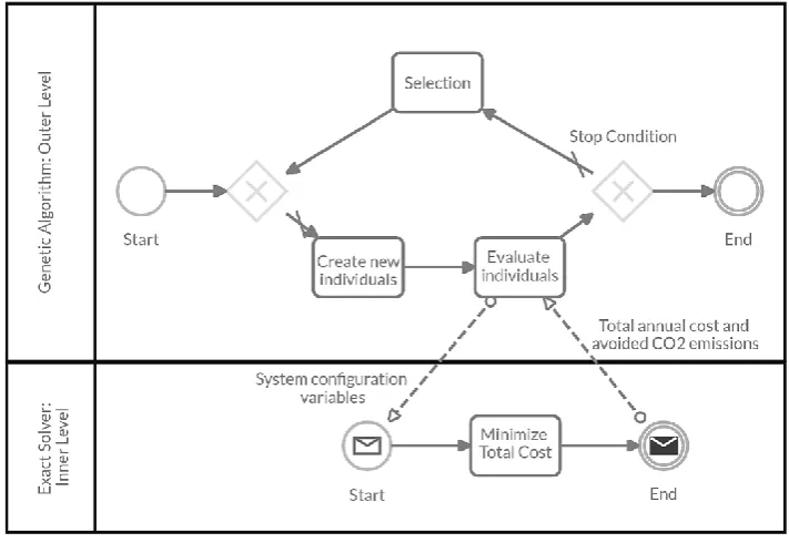
The problem has been formulated as a two-level problem with the commercial optimization software modeFRONTIER® [46], integrated with FICO® Xpress Optimization Suite. The outer level configuration has been optimized with a genetic algorithm, whereas the inner level has been solved with the Xpress exact solver.
Figure 5. Interaction of the Outer and Inner levels in the Bi-level optimization algorithm.
with 40 individuals per generation and 25 generations. The individual evaluation phase is made on the basis of the results of exact solver at the inner level. The latter receives the configuration variables of each individual and, for each of them, it performs the operation optimization using the total annual cost (CostTOT, Equation 1) as objective function. The optimal solution contains not only the minimum
total annual cost allowed by the configuration variables introduced for each individual, but also the equivalent CO2 emissions and therefore the avoided emissions, with respect to the conventional
solution for energy supply. The optimized variable assignment in the inner level is sent back to the outer level to allow the genetic algorithm to determine whether a solution is suitable for guiding the creation of the next generation of solutions, as well as the quantitative indexes of each solution (these indexes are then summarized in the Scatter Matrix and in the Probability Density Function charts, presented in the following § 5). The entire loop is repeated until the termination criterion is reached, i.e. when a further evolution of the population does not obtain any appreciable performance improvement, indicated as Stop Condition in Figure 5. It is worth noting that more than one objective function can be used to evaluate the individual performance, allowing to highlight different convergence stories and to identify the Pareto front. In this case study one second objective function (besides the total annual cost) have been considered: the avoided CO2 emissions during the year (to
be maximized), in order of measuring the environmental impact of the modeled system.
By applying this two-level approach to the case study, i.e. the optimization of the CHP system with district heating for 6 buildings, the computational times for each solution provided to the inner level were reduced to a mere 3 seconds compared to the previous 26 minutes required by the direct MILP approach. This means that we could perform 520 design evaluations in the same time without using any parallel computing functionalities of the workstation.
The modeFRONTIER® software enabled us not only to keep the original MILP model used in
the direct approach, but also to integrate it in a hierarchical optimization workflow. After an exploration of different optimization algorithms, we decided to use the genetic algorithm NSGA-II, widely discussed in literature [47]. We considered it the most suitable approach for tackling the outer level of this problem in terms of result accuracy and convergence rate. Furthermore, this approach enabled us to use the multi-core processor of the computer and thus perform in parallel multiple inner level runs, which significantly sped up the optimization process. Repeated optimization test runs resulted in the optimal problem solution in less than 15 minutes with an accurate exploration of the design space.
Given these results, a sub-set of the inner level parameters was transferred to the outer level, i.e. the surfaces of thermal collectors (AST(k)) and PV panels (APV(k)). In this way the computations at the
inner level were further streamlined without this having a negative impact on the outer level, and all design variables have been put in the outer decision level, allowing the genetic algorithm to manage directly the surfaces of thermal collectors and PV panels, in view of both objective functions.
It is worth noting that an easy implementation of the multi-objective approach has been possible because the choice of the objective as the merit function of the genetic algorithm affects only the decision variables of the outer level, not the inner level.
The presence of two objectives in the outer level and only one of those objectives, i.e. cost minimization, at the inner level, may throw the search off balance in favor of this objective. In spite of this apparent drawback, the NSGA-II algorithm is able to maintain the uniformity of the Pareto front. However, we can expect a different quality of exploration between the two tails of the front corresponding to the best values of each of the objectives. The tail of the avoided CO2 emissions
objective will be less explored, but this is not an issue because the most expensive solutions lead to a rather small additional environmental benefit in terms of CO2 emissions and has thus poor industrial
appeal.
5. Results
Figures 6 and 7 show the convergence history of the hierarchical optimization of both objectives, i.e. avoided CO2 emissions and total annual cost. In particular, Figure 6 shows that the maximum CO2
an unacceptable annual cost of 30,383,000 €/year. At this point we performed result post processing to exclude unfeasible solutions from a practical point of view. This consisted in limiting the maximum annual cost to 1,000,000 €/year. With this constraint the new optimal design has been obtained at iteration number 905 (Design ID) with 3241 t/year CO2 saving.
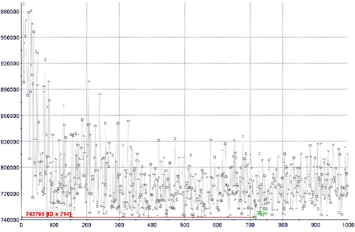
Figure 7 shows that the minimum annual cost of 742,705 €/year has been obtained at iteration number 714 (Design ID). However, the genetic algorithm had already found a value very similar to this after only about 150 iterations.
Figure 6. History of the convergence process for the objective of the avoided CO2 emissions.
Figure 7. of the convergence process for the objective of the Total annual cost.
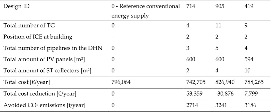
Table 3. Main results for the optimal total annual cost and for the optimal avoided CO2 emissions.
Design ID 0 - Reference conventional
energy supply
714 905 419
Total number of TG 0 4 11 9
Position of ICE at building - 2 2 2
Total number of pipelines in the DHN 0 3 5 4
Total amount of PV panels [m2] 0 600 600 594
Total amount of ST collectors [m2] 0 2 4 10
Total cost [€/year] 796,064 742,705 826,940 788,265
Total cost reduction [€/year] 0 53,359 -30,876 7,799
Avoided CO2 emissions [t/year] 0 2714 3241 3186
One of the main advantages of multi-objective optimization methods is the generation of many feasible trade-off solutions, so the designer can easily identify the best compromise. Approximately 1000 evaluations with NSGA-II have been performed in 8 minutes and a set of Pareto solutions representing equally valid CHP system configuration alternatives have been identified.
The final Pareto front obtained for the case study is shown on the Scatter Chart in Figure 8. The Cost objective (to be minimized) is plotted on the x axis whereas the avoided CO2 emissions (to be
maximized) are plotted on the y axis. The Pareto solutions, displayed as green circles, are well distributed in the design space. The reference solution is represented as a red dot at the bottom of the chart with cost value of 796,064 €/year. However, for the sake of clarity of the comparison it was placed on the x axis even though the CO2 saving is actually 0 t/year. The solution with ID 905 brings
about a CO2 saving of approximately 3241 t/year with a cost of 826,940 €/year, which is only 30,876
€/year more than the reference solution. For this reason this solution is regarded as the most environmentally friendly (see Table 3). This optimal solution includes the ICE and the maximum number of micro-gas turbine (11) and pipelines (5) among all solutions of the Pareto front.
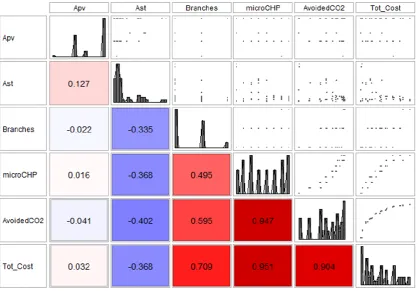
The Scatter Matrix chart available in modeFRONTIER® (Figure 9) deals in detail with the
solutions on the Pareto front and helps us understand the behavior of outer level variables, how they influence each other and how their values are distributed. The chart uses the Pearson coefficient for correlations and the Probability Density Function for variable distribution [48]. All input variables of the outer level and the two objectives are plotted on both axes: each colored square shows the strength and the type of correlation (positive or negative) between a variable pair (one plotted on the x axis and the other on the y axis).
The two objectives (total annual cost and avoided CO2 emissions) are strongly positively
correlated, as expected, but even more so with the number of micro-CHP units. It is perfectly plausible that the more the CHP components in the plant to be purchased and maintained, the higher the cost, but on the other hand this helps to reduce the CO2 emissions. These three variables (total
Figure 8. Pareto front of the multi-objective optimization.
A moderate inverse correlation can be observed between the thermal collector surface (AST) and
all the above mentioned variables. In fact, the more the branches and CHP units in the plant, the less the usefulness of the thermal collectors to satisfy the energy demand of the buildings. On the other hand, the use of solar energy implies a reduction of CHP units and therefore a lower total cost, but also less avoided CO2 emissions because additional power has to be purchased from the grid.
Figure 9. Scatter Matrix chart of the variables in the outer level
.
Reference solution cost
OB
J:
CO
2
[t
/year]
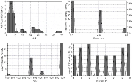
The Probability Density Function charts (Figure 10) reveal that the number of branches is in most cases limited to two mid values, i.e. 3 and 4. In no case has an optimal solution been found for the minimum (i.e. 0) and the maximum (i.e. 8) number of branches.
A significant variability can be observed in the total surface of thermal collectors AST (between 0
and 70 m2), although the majority of solutions have the lowest values. Few solar thermal collectors
are installed in all optimal solutions because of the high investment costs.
On the contrary, the PV panel range of values is quite restricted: between 590 and 600 m2, with
more than half optimal configurations having the highest value, because of the strong reduction of costs occurred in recent years for this kind of components.
Figure 10. Probability Density Function charts for the outer level variables
.
The PV panel range of values is quite restricted, i.e. between 590 and 600 m2, with more than half
optimal configurations with the highest value because of low investment costs.
Finally, we can consider the number of micro-CHP units as the most relevant outer level variable due to their rather uniform distribution on the Pareto from, as shown in Figure 10. From the Pareto front (Fig. 8) it can be noted that the solution allowing the maximum CO2 saving and, at the same
time, a reduction of the total cost compared to the reference solution, is ID 419. The main results for this compromise solution are shown in Table 3.
Once one solution has been identified in the Pareto front, the output of the optimization model contains complete information about the optimal structure and operation of the energy system. As an example, Fig. 11 shows the electricity, heat and pipelines optimal hourly schedules in 4 typical working days, for the compromise optimal solution ID 419.
Notice that the electrical and thermal energy values have been aggregated at global system level, even if the solution contains the values of all energy flows exchanged by each building and produced by each cogeneration unit. In Fig. 12 the detailed hourly schedules of heat flows through the pipelines and electric energy exchanged with the grid is shown for a typical January working day.
Looking at the heat balances, it can be noted that the cogeneration units satisfy almost the whole heat demand; in summer time the ICE is operated at partial load for about 10 hours per day and the excess heat is dissipated. The optimal solutions also contain the position of the mGTs and of the pipelines, so that the path of the micro district heating grids can be easily inferred. In particular, for the solution considered, there is only one micro district heating grid and one isolated building (Fig. 12). The purpose of the grid is to distribute the heat produced by the ICE in building 2 also to buildings 3, 4 and 6, so that a grid bifurcation is required in site 3. Building 6 is connected to the micro district heating grid, so that it can take advantage of the cogenerated heat even if there are no cogeneration units inside it.
The micro district heating grid is operated all the time, except in the summer time. This detailed information can be obtained for each identified solution and for each typical day, providing a basis for knowledge for the design of the complex energy system, taking into account in advance the peculiarities of its optimal management.
6. Conclusions
The design and operation optimization of integrated multi-component energy systems generally require a binary variable set to be introduced to describe the existence/absence and the on/off operation status of components and energy connections inside the model. Besides these, other continuous variables have to be introduced for modelling the energy and material flows exchanged among components, as well as other possible design options. In these kinds of optimization problems the decomposition approach, often suggested in literature [13, 17, 18], may be not best suited, because the discontinuous nature of variables present in many sub-problems can prevent the convergence of the whole problem.
In the case study there are many binary variables in all sub-systems. It is a distributed cogeneration and district heating system, including a set of micro-cogeneration gas turbines (to be located at the energy user sites), a centralized cogeneration system, photovoltaic panels, solar thermal collectors and various district heating pipelines, potentially connecting the users. The existence of each one of these components is related to a binary variable in the optimization problem.
In this paper an innovative approach is presented that allows to exploit the essential positive characteristics of decomposition, overcoming its difficulties by using a bi-level optimization strategy, which involves an outer and an inner level. The outer level configuration was optimized with a genetic algorithm of the commercial optimization software modeFRONTIER®, whereas the inner
level was solved with FICO® Xpress Optimization Suite. The outer is concerned with all the structural
variables of the whole system, including the distribution of the micro CHP units, at the energy user sites, the district heating pipelines of the network and the surface of thermal collectors and PV panels, leaving at the inner level only the MILP problem of the optimal operation of the whole system. In this approach, a multi objective optimization can be easily performed, by introducing a second objective in the outer level only, and the Pareto front can be obtained. The avoided CO2 emissions
have been introduced as a second, environmental objective, besides the minimum annual cost. Anyhow, the solutions obtained confirm that CHP systems, optimized for the minimum annual cost, can be favorable from both the economic and environmental standpoints. In the case study, the minimum cost solution allows a monetary saving of about 53,000 €/year and a CO2 saving of about
2700 t/year. A possible environmental-friendly alternative on the Pareto front allows a maximum CO2 saving of about 3240 t/year, with an additional cost of only 31,000 €/year, compared to the conventional solution.
Figure 11.Global electricity, heat and pipelines hourly schedules in 4 typical working days, for the compromise
optimal solution ID 419. 0 200 400 600 800 1.000 1.200 1.400
1 2 4 5 6 7 8 9 10 11 12 13 14 15 16 17 18 19 20 21 22 23 24
E lec tr ic a l[ k W e] hours
Electrical energy balance for a typical January working day
pel pelbig pbuy Ppv RICel
0 200 400 600 800 1.000 1.200 1.400
1 2 3 4 5 6 7 8 9 10 11 12 13 14 15 16 17 18 19 20 21 22 23 24
El ec tr ic al [k W e] hours
Electrical energy balance for a typical March working day
pel pelbig pbuy Ppv RICel
0 200 400 600 800 1.000 1.200 1.400 1.600 1.800 2.000 2.200
1 2 3 5 6 7 8 9 10 11 12 13 14 15 16 17 18 19 20 21 22 23 24
T h er ma l[ k W t] hours
Thermal energy balance for a typical January working day
pter pterbig ptin Pst RICTer
0 200 400 600 800 1.000 1.200 1.400 1.600 1.800 2.000 2.200
1 2 3 4 5 6 7 8 9 10 11 12 13 14 15 16 17 18 19 20 21 22 23 24
Th er ma l[ kW t] hours
Thermal energy balance for a typical March working day
pter pterbig ptin Pst RICTer
0 100 200 300 400 500 600 700
1 2 3 4 5 6 7 8 9 10 11 12 13 14 15 16 17 18 19 20 21 22 23 24
He at fl ow p ip el in e[ kW t] hours
Heat flow of the pipeline [node V-k] for a typical January working day
edif 2- node 3 edif 3- node 4 edif 3- node 6 edif 5- node 6
0 100 200 300 400 500 600 700
1 2 3 4 5 6 7 8 9 10 11 12 13 14 15 16 17 18 19 20 21 22 23 24
H ea t flo w p ip eli n e[ kW t] hours
Heat flow of the pipeline[node V-K] for a typical March working day
edif 2- node 3 edif 3- node 4 edif 3- node 6 edif 5- node 6
0 200 400 600 800 1.000 1.200 1.400
1 2 3 4 5 6 7 8 9 10 11 12 13 14 15 16 17 18 19 20 21 22 23 24
El ec tr ic al [k W e] hours
Electrical energy balance for a typical June working day
pel pelbig pbuy Ppv RICel
0 200 400 600 800 1.000 1.200 1.400
1 2 3 4 5 6 7 8 9 10 11 12 13 14 15 16 17 18 19 20 21 22 23 24
El ec tr ic al [k W e] hours
Electrical energy balance for a typical November working day
pel pelbig pbuy Ppv RICel
0 200 400 600 800 1.000 1.200 1.400 1.600 1.800 2.000 2.200
1 2 3 4 5 6 7 8 9 10 11 12 13 14 15 16 17 18 19 20 21 22 23 24
Th er ma l[ kW t] hours
Thermal energy balance for a typical June working day
pter pterbig ptin Pst RICTer
0 200 400 600 800 1.000 1.200 1.400 1.600 1.800 2.000 2.200
1 2 3 4 5 6 7 8 9 10 11 12 13 14 15 16 17 18 19 20 21 22 23 24
Th er ma l[ kW t] hours
Thermal energy balance for a typical November working day
pter pterbig ptin Pst RICTer
0 100 200 300 400 500 600 700
1 2 3 4 5 6 7 8 9 10 11 12 13 14 15 16 17 18 19 20 21 22 23 24
H ea t fl o w p ip el in e[ kW t] hours
Heat flow of the pipeline [node V-k] for a typical June working day
edif 2- node 3 edif 3- node 4 edif 3- node 6 edif 5- node 6
0 100 200 300 400 500 600 700
1 2 3 4 5 6 7 8 9 10 11 12 13 14 15 16 17 18 19 20 21 22 23 24
H ea t fl o w p ip eli n e [k W t] hours
Heat flow of the pipeline [node V-k] for a typical November working day
Figure 12.Detailed hourly schedules of heat flows in the pipelines and electric energy exchanged with the grid,
in a typical January working day, for the compromise optimal solution ID 419.
From the data analysis, it can be observed that the evolutionary strategy, implemented in the outer optimization level, allows us to obtain a value very close to the actual optimum after a limited number of iterations. The two objectives are strongly positively correlated and they are mostly influenced (even though to different extents) mainly by the number of micro CHPs, and also by the number of pipelines in the district heating network. This fact highlights how the dislocation of the CHP units is the most critical choice, in order to really obtain the economic and environmental advantages which are expected by the cogeneration technology.
In addition, detailed information can be obtained for each identified solution and for each typical day, providing a knowledge basis for the design of the complex energy system, taking into account in advance the peculiarities of its optimal management.
In summary, the proposed method allows the simultaneous optimization of the distributed cogeneration system and the configuration of micro-district heating networks with multiple users, with an innovative approach, applicable to complex systems, allowing a significant reduction of computing time thanks to the proposed two-level optimization procedure.
Nomenclature
A, ..,L generic coefficients of linear approximation [consistent dim.];
APV PVpanel surface [m2];
AST STpanel surface [m2];
costCHP capital cost of CHP system [€];
costHN total capital cost of district heating network [€];
costman maintenance cost [€/year];
costPV total capital cost of PV panels [€];
costST total capital cost of ST panels [€];
costTOT owning, maintaining and operating total costs [€/year];
C specific cost [€/kW];
ICE
TG
TG
TG TG
5
6
3
2
CI carbon intensity [kg/kWh];
d(v,k) thermal losses fraction along the district heating pipeline from node v to node k; DHN nominal heat flow of a district heating pipeline [kW];
E cost coefficient of the DHN proportional to DHN [€/Kw m];
fa capital cost recovery factor [year-1];
F fixed cost coefficient of the DHN [€/m]; Fuelboil fuel for integration boiler [kW];
FuelCHP fuel for CHP system [kW];
G solar radiation [W/m2];
l(v,k) length of the pipeline district heating from node v to k [m];
P power
Pbuy purchased electrical energy [kW]; Pdem electrical energy demand [kW];
Pel cogenerated electrical energy [kW];
Psel sold electrical energy by CHP system [kW];
Q generic heat flow inside the district heating network [kW];
QST heat flow produced by solar thermal panels [kW];
Qcog cogenerated thermal energy [kW];
Qdem thermal energy demand [kW]; Qdiss dissipated thermal energy [kW];
Qint thermal integration [kW];
t fluid collector average temperature [°C];
t° ambient temperature [°C]; X, y, r generic binary variables;
Acronyms
CHP Combined Heat and Power;
CHCP Combined Heat, Cooling and Power; DHN District Heating Network;
HN Heating Network;
ICE Internal Combustion Engine;
MILE Mixed Integer Linear Exergoeconomic; MINLP Mixed Integer Non-Linear Programming;
MILP Mixed Integer Linear Programming; OBJ Objective function;
PV Photovoltaic;
ST Solar thermal; TG Gas Turbine;
Greek symbols
percentage thermal losses along district heating pipeline per unit length [km-1];
efficiency;
th thermal;
i generic time interval; j generic CHP system;
k generic building or node;
v, w, z generic node of the district heating network;
References
1. H. Lund, B. Moller, B.V. Mathiesen, A. Dyrelund, The role of district heating in future renewable energy
systems, Energy2010, 35, 1381–1390.
2. S. Kelly, M. Pollitt, An assessment of the present and future opportunities for combined heat and power
with district heating (CHP-DH) in the United Kingdom, Energy Policy2010, 38, 6936–45.
3. B. Rezaie, M.A. Rosen, District heating and cooling: review of technology and Potential enhancements,
Applied Energy2012, 93, 2–10.
4. A. Lake, B. Rezaie, S. Beyerlein, Review of district heating and cooling systems for a sustainable future,
Renewable and Sustainable Energy Reviews2017, 67, 417–425.
5. J. A. Fonseca, T. Nguyen, A. Schlueter, F. Marechal, City Energy Analyst (CEA): Integrated framework for
analysis and optimization of building energy systems in neighborhoods and city districts, Energy and
Buildings2016, 113, 202–226.
6. M.A. Lozano, J.C. Ramos, M. Carvalho M, L. Serra, Structure optimization of energy supply systems in
tertiary sector buildings, Energy and Buildings2009, 41, 1063-1065.
7. H. Wang, W. Yin, E. Abdollahi, R. Lahdelma, W. Jiao, Modelling and optimization of CHP based district
heating system with renewable energy production and energy storage, Applied Energy2015, 159, 401-421.
8. A. Bischi, L. Taccari, E. Martelli. E. Amaldi, G. Manzolini, P. Silva, S. Campanari, E. Macchi, A detailed
MILP optimization model for combined cooling, heat and power system operation planning, Energy2014,
74, 12-26.
9. A. Reverberi, A. Del Borghi, V. Dovì, Optimal design of cogeneration systems in industrial plants combined
with district heating/cooling and underground thermal energy storage, Energies, 2011, 4, 2151-2165.
10. M.A. Lozano, Planteamiento optimo de sistemas de cogeneración (in Spanish). Proceedings of the 2nd
Congreso Iberoamericano de Ingeniería Mecánica, Belo Horizonte (Brazil),december 12-15 1995.
11. D. Buoro, M. Casisi, P. Pinamonti, M. Reini, Optimization of distributed trigeneration system integrated
with district heating and cooling micro-grids, Distributed generation and alternative energy journal2011, 26,
7–33.
12. C.A. Frangopoulos, M. R. von Spakovsky, E. Sciubba, A Brief Review of Methods for the Design and
Synthesis Optimization of Energy Systems, International Journal of Applied Thermodynamics2002, 5, 151-160.
13. L.F. Fuentes-Cortès, A.Flores-Tlacuahuac, Integration of distributed generation technologies on suitable
buildings, Applied Energy2018, 224, 582-601.
14. X. Zheng, G. Wu, Y. Qiu, X. Zhan, N. Shah, N. Li, Y. Zhao, A MINLP multi-objective optimization model
for operational planning of a case study CCHP system in urban China, Applied Energy2018, 210, 1126–1140.
15. J.F. Marquanta, R. Evinsa, L.A. Bollingera, J. Carmelietb, A holarchic approach for multi-scale distributed
energy system optimization, Applied Energy2017, 208, 935–953.
16. J.R. Muñoz, M.R. von Spakovsky, A Decomposition Approach for the Large Scale Synthesis/Design
Optimization of Highly Coupled, Highly Dynamic Energy Systems, International Journal of Applied Thermodynamics 4 (2001) 19-33.
17. J.R. Muñoz, M.R. von Spakovsky, The Application of Decomposition to the Large Scale Synthesis/Design
Optimization of Aircraft Energy Systems, International Journal of Applied Thermodynamics2001, 4, 61-76.
18. B. Oyarzabal, M.R. von Spakovsky, W. Ellis, Optimal Synthesis/Design of a PEM Fuel Cell Cogeneration
System for Multi-Unit Residential Applications–Application of a Decomposition Strategy, Journal of Energy
Resources Technology2004, 126, 30-39.
19. C. A. Frangopoulos, Thermoeconomic Functional Analysis and Optimization, Energy1987, 7 563-571.
20. M.R. von Spakovsky, R.B. Evans, The Optimal Design and Performance of Thermal System and their Components,
In Analysis and Design of Advanced Energy System Fundamentals, A.E.S. vol.3-1, A.S.M.E. ed. N.Y (USA), 1987,
21. M. Reini, D. Buoro, Mixed Integer Linearized Exergoeconomic (MILE) method for energy system synthesis and optimization, Proceedings of the 23th International Conference on Efficiency, Cost, Optimization, Simulation and Environmental Impact of Energy Systems - ECOS 2010, , Lausanne (CH),June 14-17 2010.
22. K. Ito, S. Akagi, An optimal planning method for a marine heat and power generation plant by considering
its operational problem, International Journal of Energy Research1986, 10, 75-85.
23. R. Yokoyama, K. Ito, K. Kamimura, F. Miyasaja, Development of a General purpose optimal operational
planning system for energy supply plants, Journal of Energy Resources Technology1994, 116 290-296.
24. M. Casisi, P. Pinamonti, M. Reini, Optimal lay-out and operation of CHP distributed generation systems,
Energy2009, 34, 2175-2183.
25. M. Casisi, A. De Nardi, P. Pinamonti, M. Reini, Effect of different economic support policies on the optimal
synthesis and operation of a distributed energy supply system with renewable energy sources for an
industrial area, Energy Conversion and Management2015, 95, 131-139.
26. B.Y.H. Liu, R.C. Jordan, The long-term average performance of flat-plat solar energy collectors, Solar Energy
1963, 7, 53-74.
27. IFA–CNR, Climate data of the Italian Energy Finalized Project (Progetto Finalizzato Energetica), 1979 (in
Italian).
28. G. Di Prampero, Technical-economic comparison between distributed generation and DH for a
cogeneration urban system, Bachelor Thesis, University of Trieste, Italy, 2005 (in Italian).
29. M. Medrano, J. Brouwer, V. McDonell, J. Mauzey, S. Samuelsen, Integration of distributed generation
systems into generic types of commercial buildings in California, Energy and Buildings2008, 40 537–548.
30. M. Casisi, L. Castelli, P. Pinamonti, M. Reini, Effect of different economic support policies on the optimal
definition and operation of a CHP and RES distributed generation systems, Proceedings of the ASME TURBO EXPO 2008, Berlin (D), June 9-13 2008.
31. M. Ameri, Z. Besharati, Optimal design and operation of district heating and cooling networks with CCHP
systems in a residential complex, Energy and Buildings2016, 110, 135–148.
32. S. Pfenninger, Dealing with multiple decades of hourly wind and PV time series in energy models: A
comparison of methods to reduce time resolution and the planning implications of inter-annual variability,
Applied Energy2015, 152, 83-93.
33. P. Gabrielli, M. Gazzani, E Martelli, M.Mazzotti, Optimal design of multi-energy systems with seasonal
storage, Applied Energy2018, 219, 408–424.
34. Y. Gao, J. Liu, J. Yang, H. Liang, J. Zhang, Multi-objective of multi-type distributed generation considering
timing characteristics and environmental benefits, Energies2014, 7, 6242-6257.
35. Greenhouse Gas Technology Center – Southern Research Institute, Environmental Technology Verification
Report - Combined Heat and Power at a Commercial Supermarket - Capstone 60 kW Microturbine CHP System, Report SRI/USEPA-GHG-VR-27, Sept. 2003.
36. Jenbacher , GE Technical description of cogeneration plant, JMS 312 GS-NLC.
37. S. Consonni, G. Lozza, E. Macchi, Optimization of a cogeneration systems operation Part A: Prime movers
modelization, Proceedings of ASME Cogen-Turbo ’89, Nice (F), august 30 – September 1 1989
38. M. Reini, R. Taccani, A. Giadrossi, Optimal Operation of a Diesel Engine Cogeneration System Including
Thermal and Mechanical Energy Storage, Proc. of ECOS 2001, A. Ozturk and Y. A. Gogus eds., Istanbul (Turkey), July 4-6 2001.
39. L. Ji et al., Greenhouse gas emission factors of purchased electricity from interconnected grids, Applied
Energy2016, 184, 751-758.
40. Eurostat, Environment, transport and energy indicators, ISSN-1725-4566; Eurostat Pocketbooks 2009,
http://epp.eurostat.ec.europa.eu/ .
41. IPCC Guidelines 2006, Revised 1996 IPCC Guidelines for National Greenhouse Gas Inventories – Reference
manual.
42. ENDESA Italia, Sustainability Report 2003 (In Italian).
43. D. Buoro, P. Pinamonti, M. Reini, Optimization of a Distributed Cogeneration System with solar district
heating, Applied Energy2014, 124, 298-308.
44. D. Buoro , M. Casisi, A. De Nardi, P.Pinamonti, M. Reini, Multicriteria Optimization of a Distributed
Energy Supply System for an Industrial Area, Energy2013, 58, 128-137.
47. K. Deb, A. Pratap, S. Agarwal, T. Meyarivan, A fast and elitist multiobjective genetic algorithm: NSGA-II,