http://www.sciencepublishinggroup.com/j/ajnna doi: 10.11648/j.ajnna.20190501.13
ISSN: 2469-7400 (Print); ISSN: 2469-7419 (Online)
Robust Minimal Spanning Tree Using Intuitionistic Fuzzy
C-means Clustering Algorithm for Breast Cancer Detection
Nithya
1, Bhuvaneswari
1, Senthil
2, *1
Department of Mathematics, Mother Teresa Women’s University, Kodaikanal, India
2District Rural Development Agency, Dindigul, India
Email address:
*
Corresponding author
To cite this article:
Nithya, Bhuvaneswari, Senthil. Robust Minimal Spanning Tree Using Intuitionistic Fuzzy C-means Clustering Algorithm for Breast Cancer Detection. American Journal of Neural Networks and Applications. Vol. 5, No. 1, 2019, pp. 12-22. doi: 10.11648/j.ajnna.20190501.13 Received: May 10, 2019; Accepted: June 10, 2019; Published: June 29, 2019
Abstract:
Breast cancer is the most common cause of death in women and the second leading cause of cancer deaths worldwide. Primary prevention in the early stages of the disease becomes complex as the causes remain almost unknown. However, some typical signatures of this disease, such as lumps and microcalcifications appearing on mammograms, can be used to improve early diagnostic techniques, which is critical for womens quality of life. X-ray mammography is the main test used for screening and early diagnosis, and its analysis and processing are the keys to improving breast cancer prognosis. In this paper, we have presented a novel approach to identify the presence of breast cancer lumps in mammograms. The proposed algorithm for selecting initial cluster centers on the basis of minimal spanning tree (MST) is presented. MST initialization method for the intuitionistic fuzzy c-means clustering algorithm for clear to identify of abnormalities for mammography images and Breast cancer patients symptoms used to predictive probability calculated by Pearson Chi-Square (χ2) test at 0.05 significance level indicate a highly significant correlation between mammography performance and clinical symptoms of breast cancer. Our findings suggest that mammography is highly efficient and promising technique.Keywords: Breast Cancer, Mammograms, Intuitionistic Fuzzy C-means, Initial Cluster Center, Minimum Spanning Tree,
Partition Coefficient, Validation Function1. Introduction
Breast cancer is characterized by uncontrolled growth of epithelial cells with an acquired ability of local invasion and distant metastatic dissemination. Morphology and distinctive clinical presentation of breast cancer among patients is highly diversified because of heterogeneity acquired due to distinct mutations, diverse sub population of stem cell and heterotypic signaling between parenchymal and stromal cells within tumor microenvironment. The biggest problem in medical science includes the diagnosis of disease since the reason of breast cancer is unknown, although scientists know some of the risk factors like ageing, genetic risk factors, family history, menstrual periods, not having children, obesity, alcohol, overweight, etc. [1-2, 4]. Symptoms of cancer include a lump in the breast or underarm that persists after menstrual cycle, swelling in the armpit, pain or tenderness in the breast, any change in the size, contour, texture, or temperature of the
mechanism practiced for detection of breast cancer. World
Health Organization (WHO) recommends use of
mammography testing as vital part early diagnostic procedures to reduce the mortality rate. Three fold decrease in mortality rate of breast cancer has been reported in developed countries by practicing mammography in early detection of cancerous lumps in breast [7]. High mortality rate of breast cancer in Pakistan is due to the poverty, lack of awareness about cancer and its detection methods and high cost as well as fear of mammography testing and other diagnostic procedures [8-9]. Studies on intuitionistic fuzzy set are done by Atanassov on theory and application [10]. Zhang and Chen, suggested a clustering approach where an intuitionistic fuzzy similarity matrix is transformed to interval valued fuzzy martrix [11]. Chaira, recently proposed a novel intuitionistic fuzzy c-means (IFCM) algorithm using intuitionistic fuzzy set theory [12]. IFCM has two serious shortcomings, Firstly, it easily falls into local minima, Secondly, it is necessary to specify the number of clusters and the algorithm is very sensitive to the initial center [13-14]. The graph data structure is being considered as a suitable mathematical tool to model the inherent relationship among data. Reddy, proposed an MST-based cluster initialization for k-means which bridges the k-means and the MST-based clustering algorithms [15]. Huang etal, used the Kruskal algorithm to generate the MST of all data points and then deletes k-1 edges according to the order of their weights [16]. In summary, selecting proper initial cluster centers is an NP problem, and numerous improved methods have not yet been widely applied [11]. Therefore, the selection of initial cluster centers requires further research.
In order to diagnose breast cancer, there are currently four main methods used to distinguish benign lumps from malignant ones: surgical biopsy, mammography, magnetic resonance imaging and fine needle aspiration with visual interpretation. Fine needle aspiration of breast masses is non-traumatic, and mostly invasive diagnostic test that obtains information needed for evaluate of malignancy. Objective of current study was to provide an insight in better diagnosis of breast cancer through statistical evaluation of sensitivity, specificity, predictive accuracy and probability of mammography based breast tumor detection.
Minimum spanning tree is a useful graph for detecting clusters of a given set of data points. MST has been well suited for clustering in the field of pattern recognition, image processing and computational biology. In this paper is presented a novel approach to automatically detect the breast cancer. The proposed approach utilizes initialization method based on MST is proposed to compute initial cluster centers for the Intuitionistic fuzzy c-means clustering algorithm for clear to identify of abnormalities for mammography images. We summarized the mammography results and evaluated the accuracy of mammography, specificity, sensitivity, positive likelihood ratio, negative likelihood ratios were initially calculated. In addition to all these performance evaluation measures, predictive probability of mammography screening was also evaluated through Pearson chi square analysis.
2. Quantitative Analysis of
Mammograms
For 60 highly suspicious cases mammography were obtained in which area of lump was highlighted and specificity and sensitivity parameters were calculated. Calculations include total number of true positive (TP), true negative (TN), false negative (FN) and false positive (FP) cases were calculated. among these four classified categories True negative patients were those women in which no lump was identified and symptoms were due to normal breast cycle or clotting of fatty tissues were present. False positive (FP) were those with benign cancer while TP were cases in which malignant or invasive breast cancer was detected. False negatives cases where those who developed malignant breast cancer during the period of screening (12 months). Age of presentation of disease symptoms and mammography screening was also recorded. Predictive probability of breast cancer detection based on mammography screening is examined using chi square test χ2 test at ≤0.05 significance level. Along with this percentage distribution of 60 selected cases based on obvious breast cancer clinical symptoms was also calculated shown in Table 11.
2.1. Sensitivity
The sensitivity is expressed as the ratio of number of true positive, to the sum of ratio of false negative and true positive. Purpose of calculating sensitivity is to measure the reliability of a diagnostic system at making positive and negative identification. Hence to calculate sensitivity for our system understudy, we applied following formula.
Sensitivity TP 100
TP FN
= ×
+
2.2. Specificity
Specificity is expressed as the ratio of the number of true negatives, to the sum of false positive and true negative. This value defines the probability of a screening test to identify true negative cases.
Specificity TN 100
TN FP
= ×
+
2.3. Positive and Negative Likelihood Ratio Calculation
In the next step, sensitivity and specificity values are used to calculate positive likelihood ratio and negative likelihood ratio. These calculations will further measure the accuracy of mammography based breast cancer detection. Statistical formula used for calculating positive and negative likelihood ratios based on our study sample is given below:
Positive Likelihood Ratio =
(
)
1
Sensitivity Specificity
Negative Likelihood Ratio =
(
1 Sensitivity)
Specificty
−
2.4. Predictive Probability
Predictive probability of first screen mammography in accurate detection of breast lumps is calculated through chi square (χ2 ) at < 0.05 level of significance. Chi square
(χ2)formula given below where O denotes observed values of TP, TN, FP and FN cases given in Table 12 and E denotes expected values calculated in Table 14.
Chi-square (χ2)
2 (O E)
E
− =
∑
3. Minimal Spanning Tree Algorithm
In this section, we proposed Canberra distance measures for construct the minimal spanning tree.
3.1. Canberra Distance Measure MST
Given the grayscale point set D, the hierarchical methods starts by constructing a minimal spanning tree (MST) from the points in D. In x=( ,x x1 2,...xn)T and
1 2
( , ,... n)T
y= y y y are two points of a MST and ( , )e x y is an edge between x and y then the Canberra distance between x and y is denoted by ( , )d x y and calculated using equation (1) [17],
1 1 ( , )
n i i i i i
x y d x y
K x y
= − =
+
∑
(1)where K be the number of non-zero pairs.
3.2. Cluster Separation (CS)
The definition of CS between cluster centers is given by the following:
min
max
E CS
E
= (2)
where Emax is the maximum length edge in the MST, which represents two centroids that are at maximum separation and
min
E is the length edge in the MST, which represents two centroids that are nearest to each other. Then the CS represents the relative separation of the centroids. The value of CS ranges from 0 to 1. A low value of CS means that the two centroids are too close to each other and the corresponding MST Separation not valid. A high CS value means the MST separation of the data is even and valid. If the CS is greater than the threshold, the MST partition of the dataset is valid. Then, we increase the number of cluster by and test the CS again. This process continuous until the CS is smaller than the threshold. The value setting of the threshold for the CS will be practical and is dependent on the dataset. The higher the value
of the threshold the smaller the number of clusters would be, generally the value of the threshold will be ≻0.8.
3.3. Algorithm for Determining the Initial Cluster Centers
Algorithm: GMST Input: Data points
Output: optimal number of cluster centers
Let e1 be an edge in the CMST1 constructed from data points Let e2 be an edge in the CMST2 constructed from C. Let STbe the set of disjoint subtrees of CMST1.
1. Create a node v, for each data points. 2. Compute the edge weight using equation (1). 3. Construct an CMST1 from 2.
4. ST =ϕ , nc=1 ,C=ϕ. 5. Repeat.
6. For eache1∈CMST1.
7. Current longest edge e remove e1 from GMST1. 8. ST =ST∪{ }/ /T' T'is new disjoint subtrees(regions). 9. nc=nc+1.
10.Compute the center c of Ti iusing average of points.
11. { }
i
T T i
C=∪ ∈S c .
12.Compute the edge weight using equation (3.3). 13.Construct a GMST2 T from C.
14.Emin=get-min length edge. 15.Emax=get-max length edge.
16. min
max
E CS
E
= .
17.Until CS<0.8.
18.Merge the closest neighbour from GMST2.
19.Update the clusters points, repeat step 12 to step 18. 20.Finally we obtain the cluster centers.
4. Formulation of Proposed Kernel
Function Induced IFCM Based on
Gaussian Function
4.1. Intuitionistic Fuzzy C-means (IFCM) Algorithm
Intuitionistic fuzzy set given by Atanassov [3] considers both membership µ( ),x x∈X and non-membership
( ),x x X
ν ∈ . An intuitionistic fuzzy set A in X, is written as
{
, A( ), A( ) \}
A= x µ x ν x x∈X
where µA( )x →[ 0,1],νA( )x →[ 0,1] are the membership and non-membership degrees of an element in the set A with the condition 0≤µA( )x +νA( )x ≤1when νA( )x = −1 µA( )x
for every x in the set A, then the set A becomes a fuzzy set. Also indicated a hesitation degree, πA( )x which arises due to lack of knowledge in defining the membership degree of each element x in the set A and is given by
( ) 1 ( ) ( )
A x A x A x
In [5] intuitionistic fuzzy c-means, minimizes the objective function as:
∞
∑
∑
∑
u x c + π e 1<m<=
J 1 πi
C 1 i i 2 k i C 1 = i N 1 = k m ik
IFCM (3)
ik ik ik
u ∗=u +π , where uik∗ denotes the intuitionistic fuzzy membership and: 2 1 1 1 ik m c i k i j j u x c x c − = = − −
∑
(4)1
1 (1 ) , 0
ik uik uikα α
π = − − − α > (5)
1 1 N m ik i i k N m ik i u x c u = = =
∑
∑
(6)1 1 N i ik k N π∗ π =
=
∑
(7)This iteration will stop when:
{
1}
maxij uik∗ +k −uik∗k <∈
where ∈ is a termination criterion between 0 and 1, whereas k is the iteration steps. This procedure converges to a local minimum or a saddle point of JIFCM .
4.2. Kernel Function Induced IFCM Algorithm
The function K x y( , )is called a kernel function and we assume this known function, as Gaussian radial basis function:
2 2
( , ) c
x y
K x y e σ − −
=
This paper proposes an efficient weighted MST based IFCM by introducing kernel function that allows the clustering of objects to be more reasonable. The modified proposed objective function is given by:
2
1
1 1 1
( ) ( ) i , 1
C N C
m
IFCM ik k i i
i k i
J u ∗ ϕ x ϕ v π∗e−π∗ m
= = −
=
∑∑
− +∑
< < ∞ (8)where ϕ stands as map and the distance function can be expressed using in product space as:
) v ( ), x ( 2 ) v ( ), v ( ) x ( ), x ( ) v ( ) x ( i k i i k k 2 i k φ φ φ φ + φ φ = φ φ
To obtain kernel induced IFCM based Gaussian function the distance function can be modified as:
2
(xk) ( )vi G x x( k, k) G v v( , ) 2 (i i G x vk, )i
ϕ −ϕ = + −
where k=1, 2, 3...N and i=1, 2, 3...C.
Let us expressG x v( k, )i , between pixel xk and vi as the
product of a feature similarity term and spatial proximity term:
2 2
2 2
( ) ( )
( , ) exp exp
2 2
k i k i
k i
X I
x v I x I v
G x v
σ σ − − − − = ∗ (9)
where σ is a parameter which can be adjusted by users.
Using the above expression we obtain G x x( k, k)=1 and G v v( , )i i =1 , so the distance function can be rewritten as:
2
(xk) ( )vi 2 (1 G x v( k, ))i
ϕ −ϕ = − (10)
Substituting & we get kernel induced MST based IFCM is given by:
∞ m 1 e ) ) v , x ( G 1 ( u 2
J C 1 i
1 i i C 1 i N 1
k k i
m ik
IFCM = ∑ ∑ +∑π π < <
= = (11)
4.3. Obtaining Membership
To obtain equation for calculating membership we minimizing the objective function:
∞
m 1 e
∑ ∑ ∑u (1 G(x ,v))
2
J C 1 i
1 i i C 1 i N 1
k k i
m ik
IFCM= + π π < <
= = (12)
Therefore, the above objective function (6) can be minimized using one Lagrangian multiplier:
1
1 1 1
*
1
2 (1 ( , ) )
1 ,
i
C N C
m
IFCM ik k i i
i k i
C ik i
J u G x v e
u π π λ ∗ − ∗ ∗ = = − = = − + − −
∑∑
∑
∑
whereλ is a Lagrange multiplier.
To adjust uik&vifor minimum Jm , we set to zero the
derivative of JIFCM( , , )U V λ with respect touik for m≻1 .
* 1
* 2 1 ( 0
m IFCM
ik k i
ik
J
mu G x v
u λ − ∂ = − − − = ∂
(
)
1 1* 1 1
1 ( , )
m m
ik k i
m
u =λ − G x v −
−
To calculateλ, Substitute the above u*ik in the identity constraint for all values of k, we get following relation,
*
1
2 ( ) 0
N m m
ik k i
i k
J
u x v
v =
∂
= − − =
∂
∑
The minimum of JIFCM with respect to viwas computed
by taking the partial derivative of JIFCM equal to zero.
1 1 1 1 1 1 1
(1 ( , ))
m
C m
k i i
m
G x v
λ − − = = −
∑
So that vi and u*ikcan be calculated by the relation,
we obtain: * 1 1 1 1
1 ( , )
1 ( , )
ik C
k i m k j j
u
G x v G x v
− = = − −
∑
(13)* 1 * 1 ( ) ( , ) ( ) ( , ) N m
ik k i k
k
i N
m
ik k i
k
u G x v x
v
u G x v
=
=
=
∑
∑
(14)The MST based FCM algorithm iteratively optimizes
IFCM
J by continuous updating u*ik and vi until the
difference in successive u*ikvalues is very small≤ ∈, where
∈is a small positive value between 0 and 1.
5. Efficient Kernel Induced IFCM Based
on Gaussian Function [KIFCM]
5.1. Efficient KFCM Algorithm
Stage 1: Set the cluster centroids
{ }
1c i i
v = by using Canberra
MST initialization method.
Stage 2: Compute the membership function using (13).
Stage 3: Update the cluster centroids using (14).
Stage 4: Estimate objective function using (12).
Stage 5: Go to stage (2)-(3), repeat until convergence. The termination criterion is as follows Jm−Jm−1 ≺∈ where m is the iteration count, ∈ is a small number that can be set by the user.
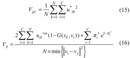
5.2. Validation Function Based on Feature Structures
Two representative functions for the fuzzy partition namely; Partition coefficient Vpc and Validation function Vp
are used to evaluate the validity of clustering [18-19].
* 2
1 1
1 N C
pc ik
k i
V u
N = =
=
∑∑
(15){
}
1
1 1 1
2
2 (1 ( , ) )
min
i
C N C
m
ik k i i
i k i
p
i j
u G x v e
V
N v v
π π − ∗ ∗ ∗ = = − − + = × −
∑∑
∑
(16)The proposed efficient weighted MST obtained cluster centers; the KIFCM algorithm continues iteratively updates, membership and centroids with these values. When this improved, Efficient KIFCM algorithm has converged, another defuzzification process takes place in order to convert the fuzzy partition matrix to a crisp partition matrix that is segmented.
6. Results and Discussion
This section describes some experimental results on random data, corrupted with noise to show the segmentation performance of the proposed method.
Table 1. Random Data.
Data Intensity Data Intensity
S.No X Y I(v) S.No X Y I(v)
Data Intensity Data Intensity
S.No X Y I(v) S.No X Y I(v)
2 1.80 3.50 0.85 12 10.20 7.50 0.12 3 2.50 3.50 0.65 13 12.50 3.50 0.15 4 1.40 2.50 0.60 14 25.20 15.50 0.75 5 5.50 4.50 0.12 15 20.50 12.50 0.45 6 7.50 4.50 0.18 16 19.50 11.20 0.65 7 8.50 6.50 0.75 17 20.30 14.20 0.25
8 9.50 2.50 0.10 18 2.50 5.60 0.85
9 7.50 3.20 0.85 19 18.50 22.50 0.55 10 15.00 8.90 0.35 20 14.20 12.50 0.50
Table 2. Dissimilarity matrix.
Co-ordinate intensity
S.No x y I(v) S.No 1 2 3 4 5 6 7 8 9 10
1 1.50 2.20 0.90 1 0.000 0.116 0.213 0.099 0.560 0.559 0.428 0.530 0.293 0.621 2 1.80 3.50 0.85 2 0.000 0.099 0.155 0.461 0.463 0.338 0.546 0.219 0.546 3 2.50 3.50 0.65 3 0.000 0.163 0.396 0.397 0.306 0.494 0.226 0.483 4 1.40 2.50 0.60 4 0.000 0.516 0.503 0.424 0.486 0.327 0.551 5 5.50 4.50 0.12 5 0.000 0.118 0.373 0.214 0.358 0.427 6 7.50 4.50 0.18 6 0.000 0.286 0.230 0.273 0.327 7 8.50 6.50 0.75 7 0.000 0.422 0.155 0.265
8 9.50 2.50 0.10 8 0.000 0.343 0.447
9 7.50 3.20 0.85 9 0.000 0.407
10 15.00 8.90 0.35 10 0.000
11 11.00 5.50 0.45 11 12 10.20 7.50 0.12 12 13 12.50 3.50 0.15 13 14 25.20 15.50 0.75 14 15 20.50 12.50 0.45 15 16 19.50 11.20 0.65 16 17 20.30 14.20 0.25 17 18 2.50 5.60 0.85 18 19 18.50 22.50 0.55 19 20 14.20 12.50 0.50 20
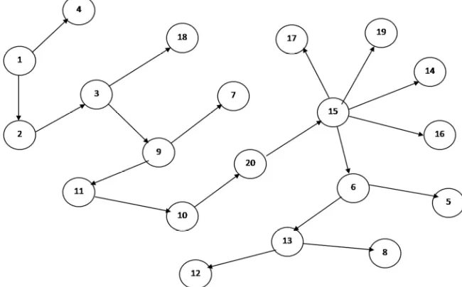
Figure 1 shows a typical example of CMST1 constructed from point set (from Dissimilarity matrix), in which inconsistent edges are removed to create subtree (clusters/regions).our algorithm finds the center of each clusters, which will be useful in many applications.
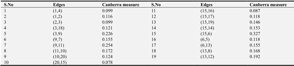
Table 3. Canberra distance based minimal spanning tree edges.
S.No Edges Canberra measure S.No Edges Canberra measure
1 (1,4) 0.099 11 (15,16) 0.087
2 (1,2) 0.116 12 (15,17) 0.118
3 (2,3) 0.099 13 (15,19) 0.146
4 (3,18) 0.121 14 (15,14) 0.153
5 (3,9) 0.226 15 (15,6) 0.327
6 (9,7) 0.155 16 (6,5) 0.118
7 (9,11) 0.254 17 (6,13) 0.155
8 (11,10) 0.172 18 (13,8) 0.168
9 (10,20) 0.124 19 (13,12) 0.192
10 (20,15) 0.078
Generally in most of the clustering algorithm data points can be represented as dissimilarity matrix representation. It contains the distance values between the data points represented as lower or upper triangular matrix. Our Canberra distance based minimal spanning tree algorithm constructs CMST1 from the dissimilarity matrix is shown figure 1. First to identify the longest edge in the CMST1 to generate subtree (clusters). Table 3, the longest edge weight 0.327 connecting the data points 15 and 6 is find to be inconsistent one. By removing the inconsistent edge from the CMST1, data points in the CMST1 partitioned into two subtrees or clusters T1andT2 namely.
{
}
1 1, 2, 3, 4, 7,9,10,11,14,15,16,17,18,19, 20
T = and
{
}
2 5, 6,8,12,13
T = . Secondly to find the center of T1 and
2
T using average of points, these centers is connected and again another minimal spanning tree CMST2 is constructed. The minimum edge of CMST2 is Emin =0.359and the maximum edge of CMST2 is Emax =0.359then to compute cluster separation value is 1. If the CS is greater than 0.8 then we conclude the subtrees or clusters created are well separated. Next to identify another longest edge weight from Table 3is 0.254 connecting the data points 9 and 11 is finding to be inconsistent one. By removing the inconsistent edge from the CMST1, data points partitioned into three sub trees or clustersT1,T2 and T3namely.
{
}
1 1, 2,3, 4, 7,9,18
T = , T2 =
{
10,11,14,15,16,17,19, 20}
and T3 =
{
5, 6,8,12,13}
. To compute the center of T1,T2and3
T using average of points, these centers is connected and again another minimal spanning tree CMST2 is constructed.
Table 4. Dissimilarity matrix.
Cluster-I Cluster-II Cluster-III Cluster-I 0.000 0.475 0.404 Cluster-II 0.000 0.465
Cluster-III 0.000
Table 5. Canberra distance based CMST2 edges.
S.No Edges Canberra measure
1 (1,3) 0.404
2 (3,2) 0.465
The minimum edge of CMST2 is Emin =0.404and the maximum edge of WMST2 is Emax =0.465then to compute
cluster separation value is 0.8688. If the CS is greater than 0.8 then we conclude the subtrees or clusters created are valid. Continuing this process, next to identify another longest edge weight from Table 3 is 0.226 connecting the data points 3 and 9 is finding to be inconsistent one. By removing the inconsistent edge from the CMST1, data points partitioned into three sub trees or clustersT1,T2,T3and T4namely.
{
}
1 1, 2, 3, 4,18
T = , T2 =
{
10,11,14,15,16,17,19, 20}
,{
}
3 5, 6,8,12,13
T = and T4 =
{ }
7, 9 . To compute the center of T1,T2,T3 and T4using average of points, these centers is connected and again another minimal spanning tree CMST2 is constructed.Table 6. Dissimilarity matrix.
Cluster-I Cluster-II Cluster-III Cluster-IV Cluster-I 0.000 0.533 0.494 0.265 Cluster-II 0.000 0.462 0.358 Cluster-III 0.000 0.271
Cluster-IV 0.000
Table 7. Canberra distance based CMST2 edges.
S.No Edges Canberra measure
1 (1,4) 0.265
2 (4,3) 0.271
3 (4,2) 0.358
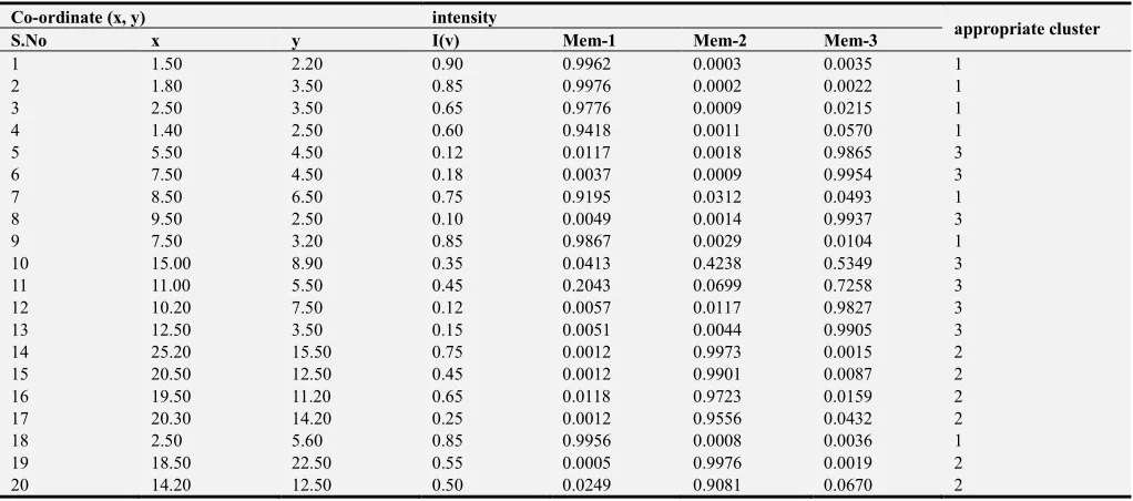
proposed KIFCM is much faster than the standard FCM and the method is converged fast to terminate condition with less run time. To test the effectiveness of KIFCM, the weighted minimal spanning tree based IFCM is used as center. This is done to find out the fuzzy membership and appropriate number of clusters. Thus, we have concluded the final optimal clusters formed as 3. This algorithm has also reduced
the number of iterations. Best result is achieved by this measure fuzzy partition coefficient Vpc maximum and
validation function Vp minimum (Table 10). The KIFCM
clustering algorithm has the following membership value intimacy (Table 8).
Table 8. Final membership of three clusters of intuitionistic FCM method and object allocation.
Co-ordinate (x, y) intensity
appropriate cluster
S.No x y I(v) Mem-1 Mem-2 Mem-3
1 1.50 2.20 0.90 0.9962 0.0003 0.0035 1 2 1.80 3.50 0.85 0.9976 0.0002 0.0022 1 3 2.50 3.50 0.65 0.9776 0.0009 0.0215 1 4 1.40 2.50 0.60 0.9418 0.0011 0.0570 1 5 5.50 4.50 0.12 0.0117 0.0018 0.9865 3 6 7.50 4.50 0.18 0.0037 0.0009 0.9954 3 7 8.50 6.50 0.75 0.9195 0.0312 0.0493 1 8 9.50 2.50 0.10 0.0049 0.0014 0.9937 3 9 7.50 3.20 0.85 0.9867 0.0029 0.0104 1 10 15.00 8.90 0.35 0.0413 0.4238 0.5349 3 11 11.00 5.50 0.45 0.2043 0.0699 0.7258 3 12 10.20 7.50 0.12 0.0057 0.0117 0.9827 3 13 12.50 3.50 0.15 0.0051 0.0044 0.9905 3 14 25.20 15.50 0.75 0.0012 0.9973 0.0015 2 15 20.50 12.50 0.45 0.0012 0.9901 0.0087 2 16 19.50 11.20 0.65 0.0118 0.9723 0.0159 2 17 20.30 14.20 0.25 0.0012 0.9556 0.0432 2 18 2.50 5.60 0.85 0.9956 0.0008 0.0036 1 19 18.50 22.50 0.55 0.0005 0.9976 0.0019 2 20 14.20 12.50 0.50 0.0249 0.9081 0.0670 2
Table 9. Comparison of iteration count.
No. of iterations No. of clusters
Standard FCM 14 3
IKFCM 5 3
MST based Intuitionistic FCM 2 3
Table 10. Cluster validity function.
Vpc Vp
Standard FCM 0.8997 0.1354
IKFCM 0.9088 0.1452
MST based Intuitionistic FCM 0.9124 0.1551
6.1. Statistical Evaluation of Diagnostic Performance of Mammography for Breast Cancer
Our study of random sample in terms of reported breast cancer associated symptoms and patient’s age group reveals that 10% of the patients had dense calcification, 10% had watery discharge from breast, 40% were complaining of lump, 30% had pain in breast tissues, 5% cases were having both lump and pain. While 5% were suffering from pain as well as discharge from breast tissues given in table 1. Patient’s data is categorized into two age groups; 25% cases belong to age group of 30-40 years while majority (75%) belongs to age group of 41-50 years. Mammography details revealed 33% were having benign tumor while malignancies were reported in 50% cases and 17% cases were diagnosed as normal shown in Table 11.
To evaluate the performance of diagnostic procedure for primary screening of breast cancer, initially specificity and sensitivity was calculated. Randomly select the sample dataset out of 60 patients subjected to mammography for detection of lump in mammary tissues, diagnosis reports analysis revealed 32 cases as TP, as disease was present in them while 04 false negative cases were observed in which diseases was present but symptoms or clinical presentation could not be evaluated through mammography. Likewise, 1 false positive case were reported through mammography and 23 true negative cases were also identified in which no indication of disease was observed. All the cases in terms of true positive (TP), true negative (TN), false positive (FP) and false negative (FN) are properly summarized in Table 12.
6.2. Sensitivity Percentage Result
True positive rate that defines the sensitivity of mammography in accurate detection of breast cancer in currently reported data was 88.89% shown in Table 13. In 60 cases, only four diseased cases were identified as false negative in mammogram evaluation. While it exactly reports majority of diseased cases as true positive. High sensitivity percentage corresponds to accurate detection of breast cancer patients of particular regions.
6.3. Specificity Percentage Result
True negative rate that defines the specificity of mammography in identification of non-diseases cases in our study sample was 95.83% shown in Table 13. In our study sample of 60 patients, 23 non-diseased cases were identified accurately as true negative through mammography. High specificity percentage corresponds to accurate identification of actual negative cases, this value also
state that mammography diagnosis is particularly dedicated to detection of breast lumps in patients.
6.4. Positive Likelihood Ratio and Negative Likelihood Ratio of Diagnostic Mammography
Positive likelihood ratio tells the outcome of a true positive result if lump is present and the probability of a true negative result if lump is absent. For our study sample dataset, value of positive likelihood ratio is 21.32% shown in Table 13. Its value corresponds to how well our diagnostic system can differentiate between true positive and false positive results. While negative likelihood ratio of probability of false negative test result in diseased case and the probability of a negative test result given that the lump in breast is absent. Negative likelihood ratio calculated for our study sample is 0.12% given in Table 13, which clearly demonstrate that system is well versed to identify true negative cases and give least prediction of false negative results.
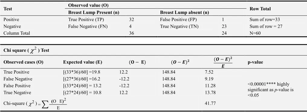
6.5. Pearson Chi-square (χχχχ2) Test Results
To evaluate the diagnostic accuracy of mammographic detection of breast cancer, Pearson Chi-square (χ2) test was performed to calculate predictive probability. Highly significant p-value (< 0.00001) indicates that for mammography based initial screening is a reliably diagnosed breast cancer in our study sample (Table 14). A highly significant correlation between mammography performance and clinical symptoms of breast cancer was observed in our study sample.
Table 11. Percentage distribution of study sample (n=60) based on age of disease presentation (years), breast cancer associated symptoms and nature of tumor.
Patient’s Factors %age
Age at diseases presentation (years)
30-40 25% (15)
41-50 75% (45)
Breast Cancer Associated Symptoms
Watery Discharge 10% (6) Calcification 10% (6)
Lump 40% (24)
Pain 30% (18)
Lump & Pain 5% (3) Pain and watery Discharge 5% (3) Nature of Tumor
Benign 33% (20) Malignant 50% (30) Normal 17% (10)
Table 12. Summary of total no of cases diagnosed through mammography as true positive (TP), false positive (FP), false negative (FN) and true negative (TN) in selected study sample.
Test Breast Lump Present (n) Breast LumpAbsent (no) Total
Positive True Positive (TP) 32 False Positive(FP) 1 TP +FP= 33 Negative False Negative (FN) 4 True Negative (TN) 23 FN + TN= 27
Table 13. Statistical analysis of Sensitivity, Specificity, Positive and Negative Likelihood ratio at95% CI to evaluate diagnostic accuracy of mammography for breast cancer detection.
S.No. Statistic Evaluation Formula Value
1 Sensitivity TP 100
TP+FN× 88.89%
2 Specificity TN 100
TN+FP× 95.83 %
3 Positive Likelihood Ratio
(
)
1Sensitivity Specificity
− 21.32
4 Negative Likelihood Ratio
(
1 Sensitivity)
Specificty
−
0.12
Table 14. Chi square test analysis for evaluation of diagnostic accuracy of mammography for breast cancer detection.
Test Observed value (O) Row Total
Breast Lump Present (n) Breast Lump absent (n)
Positive True Positive (TP) 32 False Positive (FP) 1 Sum of row=33 Negative False Negative (FN) 4 True Negative (TN) 23 Sum of row = 27
Column Total 36 24 N=60
Chi square (χ2) Test
Observed cases (O) Expected value (E) ( − ) ( − ) ( − ) p-value
True Positive [(33*36)/60] =19.8 12.2 148.84 7.52
<0.00001**** highly significant as p-value is <0.05
False Negative [(27*36)/60] =16.2 -12.2 148.84 9.19 False Positive [(33*24)/60] = 13.2 -12.2 148.84 11.28 True Negative [(27*24)/60] = 10.8 12.2 148.84 13.78
Chi-square (χ2)
∑
E E O =2
)
( 41.77
Formula of Expected value (E) [sum of row * sum of column/(n)].
7. Conclusion
Breast cancer is one of the major causes of death among women. Early diagnoses through regular screening and timely treatments have been demonstrated as the best prevention method for cancer. In this article, is introduced new alternative approach for breast cancer disease diagnosis and classifying benign and malignant breast cancer using MST initialization based Intuitionistic fuzzy c-means clustering algorithm for clear to identify of abnormalities for mammography images. We summarized the mammography results and evaluated the accuracy of mammography, 88.89% sensitivity, 95.83% specificity, 21.32 positive likelihood ratio, 0.12 negative likelihood ratios were calculated. It would be helpful to health professionals for making timely decisions for disease management in breast cancer patients. Also for future research, this method can be extended to apply real mammography images using Matlab, R-language and SPSS software.
Acknowledgements
We would like to thank the reviewers for their constructive comments. We thank to Dr. R. David chandrakumar, Professor, Department of Mathematics, Vickram College of Engineering, Madurai and Ms. K. Kavitha, Project Director,
District Rural Development Agency, Collectorate, Dindigul, for his encouragement and support given.
References
[1] Mayr FB, Yende S, Angus DC, Epidemiology of severe sepsis, Virulence, vol.5(1), pp.4-11(2014).
[2] Torre LA, Bray F, Siegel RL, Ferlay J, Lortet-Tieulent J, Jemal A, Global cancer statistics, CA: a cancer journal for clinicians, vol.65(2), pp.87-108 (2015).
[3] George J. Miao, Kathleen H. Miao, Julia H. Miao, “Neural pattern Recognition Model for Breast Cancer Diagnosis” Journal of selected areas in Bioinformatics, August edition, pp.1-8 (2012).
[4] S. Saheb Basha, Satya Prasad, “Automatic detection of breast cancer mass in mammograms using morphological operators and fuzzy c-means clustering” Journal of theoretical and applied information technology, pp. 704-709.
[5] Carlos Andres Pena-Reyes, Moshe Sipper, “A fuzzy-genetic approach to breast cancer diagnosis” Artificial Intelligence in Medicine, vol.17, pp. 131-155 (1999).
[7] Asif HM, Sultana S, Akhtar N, Rehman JU, Rehman RU, Prevalence, risk factors and disease knowledge of breast cancer in Pakistan, Asian Pac J Cancer Prev, vol.15(11), pp.4411-6 (2014).
[8] Steven D, Fitch M, Dhaliwal H, Kirk-Gardner R, Sevean P, Jamieson J, et al., editors. Knowledge, attitudes, beliefs, and practices regarding breast and cervical cancer screening in selected ethnocultural groups in Northwestern Ontario. Oncology nursing forum (2004).
[9] Coughlin SS, Thompson TD, Hall HI, Logan P, Uhler RJ. Breast and cervical carcinoma screening practices among women in rural and nonrural areas of the United States, 1998– 1999. Cancer, vol.94(11), pp.2801-12 (2002).
[10] Atanassov K. T, Intuitionistic fuzzy set past, present and future,
www.eusflat.org/publicaions/proceedings/.2003/./4Atanassov. pdf.
[11] Zhang H. M, Chen Z. S. Q, On clustering approach to intuitionistic fuzzy sets, control and decision. vol.22, pp.882-888 (2007).
[12] Chaira T, A novel intuitionistic fuzzyc-means clustering algorithm and its application to medical images, Applied soft computting, vol.11, pp.1711-1717 (2011).
[13] Prabhjot kaur, Soni A. K et, Novel Intuitionistic fuzzy c-means clustering for Linearly and nonlinearly separable data, Wseas transactions on computers, vol. 11(3), pp. 65-75 (2012).
[14] Dhirendra kumar, Hanuman verma, et, A modified intuitionistic fuzzy c-means clustering approach to segment human brain MRI image, Multimedia tools and applications, pp. 1-24 (2018).
[15] Damodar Reddy, Devender Mishra, et, MST-based cluster initialization for k-means, Berlin Springer-verlag, pp.329-338 (2010).
[16] Lan Huang, Shixian du, Yu Zhang et, K-means initial clustering center optimal algorithm based on kruskal, Journal of information & computational science, vol.9(9), pp.2387-239 (2012).
[17] Edward W. Packel, Functional Analysis, Intext Educational Publishers, NewYork (1974).
[18] Xie X. L and Beni G, A validity measure for fuzzy clustering. IEEE Trans. Pattern Anal. Mach. Intell., Vol. 3(8), pp-841-847(1991).
[19] Bezdek J. C., Hall L. O., Clarke L. P, Review of MR image segmentation techniques using pattern recognition, medical physics 20(4), pp. 1033-1048 (1993).
Biography
Nithya was born in 1992. She is a Research Scholar of Mathematics, Mother Teresa Womens University, Kodaikanal, Tamilnadu, India. His current research interests include digital topology, data mining and image processing.