PERFORMANCE ANALYSIS OF DIVIDE AND
CONQUER SORTING ALGORITHMS
Mrs. Sushma Nallamalli
1, Mrs. M. M. Vamsi Priya
21, 2
Associate Professor, CSE Dept, DMSSVH College of Engineering, Machilipatnam A.P, (India)
,
ABSTRACT
An algorithm is specification of a finite sequence of instructions to be carried out in order to solve a given problem. Sorting is considered as a fundamental operation in computer science as it is used as an intermediate step to manage datain many operations. Sorting refers to the process of arranging list of elements in a particular order. The elements are arranged in increasing or decreasing order of their key values. This research paper presents three different types of sorting algorithms using Divide and Conquer strategy like Merge sort, Quick sort, Shell sort and also gives their performance analysis with respect to time complexity along with the applications. These algorithms are important and have been an area of focus for a long time but still the question remains the same of “when to use which algorithm?” which is the main reason to perform this research. Each algorithm solves the sorting problem using the divide and conquer paradigm but in a different way. This research provides a detailed study of how all these algorithms work and then compares them on the basis of various parameters apart from time complexity with the help of their applications to reach our conclusion.
Keywords— Algorithm, Divide And Conquer, Merge Sort, Quick Sort, Shell Sort
I. INTRODUCTION
Sorting is an operation that segregates items into groups according to specified criterion. In data domain, sorting refers to the operation of arranging numerical data in increasing or decreasing order or non numerical data in alphabetical order. The usefulness and significance of sorting is depicted from the day to day application of sorting in real-life objects. For instance, objects are sorted in Telephone directories, income tax files, tables of contents, libraries, dictionaries. Sorting is a classic subject in computer science. There are three reasons [3] for studying sorting algorithms. First, sorting algorithms illustrate many creative approaches to problem solving and these approaches can be applied to solve other problems. Second, sorting algorithms are good for practicing fundamental programming techniques using selection statements, loops, methods, and arrays. Third, sorting algorithms are excellent examples to demonstrate algorithm performance. The performance analysis and design of useful sorting algorithms has remained one of the most important research areas in the field. Some algorithms are more efficient than others, in that less time or memory is required to execute them. The analysis [1] of algorithms studies time and memory requirements of algorithms and the way those requirements depend on the number of items being processed. The efficiency of a sorting algorithm depends on how fast and accurately it sorts a list and also how much space it requires in the memory.
The methods of sorting [1] can be divided into two categories:
An internal sort requires that the collection of data fit entirely in the computer‟s main memory.
The complexity of a sorting algorithm [8] measures the running time of function in which „n‟ number of items to be sorted. The choice of which sorting method is suitable for a problem depends on various efficiency considerations for different problem. Four most important of these considerations are: 1.The length of time spent by programmer in coding a particular sorting program. 2. Amount of machine time necessary for running the program. 3. The amount of memory necessary for running program. 4. Stability-does the sort preserves the order of keys with equal values.
II. ANALYSIS OF ALGORITHMS
A. Merge Sort
Merge sort was invented by John von Neumann in 1945.It is an O(n log n) comparison based sorting algorithm using divide and conquer strategy. In Divide-And-Conquer paradigm the problem is divided into a number of similar sub-problems of smaller size, Conquer the sub-problems by solving the sub-problems recursively, if the Sub-problem size is small enough, solve the problems in straightforward manner [9]. Combine the solutions of the sub-problems to obtain the solution for the original problem.
Conceptually, a merge sort works as follows
1. Divide the unsorted list into n sublists, each containing 1 element (a list of 1element is considered sorted). 2. Repeatedly merge sublists to produce new sublists until there is only 1 sublist remaining. This will be the sorted list.
In practical to sort an array A [p . . r]: Divide the n-element sequence to be sorted into two subsequences of n/2 elements each. Conquer by sorting the subsequences recursively using merge sort, when the size of the sequences is 1 there is nothing more to do combine by merging the two sorted subsequences.
2.1.1 Algorithm
MERGE-SORT (A, p, r) Begin
if p < r Check for base case
then q ← (p + r)/2 Divide MERGE-SORT (A, p, q) Conquer MERGE-SORT(A, q + 1, r) Conquer MERGE(A, p, q, r) Combine End
Initial call:MERGE-SORT(A, 1, n)
2.1.2 An Example
P q r
Divide:q=4
1 2 3 4 5 6 7 8
2.1.3 Conquer and Merge
T
2.1.4 Merge
Input: Array Aand indices p, q, rsuch that p ≤ q < r, Subarrays A [p . . q] and A[q + 1 . . r] are sorted
Output: One single sorted subarray A [p . . r].
Idea for merging: In Two piles of sorted cards, Choose the smaller of the two top cards, Remove it and place it in the output pile, Repeat the process until one pile is empty. Take the remaining input pile and place it face-down onto the output pile
1 2 3 4 5 6 7 8
6
3
2
1
7
5
4
2
p
q
r
1
5
22
34
47
1
6
3
72
86
51 2 3 4 5 6 7 8
7
6
5
4
3
2
2
1
1 2 3 4
7
5
4
2
5 6 7 8
6
3
2
1
1 2
5
2
3 4
7
4
5 6
3
1
7 8
6
2
1 2 3 4
7
4
2
5
5 6 7 8
6
2
3
1
1 2
2
5
3 4
7
4
5 6
3
1
7 8
6
2
15
22
34
47
1
Alg.: MERGE(A, p, q, r) 1. Compute n1 and n2
2. Copy the first n1 elements into L[1 . . n1 + 1] and the next n2 elements into R[1 . . n2 + 1]
3. L[n1 + 1] ← ; R[n2 + 1] ← 4. i ← 1; j ← 1
5. for k ← p to r 6. do if L[ i ] ≤ R[ j ]
7. then A[k] ← L[ i ]
8. i ←i + 1 9. else A[k] ← R[ j ]
10. j ← j + 1
2.1.5 Analysis
Analyzing Divide-and Conquer Algorithms [1]:The recurrence is based on the three steps of the paradigm:T(n) – running time on a problem of size n.Divide the problem into a subproblems, each of size n/b: takes
D(n).Conquer (solve) the subproblems aT(n/b) .Combine the solutions C(n)
T(n) = (1) if n ≤ c aT (n/b) + D(n) + C(n) otherwise MERGE-SORT Running Time:
Divide: Compute qas the average of pand r:D(n) = (1)
Conquer: Recursively solve 2 subproblems, each of size n/2 2T (n/2)
Combine: MERGE on an n-element subarray takes (n) time C(n) = (n)
The recurrence relation for the merge sort is as follows:
T(n) = (1) if n =1 2T(n/2) + c(n) if n > 1 Solve the Recurrence
p q
7
5
4
2
6
3
2
1
r q + 1
L
R
1 2 3 4 5 6 7 8
6
3
2
1
7
5
4
2
p
q
r
T(n) = c if n = 1 2T(n/2) + cn if n > 1
Use Master‟s Theorem [3]: Compare n with f(n) = cn then T(n) = Θ(n log n)
In short to analyze the time complexity of Merge Sort function, we need to consider the two distinct processes that makeup its implementation. First, the list is split into halves. We divide a list in half logn times where n is the length of the list. The second process is the merge. Each item in the list will eventually be processed and placed on the sorted list. So the merge operation which results in a list of size n requires n
operations. The result of this analysis is that logn splits, each of which costs n for a total of n (log n) operations. The best, average and the worst case time complexities are O (n logn) [8]. The Double Memory Merge Sort runs O (N log N) for all cases, because of its Divide and Conquer approach [4]. There are other variants of Merge Sorts including k-way merge sorting, but the common variant is the Double Memory Merge Sort. Though the running time is O(N log N) and runs much faster than insertion sort and bubble sort, merge sort‟s large memory demands makes it not very practical for main memory sorting.
2.1.6 Advantages and Disadvantages
2.1.6.1 Advantages
Time Complexity is O (nlogn).
Running time is insensitive of the input.
It can be used for both internal and external sorting
2.1.6.2 Disadvantages
At least twice the memory requirements of the other sorts because it is recursive.
Space complexity is very high as it requires extra space N.
2.1.7 Applications
To sort a huge randomly-ordered file of small records like process transaction record for a phone company, the merge sort is the best than any other sorting technique as the selection sort always takes quadratic time, bubble sort and insertion sort also takes quadratic time for randomly-ordered keys.
B. Quick Sort
Quick sort is developed by C. A. R. Hoare (1962). Quicksort is a divide-and-conquer sorting algorithm in which division is dynamically [1] carried out (as opposed to static division in Merge sort).
The three steps of Quicksort are as follows:
Divide: Rearrange the elements and split the array into two subarrays and an element in between such that each element in the left subarray is less than or equal to the middle element and each element in the right subarray is greater than the middle element.
Conquer: Recursively sort the two subarrays.
Combine: None.
2.2 Algorithm
Quicksort(A,n) 1: Quicksort‟(A,1,n) Quicksort‟ (A, p, r) 1: if p>=r then return 2: q=Partition(A,p,r) 3: Quicksort‟(A,p,q-1) 4: Quicksort‟(A,q+1,r) The subroutine Partition:
Given a subarray A[p..r] such that p<=r-1,this subroutine rearranges the input subarray into two subarrays, A[p…q-1]and A[q+1…r], so that each element in A[p..q -1]is less than or equal to A[q] and each element in A[q+1…r] is greater than or equal to A[q].Then the subroutine outputs the value of q.
Use the initial value of A[r] as the “pivot” in the sense that the keys are compared against it. Scan the keys A[p..r-1] from left to right and flush to the left all the keys that are greater than or equal to the pivot.
The Algorithm Partition(A,p,r) 1: x=A[r] 2: i=p-1
3: for j=p to r-1do 4: if A[j]<=x then {
5: i= i+1
6: Exchange A[i] andA[j] }
7: Exchange A[i+1] and A[r] 8: return i+1
2.2.1 Analysis
merge-sort, since there are no comparisons involved in the conquer phase. The best-case input is a sequence that has all subsequences produced by splitting with the same mean as their median, since this produces the fewest number of levels. The worst-case input for splitting on the mean is a geometric series sorted in opposite order to the desired sorting order. The time complexity ranges between n log(n) and n2 depending on the key distribution and the pivot choices.
Best Case = O(n log n) Average Case=O (n log n) Worst Case= O (n2)
2.2.2 Advantages and Disadvantages
2.2.2.1 Advantages
One of the fastest algorithms on average.
Does not need additional memory (the sorting takes place in the array-In-place processing).
The list is being traversed sequentially, which produces very good locality of reference and cache behavior
for arrays.
2.2.2.2 Disadvantages
Space used in the average case for implementing recursive function calls is O (log n) and hence proves to
be a bit space costly, especially when it comes to large data sets.
The worst-case complexity is O(n2) .
2.2.2.3 Applications
Commercial applications use Quicksort as it runs fast, no additional memory, this compensates for the rare occasions when it runs with (O(n2).Never use in applications which require guaranteed response time. Life critical (medical monitoring, life support in aircraft and space craft), Mission-critical(monitoring and control in industrial and research plants handling dangerous materials, control for aircraft ,defense, etc) unless you assume the worst-case response time.
C. Shell Sort
The principle of Shell sort is to rearrange the file so that looking at every hth element yields a sorted file. We call such a file h-sorted. If the file is then k-sorted for some other integer k, then the file remains h-sorted. For instance, if a list was 5-sorted and then 3-sorted, the list is now not only 3-sorted, but both 5 and 3 sorted. The algorithm draws upon a sequence of positive integers known as the increment sequence. Any sequence will do, as long as it ends with 1, but some sequences perform better than others. The algorithm begins by performing a gap insertion sort, with the gap being the first number in the increment sequence. It continues to perform a gap insertion sort for each number in the sequence, until it finishes with a gap of 1. When the increment reaches 1, the gap insertion sort is simply an ordinary insertion sort, guaranteeing that the final list is sorted. Beginning with large increments allows elements in the file to move quickly towards their final positions, and makes it easier to subsequently sort for smaller increments. Although sorting algorithms exist that are more efficient, Shell sort remains a good choice for moderately large files because it has good running time and is easy to code.
Shell Sort represents a "divide-and-conquer"[6] approach to the problem.
That is, we break a large problem into smaller parts (which are presumably more manageable), handle each part, and then somehow recombine the separate results to achieve a final solution. In Shell Sort, the recombination is achieved by decreasing the step size to 1, and physically keeping the sublists within the original list structure.
2.3 Algorithm
Input: An array a of length n with array elements numbered 0 to n − 1 inc ← round(n/2)
while inc > 0 do:
for i = inc .. n − 1 do: temp ← a[i] j ← i
while j ≥ inc and a[j − inc] > temp do: a[j] ← a[j − inc]
j ← j − inc a[j] ← temp inc ← round(inc / 2.2)
The increment sequence is a geometric sequence in which every term is roughly 2.2 times smaller than the previous one.
An Example
Sort: 18 32 12 5 38 33 16 2
8 numbers to be sorted, shell‟s increment will be floor (n/2)
*floor(8/2) floor(4)=4
Increment 4: 1 2 3 4 (visualize coloring) 18 32 12 5 38 33 16 2
Step 1) Only look at 18 and 38and sort in order .
18and 38 stays at its current position because they are in order. Step 2) Only look at 32and 33 and sort in order .
12 and 16 stays at its current position because they are in order. Step 4) Only look at 5and 2and sort in order .
2 and 5 need to be switched to be in order. Resulting numbers after increment 4 pass:
18 32 12 2 38 33 16 5 * floor(4/2) floor(2) = 2
Increment 2:1 2
18 32 12 2 38 33 16 5
Step 1) Look at 18, 12, 38, 16 and sort them in their appropriate location:
12 38 16 2 18 33 38 5
Step 2) Look at 32, 2, 33, 5 and sort them in their appropriate location:
12 2 16 5 18 32 38 33
Resulting numbers after increment 2 pass:
12 2 16 5 18 32 38 33
* floor(2/2) floor(1) = 1
Increment 1: 1
12 2 16 5 18 32 38 33
2 5 12 16 18 32 33 38
The last increment or phase of Shellsort is basically an Insertion Sort algorithm.
2.3.1 Analysis
Efficiency of shell sort depends on the values of increment h. In Shell's original sequence h is N/2 , N/4,..1 (repeatedly divide by 2),Hibbard's increments are 1, 3, 7,., 2k - 1 ,Knuth's increments[2] are 1, 4,13,, ( 3k - 1)/ 2.Start with 1,then multiply by 3 and add 1.This takes less than O(n3/2) comparisons and Sedgewick's increments:1, 5, 19, 41, 109, .... 9 ·4k - 9 ·2k + 1 or 4k - 3 ·2k + 1.Shellsort's worst-case performance using Hibbard's increments is Θ(n3/2). The average performance is thought to be about O(n 5/4) .The exact complexity of this algorithm is still being debated .This is better for mid-sized data nearly as well if not better than the faster (n log n) sorts. The Shell‟s original sequence is treated as a Bad sequence because elements in odd positions are not compared to elements in even positions until the final pass. Shellsort does less than O(N(log N)2) comparisons for the increments 1 2 3 4 6 9 8 12 18 27. . .Analysis is complicated. Increments should be relatively prime (i.e., share no common factors). This guarantees that successive passes intermingle sublists so that the entire list is almost sorted before the final pass. With well-chosen increments, efficiency can approach O(N(logN)(logN)) or N logN-squared. Its general analysis is an open research problem. Performance depends on sequence of gap values like for sequence 2k, performance is O(n2) Hibbard‟s sequence (2k-1), performance is O(n3/2) We start with n/2 and repeatedly divide by 2.2 Empirical results show this is O(n5/4) or O(n7/6).No theoretical basis (proof) that this holds.
2.3.2 Advantages and Disadvantages
2.3.2.1 Advantages
Only efficient for medium size lists.
2.3.2.2 Disadvantages
It is a complex algorithm and its not nearly as efficient as the merge, heap, and quick sorts.
Itis significantly slower than the merge, heap, and quick sorts.
2.3.3 Applications
Shell sort is now rarely used in serious applications. It performs more operations and has higher cache miss ratio than quicksort. However, since it can be implemented using little code and does not use the call stack, some implementations of the qsort function in the C standard library targeted at embedded systems use it instead of quicksort. Shellsort is, for example, used in the uClibc library. For similar reasons, an implementation of Shellsort is present in the Linux kernel.Shellsort can also serve as a sub-algorithm of introspective sort, to sort short subarrays and to prevent a pathological slowdown when the recursion depth exceeds a given limit. This principle is employed, for instance, in the bzip2 compressor.
III. COMPARITIVE STUDY OF ALGORITHMS
Table I-Complexity Comparison
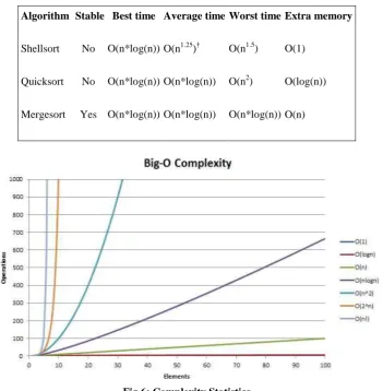
Algorithm Stable Best time Average time Worst time Extra memory
Shellsort No O(n*log(n)) O(n1.25)† O(n1.5) O(1)
Quicksort No O(n*log(n)) O(n*log(n)) O(n2) O(log(n))
Mergesort Yes O(n*log(n)) O(n*log(n)) O(n*log(n)) O(n)
Fig 6: Complexity Statistics
Sorting analysis summary
IV. C
ONCLUSIONIn this paper, we got into sorting problem and investigated different solutions. We talked about the most popular sorting algorithms using the divide and conquer strategy. They are: Merge sort, Quick sort and Shell sort. Algorithms were represented with perfect descriptions and examples. Also, it was tried to indicate the computational complexity of them in the worst, middle and best cases along with the applications and pros and cons. At the end, we can analyze that Merge sort can be used for huge randomly ordered files of small records but with a little bit of memory requirements. On an average Quick sort is the best unless you assume the worst-case response time. Shell sort is recently replacing some of the quick sort applications due to its little code and no recursion. Finally we can conclude that Good algorithms are better than supercomputers but great algorithms are better than good ones.
REFERENCES
[1] Wikipedia. Address: http://www.wikipedia.com
[2] Donald Knuth. The Art of Computer Programming, Volume 3: Sorting and Searching, Second Edition. Addison- Wesley, 1998. ISBN 0-201-89685-0. Pages 106–110 of section 5.2.2: Sorting by Exchanging. [3] Weiss, Mark Allen (1997). Data Structures and Algorithm Analysis in C. Addison Wesley Longman. pp.
222–226.
[4] Computer Algorithms by Ellis Horowitz, Sartaj Sahni, Sanguthevar Rajasekaran, Galgotia publications,5 Ansari road, Daryaganj, New Delhi-110002
[5] C.A.R. Hoare, Quicksort, Computer Journal, Vol. 5, 1, 10-15 (1962) World Applied Programming, Vol (1), No (1), April 2011. 62-71 ISSN: 2222-2510 ©2011 WAP journal.
[6] Popular sorting algorithms C. Canaan * M. S. Garai M. DayaInformation institute Chiredzi, Zimbabwe [7] Source code examples based on "A Practical Introduction to Data Structures and Algorithm Analysis" by
Clifford A. Shaffer, Prentice Hall, 1998. Copyright 1998 by Clifford A. Shaffer.
[8] Pooja et al., International Journal of Advanced Research in Computer Science and Software Engineering 3(11), November - 2013, pp. 500-507