University of Pennsylvania
ScholarlyCommons
Publicly Accessible Penn Dissertations
2017
Efficient Baseline Utilization In Crossover Clinical
Trials Through Linear Combinations Of Baselines:
Parametric, Nonparametric, And Model Selection
Approaches
Thomas Jemielita
University of Pennsylvania, [email protected]
Follow this and additional works at:
https://repository.upenn.edu/edissertations
Part of the
Biostatistics Commons
This paper is posted at ScholarlyCommons.https://repository.upenn.edu/edissertations/2360
For more information, please [email protected].
Recommended Citation
Jemielita, Thomas, "Efficient Baseline Utilization In Crossover Clinical Trials Through Linear Combinations Of Baselines: Parametric, Nonparametric, And Model Selection Approaches" (2017).Publicly Accessible Penn Dissertations. 2360.
Efficient Baseline Utilization In Crossover Clinical Trials Through Linear
Combinations Of Baselines: Parametric, Nonparametric, And Model
Selection Approaches
Abstract
In a crossover clinical trial, including period-specific baselines as covariates in a regression model is known to
increase the precision of the estimated treatment effect. The potential efficiency gain depends, in part, on the
true model, the distribution and covariance matrix of the vector of baselines and outcomes, and the model
chosen for analysis. We examine improvements in power that can be achieved by incorporating optimal linear
combination of baselines (LCB). For a known distribution, the optimal LCB minimizes the conditional
variance corresponding to a treatment effect. The use of a single metric to capture the information in the
baseline measurements is appealing for crossover designs. Because of their efficiency, crossover designs tend
to have small sample sizes and thus the number of covariates in a model can significantly impact the degrees of
freedom in the analysis. We start by examining optimal LCB models under a normality assumption for
uniform and incomplete block designs. For uniform designs, such as the AB/BA design, estimation is entirely
through within-subject contrasts (and thus ordinary least squares [OLS]) and the optimal LCB minimizes the
conditional variance corresponding to the treatment effect. However, since the optimal LCB is a function of
the unknown covariance matrix, we propose an adaptive method that uses the LCB covariate corresponding
to the most plausible covariance structure guided by the data. For incomplete block designs, data are
commonly analyzed using a mixed effects model. Treatment effect estimates from this analysis are complex
functions of both within-subject and between-subject treatment contrasts. To improve efficiency, we propose
incorporating period-specific optimal LCBs which minimize the conditional variance of the period-specific
outcomes. A simpler fixed effects analysis of covariance involving only within-subject contrasts is also
described for small sample situations. In the latter, hypothesis tests based on the mixed effects analyses exhibit
inflated type I error rates even when using a Kenward and Rogers approach to adjust the degrees of freedom.
Lastly, we extend this work to the more general setting where the optimal LCB depends on the distribution of
the response vector. In practice, the distribution is unknown and the optimal LCB is estimated under some
loss function. To handle both normal and non-normal response data, OLS and a rank-based nonparametric
regression model (R-estimation), are considered. A data-driven approach is then proposed which adaptively
chooses the best fitting model among a set of models which work well under a range of conditions. Relative to
commonly used methods, such as change from baseline analyses without use of covariates, our methods using
functions of baselines as period-specific or period-invariant covariates consistently demonstrate improved
power across a number of crossover designs, covariance structures, and response distributions.
Degree Type
Dissertation
Degree Name
Doctor of Philosophy (PhD)
Graduate Group
First Advisor
Mary E. Putt
Second Advisor
Devan V. Mehrotra
Keywords
Baselines, Crossover trials, Longitudinal Analysis, Model Selection, Nonparametric regression, Robust
Estimation
Subject Categories
EFFICIENT BASELINE UTILIZATION IN CROSSOVER CLINICAL TRIALS THROUGH LINEAR COMBINATIONS OF BASELINES: PARAMETRIC, NONPARAMETRIC, AND MODEL
SELECTION APPROACHES
Thomas O. Jemielita
A DISSERTATION
in
Epidemiology and Biostatistics
Presented to the Faculties of the University of Pennsylvania
in
Partial Fulfillment of the Requirements for the
Degree of Doctor of Philosophy
2017
Supervisor of Dissertation Co-Supervisor of Dissertation
Mary E. Putt Devan V. Mehrotra, Adjunct Associate Professor of Biostatistics
Professor of Biostatistics Associate Vice President in Biostatistics, Merck & Co.
Graduate Group Chairperson
Nandita Mitra, Professor of Biostatistics
Dissertation Committee
Kathleen J. Propert, Professor of Biostatistics
Justine Shults, Professor of Biostatistics
Michelle Denburg, Assistant Professor of Pediatrics at the Children’s Hospital of Philadelphia
EFFICIENT BASELINE UTILIZATION IN CROSSOVER CLINICAL TRIALS THROUGH LINEAR
COMBINATIONS OF BASELINES: PARAMETRIC, NONPARAMETRIC, AND MODEL
SELECTION APPROACHES
c
COPYRIGHT
2017
Thomas O. Jemielita
This work is licensed under the
Creative Commons Attribution
NonCommercial-ShareAlike 3.0
License
To view a copy of this license, visit
ACKNOWLEDGEMENT
My experience at the University of Pennsylvania has been amazing. To start, I would like to thank
my two co-advisors Mary Putt and Devan Mehrotra. I really have learned a lot from Mary and Devan
and couldn’t imagine having better advisors. I appreciate the time, knowledge, and wisdom they
put into helping me develop a quality dissertation. Their continual guidance and expertise has truly
made the dissertation experience rewarding. I would also like to express my gratitude to the rest
of my committee members, Dr. Kathleen Propert, Dr. Justine Shults, Dr. Michelle Denburg, and
Dr. Inna Chervoneva, for their feedback and support throughout the dissertation process. Their
insights were essential for this dissertation research.
I also want to thank Dr. Jason Roy and Dr. Kathleen Propert for their support during my masters
thesis. I would like to again thank Dr. Michelle Denburg and Dr. Justine Shults for their guidance
on the renal training grant. I also would like to thank Dr. Richard Landis and Dr. Alisa Stephens
for their mentorship through my tenure on the MAPP research group. To the whole MAPP research
group, thank you for the valuable experience and fun memories. A special note of recognition goes
to all the Upenn biostats students who made my time at Upenn truly memorable, both at school and
outside of school.
Finally, I need to thank my incredible wife Brittany Oakes Jemielita, who I met at Upenn, for her love
and support throughout my PhD studies. I could always count on her for help and motivation and I
couldn’t have done this without her. I would also like to thank my parents, Kim Severson and Philip
Jemielita, for their never-ending support and advice. I would also like to thank the following friends
and family: Matthew Jemielita, Isaac Jemielita, Hector Jemielita, Ollie Jemielita, Sarah Morejohn,
ABSTRACT
EFFICIENTBASELINEUTILIZATIONINCROSSOVERCLINICALTRIALSTHROUGHLINEAR
COMBINATIONSOFBASELINES:PARAMETRIC,NONPARAMETRIC,ANDMODEL
SELECTIONAPPROACHES
ThomasO.Jemielita
MaryE.Putt
DevanV.Mehrotra
Inacrossoverclinicaltrial,includingperiod-specificbaselinesascovariatesinaregressionmodel
isknownto increasetheprecisionof theestimatedtreatmenteffect. Thepotential efficiencygain
depends,inpart,onthetruemodel,thedistributionandcovariancematrixofthevectorofbaselines
andoutcomes,andthemodelchosenforanalysis.Weexamineimprovementsinpowerthatcanbe
achievedbyincorporatingoptimallinearcombinationofbaselines(LCB).Foraknowndistribution,
theoptimalLCBminimizestheconditionalvariancecorrespondingtoatreatmenteffect.Theuseof
asinglemetrictocapturetheinformationinthebaselinemeasurementsisappealingforcrossover
designs. Becauseof theirefficiency,crossoverdesignstendtohavesmallsamplesizesandthus
thenumberofcovariatesina modelcan significantlyi mpactt hed egreeso ff reedomi nt he
anal-ysis. We startby examiningoptimal LCB models under anormality assumption for uniformand
incompleteblock designs. Foruniformdesigns, suchastheAB/BAdesign, estimationisentirely
throughwithin-subjectcontrasts(andthusordinaryleastsquares[OLS])andtheoptimalLCB
min-imizestheconditionalvariancecorrespondingtothetreatmenteffect. However,sincetheoptimal
LCBisafunctionoftheunknowncovariancematrix,weproposeanadaptivemethodthatusesthe
LCBcovariate correspondingto themost plausiblecovariancestructure guidedby thedata. For
incompleteblockdesigns,dataarecommonlyanalyzedusingamixedeffectsmodel.Treatment
ef-fectestimatesfromthisanalysisarecomplexfunctionsofbothwithin-subjectandbetween-subject
treatmentcontrasts. Toimproveefficiency,weproposeincorporatingperiod-specificoptimalLCBs
which minimizethe conditional variance of theperiod-specifico utcomes.A s implerfi xedeffects
analysis of covariance involving only within-subjectcontrasts is also described for small sample
I error rates even when using a Kenward and Rogers approach to adjust the degrees of freedom.
Lastly, we extend this work to the more general setting where the optimal LCB depends on the
distribution of the response vector. In practice, the distribution is unknown and the optimal LCB is
estimated under some loss function. To handle both normal and non-normal response data, OLS
and a rank-based nonparametric regression model (R-estimation), are considered. A data-driven
approach is then proposed which adaptively chooses the best fitting model among a set of
mod-els which work well under a range of conditions. Relative to commonly used methods, such as
change from baseline analyses without use of covariates, our methods using functions of baselines
as period-specific or period-invariant covariates consistently demonstrate improved power across
TABLE OF CONTENTS
ACKNOWLEDGEMENT . . . iii
ABSTRACT . . . iv
LIST OF TABLES . . . viii
LIST OF ILLUSTRATIONS . . . ix
CHAPTER 1 : INTRODUCTION . . . 1
CHAPTER 2 : UNIFORMDESIGNS . . . 3
2.1 Motivation and Literature Review . . . 3
2.2 Model and Notation . . . 5
2.3 Choosing the Optimal Linear Combination of Baselines (LCB) . . . 8
2.4 Estimation . . . 10
2.5 Application to Uniform Crossover Designs . . . 12
2.6 Application to Data Analysis . . . 17
2.7 Simulations . . . 19
2.8 Discussion . . . 25
CHAPTER 3 : INCOMPLETEBLOCKDESIGNS. . . 28
3.1 Motivation and Literature Review . . . 28
3.2 Setup and Notation . . . 30
3.3 Baseline Models . . . 32
3.4 Estimation . . . 41
3.5 Application to a Clinical Trial . . . 43
3.6 Simulations . . . 43
3.7 Discussion . . . 46
4.1 Motivation and Literature Review . . . 50
4.2 Models and Notation . . . 53
4.3 Estimation and Hypothesis Testing . . . 55
4.4 Selecting the LCB . . . 58
4.5 Model Selection and Inference: A Bootstrap Approach . . . 60
4.6 Application of Methods . . . 62
4.7 Simulations . . . 66
4.8 Real Data Analysis . . . 73
4.9 Discussion . . . 77
CHAPTER 5 : CONCLUSION . . . 80
APPENDICES . . . 82
LIST OF TABLES
TABLE 2.1 : Covariance Structure Assumptions: CS, DCS, EP, and AR(1) . . . 14
TABLE 2.2 : Uniform Design: Optimal LCB by Design and Covariance Structure . . . 16
TABLE 2.3 : Uniform Design Baseline Models: 2×2Real Data Example I (N=20) . . . . 18
TABLE 2.4 : Uniform Design Baseline Models: 3×3Real Data Example (N=24) . . . 19
TABLE 2.5 : 2×2Simulations: Under the Alternative Hypothesis, Power . . . 22
TABLE 2.6 : 3×3Simulations: Under the Alternative Hypothesis, Power . . . 23
TABLE 2.7 : 4×4Simulations: Under the Alternative Hypothesis, Power . . . 24
TABLE 3.1 : Baseline Utilization Methods: Incomplete Block Design . . . 39
TABLE 3.2 : Real Data Example: 3×2Crossover Design . . . 43
TABLE 3.3 : 3×2Simulations: Under the Null Hypothesis, Type I Error . . . 46
TABLE 3.4 : 3×2Simulations: Under the Alternative Hypothesis, Power . . . 47
TABLE 4.1 : Crossover Design Optimal Modeling Strategies . . . 60
TABLE 4.2 : Parametric and Nonparametric Crossover Models . . . 64
TABLE 4.3 : 2×2Simulations: Estimated LCBs . . . 68
TABLE 4.4 : Parametric and Nonparametric Comparisons: 2×2 Real Data Example I (N=20) . . . 75
TABLE 4.5 : Parametric and Nonparametric Comparisons: 2×2 Real Data Example II (N=24) . . . 76
TABLE 4.6 : Parametric and Nonparametric Comparisons:3×3Real Data Example (N=24) 77 TABLE A.1 : Notation . . . 82
TABLE B.1 : Treatment Effect Sizes: 2×2,3×3and4×4Design . . . 92
TABLE B.2 : 2×2Simulations: Under the Null Hypothesis, Type I Error . . . 94
TABLE B.3 : 3×3Simulations: Under the Null Hypothesis, Type I Error . . . 95
TABLE B.4 : 4×4Simulations: Under the Null Hypothesis, Type I Error . . . 96
TABLE D.1 : Parametric and Nonparametric Comparisons,2×2Simulations: Type I Error 109 TABLE D.2 : Parametric and Nonparametric Comparisons,2×2Simulations: Power . . . 110
LIST OF ILLUSTRATIONS
FIGURE 4.1 : 2x2 Simulations: Benchmark Comparisons . . . 69
FIGURE 4.2 : 2x2 Simulations: Min-P Comparisons . . . 70
FIGURE 4.3 : 3x3 Simulations: Benchmark Comparisons . . . 71
FIGURE 4.4 : 3x3 Simulations: Min-P Comparisons . . . 72
CHAPTER 1
I
NTRODUCTIONA crossover trial is a repeated measures design in which patients receive sequences of treatments
administered over some number of pre-specified periods. In contrast to a parallel group trial where
patients are randomized to specific treatment arms, crossover designs randomize subjects by
se-quence. One advantage of this design is that the estimate of a treatment effect is obtained wholly
or mostly through within-subject contrasts. Relative to a parallel group trial, this leads to large
efficiency gains and thus fewer enrolled subjects are required.
The crossover design is defined by the chosen sequences of treatments. A sequence depends on
the number of periods and the ordering of the considered treatments. For example, in the AB/BA or
2×2(2-treatment, 2-period) design, subjects are randomized to either sequence AB or sequence
BA. In sequence AB, subjects receive treatment A followed by treatment B. The order is reversed for
subjects in sequence BA. The primary disadvantage of a crossover design is the possibility that a
treatment effect can linger into the following period. This is called carryover and can complicate the
estimation of treatment effects (Jones and Kenward, 2003). A washout period is typically included
between periods to minimize the risk of carryover. In a pharmaceutical setting, pharmacokinetics
can be used to determine an appropriate length for the washout, such that any carrover is mitigated.
For the purposes of this dissertation, carryover is assumed to be null, or where the washout periods
are sufficient.
For a design with a continuous outcome of interest (e.g. blood pressure), the outcome is typically
measured prior to the period-specific treatment administration. These measurements are called
period-specific baselines, or just baselines. For the AB/BA design, each subject has two baseline
measurements and two treatment or outcome measurements. Often, the baseline and
post-treatment measurements are at least moderately correlated (Kenward and Roger, 2010; Mehrotra,
2014). Thus, including the baselines as covariates in a regression model has the potential to reduce
the standard error of a treatment estimate and increase the overall power to detect a treatment
effect. The overall goal of this research is to efficiently incorporate baselines into the analysis of a
There has been considerable work in baseline utilization in crossover designs, primarily for the
AB/BA design. Our work expands on this previous research and builds a general framework for
efficient baseline utilization for a variety of designs and regression models. Specifically, we
ex-amine improvements in power that can be achieved by incorporating optimal linear combinations
of baselines (LCB). For a known distribution, the optimal LCB minimizes the conditional variance
corresponding to a treatment effect. Further, given that crosover designs typically have small
sam-ple sizes, the number of covariates in a regression model can significantly impact the degrees of
freedom and consequently the efficiency of a hypothesis test. Thus, the optimal LCB preserves
the limited number of degrees of freedom while explicitly reducing the variance of a treatment
ef-fect estimate. Overall, this can greatly increase the efficiency of a hypothesis test. Compared to
standard baseline models such as the change from baseline model, our proposed LCB baseline
models yield substantial efficiency gains.
Chapters 2-3 respectively discuss efficient baseline utilization under a normality assumption for
uni-form and incomplete block designs. For the uniuni-form design, estimation of a treatment effect comes
entirely from within-subject contrasts and the optimal LCB minimizes the conditional variance
re-lated to the contrasts. For the incomplete block design, estimation of a treatment effect does not
necessarily need to come from only within-subject contrasts. Consequently, baseline utilization is
explored in the framework of both mixed models, where estimation is a weighted summation of
withsubject and between-subject information, and also models which only use withsubject
in-formation. Chapter 4 extends this work to a more general setting where the optimal LCB depends
on some known distribution. A framework is developed for efficient baseline utilization under a
general regression model. This naturally extends the research in Chapters 2-3 to non-normal
dis-tributions. For practical implementation, data-driven adaptive methods are proposed in all cases.
Lastly, Chapter 5 summarizes the overall findings and main points. A summary of most notations,
CHAPTER 2
U
NIFORMD
ESIGNS2.1. Motivation and Literature Review
The research in this Chapter appears in Statistics in Medicine (Jemielita, Putt, and Mehrotra, 2016).
One of the most commonly used crossover designs is the uniform design. A uniform design is both
uniform within sequence, each treatment appears the same number of times within each sequence,
and uniform within period, each treatment appears the same number of times within each period.
For example, the AB/BA design is considered uniform since each treatment appears once in each
sequence and once in each period. In general, designs that are both uniform within sequence
and uniform within period and thus uniform are efficient under commonly used models since all
estimation is through within-subject constrasts.
Over the years, a number of publications have considered incorporating baseline measurements
into the analysis of crossover designs. One of the recurring themes in this literature involves the
importance of the underlying covariance structure in determining how incorporating baselines into
the analysis can improve the precision of the treatment estimate. Hills and Armitage first noted
that the correlation between the baselines and outcomes was a driving factor in deciding whether
or not to use baselines (Armitage and Hills, 1982; Hills and Armitage, 1979). Kenward and Jones
explored different estimation techniques when incorporating baselines, including least squares and
generalized least squares (GLS) (Kenward and Jones, 1987). Building on earlier work, Kenward
and Roger established a clear theoretical framework to illustrate how the underlying covariance
structure of the baselines and outcomes influence bias and efficiency when the baselines are
in-corporated into the analysis using several different methods (Kenward and Roger, 2010). Metcalfe
explored using baselines as covariates in the AB/BA design through analysis of covariance
(AN-COVA) using the difference between the baselines at period 1 and period 2 as a covariate (Metcalfe,
2010). Metcalfe empirically showed that this covariate yielded improved efficiency across a
num-ber of covariance structures, relative to using change scores (post-treatment minus the baselines)
or using post-treatment measurements only. Chen, Meng and Zhang examined joint modeling of
(Chen, Meng, and Zhang, 2012). This work, through theoretical arguments and empirical
simu-lations, illustrated that including baselines in the analysis could improve the efficiency of a
treat-ment effect estimate. Most recently, Mehrotra in agreetreat-ment with previous authors, showed that the
potential efficiency gained by using baselines as covariates is highly influenced by the covariance
structure of the baselines and post-treatment outcomes (Mehrotra, 2014). Using theory and
simula-tions, Mehrotra examined ten different baseline utilization methods for the AB/BA crossover design
across a number of underlying baseline and outcome covariance structures and sample sizes. His
final recommendation was to use the difference between baselines at period 1 and period 2 as a
covariate in ANCOVA.
Our review of the literature thus suggests that the potential gains in efficiency that result from
incorporating baselines into an analysis demonstrate a strong model-dependence, both in terms
of the structure of the fixed effects model and the covariance structure. In the research reported
here we use the simplest possible model for the carryover, and assume that carryover is eliminated
by the washout. This is especially reasonable in a pharmaceutical setting, since pharmacokinetics
can be used to determine an appropriate length for the washout period. The current work builds on
previous findings by Mehrotra and Metcalfe (Mehrotra, 2014; Metcalfe, 2010). For the AB/BA under
a model with no carryover and a number of difference covariance structures, these authors showed
that using the using the difference in period-specific baselines as a covariate offered increased
precision for the estimate of the treatment effect.
The use of a single linear combination to capture the information in the baseline measurements
is appealing for crossover designs. Because of their efficiency, crossover studies often use small
sample sizes, and thus the number of covariates in the model can significantly impact the degrees
of freedom in the analysis. We begin by developing a theoretical framework to determine an optimal
linear combination of baselines for uniform designs, first under an unstructured covariance
assump-tion, and then using several different plausible assumptions for the covariance structure. Because
the covariance structure in a data analysis is unknown, we develop a data-based ’adaptive’ method
to choose the optimal covariate. We then apply this work to the AB/BA design and to the three
and four-period uniform designs, where the commonly used compound symmetry assumption is
increasingly unlikely to realistically represent the covariance structure of data obtained in practice.
base-lines can lead to significant efficiency gains.
The model and notation for a general uniform crossover design are defined in Section 2.2. In
Sec-tion 2.3, we describe the proposed method for choosing a baseline covariate. SecSec-tion 2.4 covers
estimation for the proposed method. Section 2.5 covers the application of the proposed methods
for2×2,3×3, and4×4crossover designs and explores various plausible covariance structures for
the post-treatment measurements and baselines. Additionally, we describe the optimal baseline
co-variates under each covariance structure and crossover design and illustrate how to implement our
approach using a data driven ’adaptive’ method. In Section 2.6, we evaluate our proposed methods
on real data sets. In section 2.7, our proposed methods are evaluated through simulations for2×2,
3×3, and4×4crossover designs. Lastly, in section 2.8, we summarize the overall findings.
2.2. Model and Notation
Assume a uniform crossover design. Let:
Xik= (XiAk, ..., XiZk)T
Yik= (YiAk, ..., YiZk)T (2.1)
be distinctZ-vectors of baseline and outcome measurements respectively, wherei= 1, .., sindexes
sequence,d=A, ..., Z indexes treatment, andj= 1, ..., pindexes the period. For this Chapter, we
focus on uniform crosssover designs where the number of periods equals the number of treatments
(p=Z). Lastly,k = 1, ..., ni indexes subjectkin sequencei, where subjects are assumed to be
independent of each other. Initially, we consider a ’sequence-invariant’ approach where we order
the outcomes and baselines within each sequence by treatment. Later, as well as in Chapters 3-4,
we generalize our approach to the case where each subject retains the vector of outcomes in the
order in which they are received. We then assume multivariate normality such that:
Xik Yik
∼N
E(Xik)
E(Yik)
,
ΣXX ΣXY ΣT
XY ΣY Y
!
(2.2)
The elements of E(Yik) are defined by a saturated cell means model (Chinchilli and Esinhart,
under a null carryover assumption are:
E(Yidk) =µ+τd+γid (2.3)
E(Xidk) =ζid (2.4)
whereµ is the overall mean, τd is the effect of treatment d withP
dτd = 0, γid is a fixed effect
for treatmentdwithin sequence iwithPsiγid = 0 for alld, andζid is fixed effect for the mean of
the baseline at sequenceiwith treatmentd.γidis a nuisance parameter, but ultimately represents
sequence by period interactions nested within treatment (Chinchilli and Esinhart, 1996; Vonesh and
Chinchilli, 1997). Note that the expectations of the baselines (2.4) could depend on the period and
sequence in which treatmentdwas administered in. This allows for the possibility of period effects.
When V((Xik,Yik)T) and its sub-matrices are assumed to be sequence invariant, the general
form of the covariance matrix for either the baselines (ΣXX) or the outcomes (ΣY Y) is written:
Σ∗= σ2
A ρABσAσB ... ... ρAZσAσZ
σ2
B ρBCσBσC ... ρBZσBσZ
... ... ... σ2 Z (2.5)
whereΣ∗ = ΣXX orΣ∗ = ΣY Y. Within this general framework, the variance components of the
baselines and outcomes are denoted as(σX
d )2 and(σdY)2 and the correlation coefficients byρXdd0
andρY
dd0. Here the superscripts denote baseline or outcome and the subscripts denote treatment.
The covariance matrix between baselines and outcomes, is again sequence invariant, i.e.,
ΣXY = ρXY
AAσAXσYA ρXYABσXAσBY . . . ρXYAZσAXσYZ
ρXYBAσBXσYA ρXYBBσXBσBY ...
. .. ...
ρXY
ZZσZXσYZ (2.6)
The correlations coefficients in (2.6) denote either the correlation between a baseline and an
out-come for the same treatment i.e., ρXY
dd or the baseline and outcome for different treatments i.e.,
ρXY
combinations of baselines (LCB). In the most general form, where there are potentiallyq= 1, ..., Z∗
LCBs per sequence (Z∗≤Z); let theZ∗×Z matrix of coefficients be:
A=
aT1 .. . aT Z∗
whereaTq =
aq1 ... aqZ
Initially,Ais constant for all sequences. Later we generalize this to allow differentAi’s for different
sequences. It follows thatAXikis a Z?-length vector, with each element representing a unique
LCB. For example, if we consider the2×2crossover design, withq= 2:
AXik=
aT
1Xik aT
2Xik =
a11XiAk+a12XiBk
a21XiAk+a22XiBk
This example would then yield different baseline covariates. Next, given (2.2), the distribution of the
outcomes conditional on the vector of LCBs is:
Yik|AXik∼N
E(Yik)−ΣTXYA
T
(AΣXXAT)−1(AE(Xik)−AXik), (2.7)
ΣY Y −ΣTXYA T(AΣ
XXAT)−1AΣXY
Notably, this general framework also allows for additional pre-treatment or baseline covariates to be
considered. For example, say we wanted to include a covariate for age in the analysis. Xikwould
then include the pre-treatment baselines and age, whileAwould be be aZ?×(Z+ 1)matrix of coefficients. Moreover, while a covariate for age is likely constant across the study, time-varying
covariates could also be considered in this framework. For example, there could be additional lab
tests done prior to treatment administration in each period. Lastly, make the simplification that
q= 1, and condition on a single LCB for each sequence so thatA=aT = (a
1, ..., aZ). We choose
aT such that the inclusion ofaTX
ikas a covariate in a regression model minimizes the variance
2.3. Choosing the Optimal Linear Combination of Baselines (LCB)
2.3.1. Treatment-Ordered Approach
Define bas a Z-length vector such that bYik yields a contrast of interest. In general, we could
consider any linear contrast of interest. Here we focus on the pairwise differences such thatb=
(1,−1,0, ...0)andbYik=YiAk−YiBk. For a uniform crossover design, in the absence of baselines,
the unbiased estimate of the treatment difference (τA\−τB), is simply the mean of the within-subject
contrasts. For example, given (2.3):
E(τA\−τB) =E 1
s s X
i=1
1 ni
ni
X
k=1
(YiAk−YiBk)
=τA−τB
We now condition on an LCB,aTXik. To show that the estimate remains unbiased after
condition-ing onaTX
ik, note that from (2.7) withA=aTand lettingβ= (βA, ..., βZ)T = ΣTXYa(a TΣ
XXa)−1,
it follows that the conditional means within theith sequence are:
E(Yidk|aTXik) =µ+τd+γid+βd(aTXik−E(aTXik))
E(YiAk−YiBk|aTXik) =τA−τB+γiA−γiB+ (βA−βB)(aTXik−E(aTXik))
Thus, the unconditional expectation is:
EXE 1
s s X
i=1
1 ni
ni
X
k=1
(YiAk−YiBk|aTXik)
=τA−τB (2.8)
Next, given (2.7), the general form of the variance of the some linear contrast conditional on an
LCB is:
V(bYik|aTXik) =V(bYik)−
(bΣT XYa)
2
aTΣ XXa
(2.9)
Then for our specific pairwise treatment contrast of interest:
V(YiAk−YiBk|aTXik) =V(YiAk−YiBk)−
cov(YiAk−YiBk,aXik)2
aTΣ XXa
The second terms in (2.9) and (2.10) are non-negative; thus the variance of the treatment effect
will never be increased by conditioning on an LCB. The magnitude of any reduction in variance will
depend on the structure of the covariance matrices as well as the linear combination (aT). Notably,
(2.8-2.10) hold true even if there are additional baseline covariates inXik(ex: age). We now chose
the linear combination,aT
?, to minimize (2.10). To do this, we solve:
aT? = (a?1, ..., a?Z) = Argmin
aT
V(YiAk−YiBk|aTXik) (2.11)
When the variance and covariance terms are known, we solve (2.11) either analytically using the
partial derivatives of (2.10) with respect toaT, or iteratively using an optimization algorithm. The LCB chosen in this fashion is optimized for a specific design and covariance structure.
2.3.2. Period-Ordered Approach
Up until now, the methodology was developed using outcomes and baselines ordered by
treat-ment. While this simplifies the notation, it is natural to think of the baselines/outcomes in terms
of a temporal ordering defined by the periods in which the treatments are administered. Ordering
by periods also allows us to consider an autoregressive (AR) covariance structure and explicitly
model a decay in the correlation between successive measurements over time. Because we use
a saturated model, the transition to a period-ordered model simply involves a re-parameterization
of the fixed effects, and the interpretation of the fixed effects remains the same. Despite this, for
sequences with more than two periods, the period-ordered model also yields sequence-specific
LCBs, and from this perspective is somewhat more complicated.
LetXik= (Xi1k, ..., Xijk, ..., Xipk)T be the period ordered baselines,Yik= (Yi1k, ..., Yijk, ..., Yipk)T
be the period-ordered outcomes, andWik = (Xi1k, Yi1k, ..., Xijk, Yijk, ..., Xipk, Yipk)T be the tem-porally ordered baseline-outcome pairs. We continue to use saturated models for the outcomes
and baselines but with slightly different notation to match the period ordering:
E(Yijk) =µ+τd[i,j]+γid[i,j] (2.12)
E(Xijk) =ζij
j. Further,E(Yijk)still depends on treatment and sequence, as in (2.3). Similarly, the expectation
of the baselines is now defined with respect to sequenceiand periodj, allowing for period effects.
Lastly, we again define the variance of the outcomes/baselines in terms of block matrices as in (2.5)
and (2.6), but with the treatment designations (AthroughZ) replaced with period designations (1
throughp).
In general, define bi as a p-length vector such thatbiYik denotes the within-subject contrast for
a pair of treatments in sequence i. With outcomes ordered by period, bi depends on sequence i. For example, if we were comparing treatments AandB in an AB/BA design, in sequence AB,
biYik = (1,−1)(Yi1k, Yi2k)T = Yi1k −Yi2k, and in sequence BA,biYik = (−1,1)(Yi1k, Yi2k)T = Yi2k−Yi1k. Next, since the within-subject contrast (biYik) varies by sequence, the LCB may also
vary by sequence. Consequently, letaT
i = (ai1, ..., aip)T. Then, by replacingAwithaTi in (2.7), it
is then straightforward to show that:
V(biYik|aTi Xik) =V(biYik)−
(biΣTXYai)2 aT
i ΣXXai
(2.13)
As before, choose an LCB,aT
i?, such that:
aTi?= (a?i1, ..., a?ip) = Argmin
aT i
V(biYik|aTi Xik) (2.14)
2.4. Estimation
Under the treatment-ordered approach (Section 2.3.1), re-definingβ = ΣT
XYa?(aT?ΣXXa?)−1, we
fit the following linear mixed model:
Yidk=µ?+τd+γid+βdaT?Xik+?idk (2.15)
where?
idk corresponds to the appropriate covariance term from (2.7) withA= aT? andµ? is the
intercept for the conditional model. This linear mixed model can be estimated using generalized
least squares where the variance parameters are estimated through restricted maximum likelihood.
the appropriate within-subject contrasts. With the goal of estimatingτA−τB, the OLS model is:
YiAk−YiBK= (τA−τB) + (γiA−γiB) + (βA−βB)aT?Xik+ (?iAk− ?
iBk) (2.16)
In this formulation, each subject has a single derived outcome. Furthermore, (2.15) and (2.16) will
yield equivalent inference for τA\−τB if we assume that the conditional outcomes in (2.15) have
an unstructured covariance structure. Under this assumption, the test for a pairwise treatment
difference in the mixed model is exact under the assumption of normality (Chinchilli and Esinhart,
1996). Given the equivalent inference onτA\−τBbetween the mixed model and the OLS model, it
follows that the OLS model also makes no assumptions about the underlying covariance structure.
Furthermore, because misspecifying the covariance structure of the regression model can cause
type I error inflation (Gurka, Edwards, and Muller, 2011), we assume an unstructured covariance
structure as a robust approach.
Under the period-ordered approach (Section 2.3.2), there may be sequence-specific optimal LCBs
(2.14) and by implication, sequence-specific optimal LCBs as covariates. However, for any two
sequences with treatmentA and B in the same two periods, the solution to (2.14) is sequence
invariant. Additionally, the solution to (2.14) is not unique. For example, ifai?is a solution to (2.14),
it is also true that −ai? is a solution to (2.14). Regardless, it may be inefficient to condition on
multiple LCBs at small sample sizes. We thus assumed a common regression coefficient for all
of the LCBs. This simplification yields unbiased estimates as long as we condition at the overall
mean of the LCBs, orE(PsiaT
i?Xik). Moreover, from simulation results (Section 2.7), assuming a
common regression coefficient still results in efficiency gains. In other words, using the framework
from the OLS model in (2.16), we model:
biYik= (τA−τB) + (γiA−γiB) + (βA−βB)aTi?Xik+ (?iAk− ?
iBk) (2.17)
The hypotheses of interest are:
H0 : τA−τB= 0
Depending on the LCB covariate decided on, we fit (2.16) or (2.17) to obtain OLS point estimates,
ˆ
θ = (τA\−τB,γ1A\−γ1B, ...,γsA\−γsB,βˆ)T, along with the corresponding estimated covariance
matrixV[(ˆθ). Next, assume that the LCB covariate is centered at 0. Then, lettingLT = (1,1
s, ...,
1
s,0),
it follows that:
E(LTθ) =ˆ τA−τB
The test statistic is then:
t= L
Tˆ θ q
LTV(θ)Lˆ
which we compare to a t-distribution with(Psi=1ni)−s−1degrees of freedom (DF) for a model that includes a covariate and(Psi=1ni)−s DF for a model without a covariate. We note that in
particular for small samples, any gain in efficiency due to including the covariate may be offset by
the loss of a degree of freedom. For SAS users, we provide the OLS code below where ydiff AB
refers toYiAk−YiBk, seq refers to the parametersγiA−γiB, and LCB refers to an LCB covariate
(centered at zero). Note that while the LCB is chosen to reflect an assumption about the covariance
structure of the baseline and outcome measurements, the model fit and hypothesis test assumes
an unstructured covariance structure that is identical for each individual.
PROC MIXED DATA=example_data;
CLASSES seq;
MODEL ydiff_AB = seq LCB;
ESTIMATE ’tau_A-tau_B’ intercept 1 LCB 0 /CL;
RUN;
2.5. Application to Uniform Crossover Designs
2.5.1. Description of Designs
The specific designs of interest are:
• The2×2crossover design with sequences: AB, BA
• The4×4crossover design with sequences: ABCD, BDAC, CADB, DCBA
Note that each sequence, for any design, defines the ordering of the treatments. For example,
sequence ABC, indicates that treatment A is administered in period 1, treatment B is administered
in period 2, and treatment C is administered in period 3. For the 2×2 and 3×3 design, all
possible treatment orderings occur. However, for a four treatment design, there are a maximum
of24sequences. To simplify, we use the commonly used Williams Design with only 4 sequences.
Notably, while these uniform designs have the same number of periods as the number of treatments,
and hence are complete, our models still pertain to designs wherep6=Z. For example, our methods
could be applied to the crossover design ABAB/BABA. However, for this design, it is unclear whether
a period-ordered or treatment-ordered approach would be more efficient. Finally, we now apply our
methods to each of these designs under several plausible covariance structures.
2.5.2. Plausible Covariance Structures
We consider four plausible covariance structures: Compound Symmetry (CS), Double Compound
Symmetry (DCS), Equipredictability (EP), and Autoregressive(1) (AR(1)), as described in Table
2.1. CS, discussed by a variety of authors (Mehrotra, 2014; Metcalfe, 2010; Yan, 2012), is the most
restrictive, assuming a single variance parameter for all measurements and a common correlation
between all measurements. DCS was used in the work of Chen, Meng, and Zhang (Chen, Meng,
and Zhang, 2012); it is similar to CS, but allows each baseline and outcome with the same treatment
(or same period) to have a separate correlation. EP goes one step beyond DCS allowing each
baseline and outcome with different treatments (different periods) to have a different correlation.
EP, considered by (Mehrotra, 2014), is a simplified version of a six-parameter covariance structure
described by Kenward and Roger (Kenward and Roger, 2010). In Table 2.1, CS, DCS, and EP are
defined with respect to a treatment ordering, but these structures could be equivalently defined with
respect to a period ordering. Indeed, for the CS, DCS, and EP covariance structures, the
treatment-ordered and period-treatment-ordered approaches yield identical covariance structures (and identical optimal
LCBs). This point is illustrated in Table 2.1. AR(1), used by Mehrotra and Metcalfe (Mehrotra,
2014; Metcalfe, 2010), is only used with temporally ordered baselines and outcomes (Wik). This
assumes a common variance and a single correlation parameter. Note that in Table 2.1, Wik[t]
refers to thetthelement of the temporally ordered baselines and outcomes. Additionally, while our
an UN covariance. This is because at small sample sizes, the variance components needed to
estimate the optimal LCB are unstable. This resulting uncertainty will typically lead to type I error
inflation.
Table 2.1: Covariance Structure Assumptions: CS, DCS, EP, and AR(1)
Assumption Structure σ2
d ρ?dd0 ρXYdd ρXYdd0 Parameters Comments
ΣCS σ2 ρ ρ ρ 2 Common variance and common correlation for
all pairwise measurements.
ΣDCS σ2 ρ2 ρ1 ρ2 3 Similar to CS, but allows baselines & outcomes
within treatments (or periods) to have different correlations than between treatments (periods).
ΣEP σ2 ρ2 ρ1 ρ3 4 Similar to DCS, but allows baselines &
out-comes between treatments (periods) to have different correlations.
ΣAR - - - - 2 cov(Wik[t],Wik[t0]) = σ2ρ|t−t 0|
; Auto-regressive (1), two parameters.
Notes: ρ?
dd0 refers to either ρXXdd0 (corr(Xd, Xd0))orρY Y
dd0 ((corr(Yd, Yd0))); ρXYdd0 = corr(Xd, Yd0). CS, DCS,
and EP can be equivalently defined with respect to period ordering by substituing thedsubscript (treatment-ordered covariance) with ajsubscript (period-ordered covariance).Wik[t]refers to thetthelement of the temporally ordered
baselines/outcomes(X1, Y1, ..., Xp, Yp). CS = Compound Symmetry; DCS = Double Compound Symmetry; EP =
Equipredictability; AR = Auto-regressive (1).
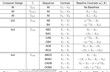
Next, Table 2.2 shows the optimal LCBs under these four considered structures. Derivation of
the optimal LCBs can be found in Appendix B.1. Note that sequence and subject subscripts are
dropped. Additionally, Table 2.2 shows the within-subject contrast that corresponds to the expected
treatment effect,τA−τB. When the baselines and outcomes are ordered by treatment, this contrast
is alwaysYA−YB; when the baselines and outcomes are ordered by period, the contrast will differ
by sequence.
Compound Symmetry (CS) Covariance Structure
As previously shown for the 2×2 design (Mehrotra, 2014), the variance conditional on the LCB
(2.10) is
V(YiAk−YiBk|aTXik,ΣCS) = 2σ2(1−ρ)
for each considered uniform design. This is simply the variance ofYiAk−YiBkand thus there is no
LCB that improves the efficiency of the treatment estimate. If an LCB were included in the model, a
the efficiency of the inferential procedure. This effect would be most pronounced in small samples, a
frequent characteristic of crossover trials in practice. In general, when cov(YiAk−YiBk,aTXik) = 0
for allaT, there is no LCB that improves the efficiency of the treatment estimate.
Double Compound Symmetry (DCS)/ Equipredictability (EP) Covariance Structure
For any of the considered designs, the conditional variances (2.10) under DCS and EP are:
V(YiAk−YiBk|aTXik,ΣDCS) = 2σ2(1−ρ2)−
σ4(a1−a2)2(ρ1−ρ2)2
V(aTX
ik) V(YiAk−YiBk|aTXik,ΣEP) = 2σ2(1−ρ2)−
σ4(a
1−a2)2(ρ1−ρ3)2
V(aTX
ik)
Notably, whileV(aTXik)depends on the specific design,a?T = (1,−1,0, ...0)minimizes the
condi-tional variance in each case. Thus,aT?Xik=XiAk−XiBkis the optimal LCB when the underlying
covariance structure is DCS or EP. This result is also valid if we assume separate variances for the
baselines and outcomes (i.e. V(Xidk) =σX2,V(Yidk) =σY2, for alld). Next, to obtain an unbiased
estimate of τA−τB (Section 2.4), we either need to condition at the sample mean of the LCB,
1
n Ps
i(XiAk−XiBk), or shiftXiAk−XiBkby the sample mean and condition at zero. For simplicity,
we refer to this LCB asXA−XB.
Autoregressive(1) [AR(1)] Covariance Structure
The AR(1) structure is only sensible for a period-ordered model. In this setting, we assume that the
baselines/outcomes are ordered temporally and thus the within-subject contrast of interest differs
by sequence. Table 2.2 shows the LCBs that minimize the conditional variance of the treatment
effect for each sequence, under an AR(1) assumption. These optimal LCBs will simply be referred
to as the AR(1) covariate. For the2×2and3×3designs, the optimal LCBs in pairs of sequences
are just negatives of each other. The AR(1) covariate also depends on the AR(1) correlation,ρ. In
practice, ρwill need to be estimated to use the AR(1) covariate. In Section 2.5.3, we provide an
approach to estimateρ. Finally, to obtain an unbiased estimate of the treatment effect, we either
condition at the sample mean of the AR(1) covariate, or shift the AR(1) covariate by the sample
Table 2.2: Uniform Design: Optimal LCB by Design and Covariance Structure
Crossover Design Σ Sequence Contrast Baseline Covariate (aTi?X)
All ΣCS All YA−YB No Baselines
All ΣDCS All YA−YB XA−XB
All ΣEP All YA−YB XA−XB
2x2 ΣAR AB Y1−Y2 ρ−2X1−X2
BA Y2−Y1 −(ρ−2X1−X2)
3x3 ΣAR ABC Y1−Y2 X1−X3
BAC Y2−Y1 −(X1−X3)
CAB Y2−Y3 ρ−2X2−X3
CBA Y3−Y2 −(ρ−2X2−X3)
ACB Y1−Y3 X1+X2−cX3
BCA Y3−Y1 −(X1+X2−cX3)
4x4 ΣAR ABCD Y1−Y2 X1−X3
BDAC Y3−Y1 −(X1+X2−X3−X4)
CADB Y2−Y4 X2+X3−(1 +ρ2)X4
DCBA Y3−Y4 −(X3−ρ−2X4)
Notes: c = (1+ρ
2+ρ4)+√(1+ρ2+ρ4)2+4ρ2(1+ρ2)2
2(1+ρ2) . CS = Compound Symmetry; DCS = Double
Compound Symmetry; EP = Equipredictability; AR = Auto-regressive (1).
2.5.3. Adaptive Data-Based Approach
While the optimal LCB depends on the covariance structure, in practice the covariance structure is
unknown. This motivates a data-based adaptive approach that chooses an analytic strategy based
on the most likely covariance structure. Our adaptive approach, which is similar to Mehrotra’s
Method X (Mehrotra, 2014), is as follows:
1. For the given data set, fit four models of the treatment ordered baselines and measurements
where Σ = V(Zik) is assumed to be CS, EP, DCS, or UN (unstructured) and one model
where the temporally ordered baselines/outcomes are assumed to follow an AR(1) covariance
structure. All models use a saturated means model for the combined vector of baselines and
outcomes
2. Obtain the corrected Akaike Information Criterion (AICC) for each model. AICC is a small
sample correction of AIC (Hurvich and Tsai, 1989).
3. UseXA−XB as the LCB except when (1) the AICC is smallest under CS; in this case use
(Table 2.2)
4. Fit the appropriate regression model based on the covariate choice from Step 3. If the AR(1)
covariate is chosen, then estimateρbased on the AR(1) model from Step 1.
We did not derive an LCB for UN, since this result rapidly becomes complex with increasing number
of periods. However, given (2.9) and (2.13), reductions in the conditional variance can be obtained
by including XA −XB as a covariate. In Chapter 3 we derive the optimal LCB under an UN
covariance for a 2-period design.
2.6. Application to Data Analysis
In this section, we apply the methods to two real data sets, one each from a 2 ×2 and 3×3
crossover design. For each data example, we consider the results obtained using each of the
variance-minimizing LCBs described in Table 2.2, using no baselines, the adaptive method, and
where change from baseline (CFB) scores are used as the outcome (and no baselines are included
as covariates in the model). CFB is widely used in practice and is a natural benchmark for
com-parison of our proposed methods. As is typically done (Jones and Kenward, 2003), our CFB model
includes random subject effects and fixed effects for period and treatment. Note that by assuming
random subject effects, the underlying covariance structure of the CFB outcomes is assumed to be
CS. Table 2.3 (2×2design) and Table 2.4 (3×3design) show the estimated unstructured
covari-ance matrix of the treatment ordered baselines and outcomes, the adaptive AICC results, and the
treatment effect estimates, standard errors, and p-values for all considered methods.
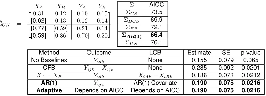
2.6.1. Real Data Example I:2×2Crossover Design
In this example (previously published as Example 2 from Mehrotra, 2014), a biomarker associated
with renal function was measured for each of 20 subjects at baseline and after treatment in a2×2
(AB/BA) crossover trial. The estimated treatment-ordered UN covariance matrix appears in Table
2.3; the upper left-hand corner corresponds to the estimates ofΣXX, the lower right toΣY Y and
the upper right toΣXY. For this example, the AICC favored the AR(1) structure. Notably, the CS
structure had the largest AICC relative to DCS, EP, and AR(1). This result suggests that using an
LCB should improve the efficiency of the estimate, and indeed, the SEs and the p-values using
adaptive method uses the AR(1) covariate. However, while the adaptive method chooses the AR(1)
covariate overXA−XB, the two LCB’s yielded very similar results. Lastly, we note that the CFB
approach, relative to the AR(1) covariate andXA−XB, yielded a larger estimated effect and SE,
but a similar p-value.
Table 2.3: Uniform Design Baseline Models:2×2Real Data Example I (N=20)
ˆ ΣU N =
XA XB YA YB
0.31 0.12 0.19 0.15
[0.62] 0.13 0.12 0.14
[0.77] [0.59] 0.21 0.14
[0.59] [0.86] [0.70] 0.20
Σ AICC
ΣCS 73.5
ΣDCS 69.9
ΣEP 72.1
ΣAR(1) 66.4 ΣU N 76.1
Method Outcome LCB Estimate SE p-value
No Baselines Yidk None 0.155 0.079 0.065
CFB Yijk−Xijk None 0.235 0.092 0.0201
XA−XB Yidk XiAk−XiBk 0.186 0.073 0.0212
AR(1) Yijk AR(1) Covariate 0.190 0.075 0.0216
Adaptive Depends on AICC Depends on AICC 0.190 0.075 0.0216
Notes:ΣˆU Nis the estimated unstructured covariance matrix of the treatment ordered responses. [] refer to correlation
es-timates. AICC values for the joint vector of responses under the various covariance structures are displayed. CFB=Change from Baseline. Method AR(1) refers to the covariates derived in Table 2.2 under AR(1). The adaptive method, based on the AICC values, chooses between methods No Baselines,XiAk−XiBk, and Method AR(1). CS = Compound Symmetry;
DCS = Double Compound Symmetry; EP = Equipredictability; AR = Auto-regressive (1); UN=Unstructured.
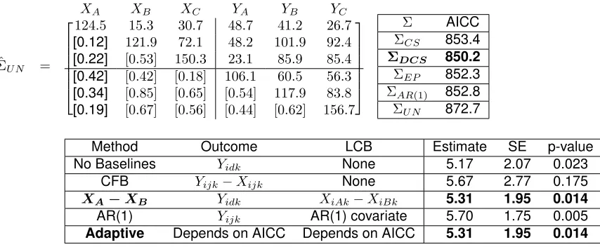
2.6.2. Real Data Example II:3×3Crossover Design
The following example is available online at http://www.stat.ufl.edu/CourseINFO/STA6167/
crossoverSFLM.pdf. This example contains data from a study which compared the effects on
heart rate of three treatments: a test drug, a standard drug, and a placebo. These treatments were
assigned to the six possible sequences, with four subjects in each sequence (N=24 total). For each
of the three visits and for each subject, heart rate was measured one hour following administration
of treatment. We illustrate the standard treatment compared to the placebo, but other pairwise
comparisons show similar results.
The estimated covariance matrix under UN appears in Table 2.4. We note that for this example,
cor-relations between different baselines and outcomes designated by the same treatment (or period)
tend to have higher correlations than those from different treatments (or periods). In this example,
com-pared to DCS, EP, and AR(1). This suggests that using an LCB should improve the efficiency of the
estimate. Indeed, relative to no baselines, the SEs and p-values using eitherXA−XBor the AR(1)
covariate are reduced. Here the adaptive approach would chooseXA−XAas the LCB covariate.
Lastly,XA−XBhas a noticeably lower SE and p-value than CFB, but has a slightly higher SE and
p-value than the AR(1) covariate.
Table 2.4: Uniform Design Baseline Models: 3×3Real Data Example (N=24)
ˆ ΣU N =
XA XB XC YA YB YC
124.5 15.3 30.7 48.7 41.2 26.7
[0.12] 121.9 72.1 48.2 101.9 92.4
[0.22] [0.53] 150.3 23.1 85.9 85.4
[0.42] [0.42] [0.18] 106.1 60.5 56.3
[0.34] [0.85] [0.65] [0.54] 117.9 83.8
[0.19] [0.67] [0.56] [0.44] [0.62] 156.7
Σ AICC
ΣCS 853.4
ΣDCS 850.2
ΣEP 852.3
ΣAR(1) 852.8
ΣU N 872.7
Method Outcome LCB Estimate SE p-value
No Baselines Yidk None 5.17 2.07 0.023
CFB Yijk−Xijk None 5.67 2.77 0.175
XA−XB Yidk XiAk−XiBk 5.31 1.95 0.014
AR(1) Yijk AR(1) covariate 5.70 1.75 0.005
Adaptive Depends on AICC Depends on AICC 5.31 1.95 0.014
Note:ΣˆU N is the estimated unstructured covariance matrix of the treatment ordered responses. [] refer to correlation
esti-mates. AICC values for the joint vector of responses under the various covariance structures are displayed. CFB=Change from Baseline. Method AR(1) refers to the covariates derived in Table 2.2 under AR(1). The adaptive method, based on the AICC values, chooses between methods No Baselines,XiAk−XiBk, and Method AR(1). CS = Compound Symmetry;
DCS = Double Compound Symmetry; EP = Equipredictability; AR = Auto-regressive (1); UN=Unstructured.
2.7. Simulations
The simulation study was designed to answer the following questions: (1) Is the Type I error rate
maintained, both for the two benchmarks (no baselines and CFB), for each of the LCB’s under the
correct covariance structure and when the covariance structure is misspecified, and for the adaptive
method; (2) When the LCB is optimal for the underlying covariance structure, does including the
optimal LCB offer an increase in power over the benchmarks; (3) Does the adaptive method capture
any power gains seen by using the optimal LCB under the correct covariance structure; and (4) Is
there any overall recommendation that can be made for practioners?
We simulated 20,000 trials for a variety of scenarios. The number of simulated data sets is rather
inflation. The simulation scenarios were defined by the hypotheses (null,τA−τB = 0; alternative,
τA−τB 6= 0), Σ(CS, DCS, EP, AR(1), UN), average pairwise correlation (ρ¯), and sample sizes.
Hypothesis tests were used with a nominal type I error rate of 0.05. Response vectors for each
subject within each simulated trial were generated from a multivariate normal with a
sequence-invariant Σ; either CS, DCS, EP, or AR(1) as described in Table 2.1, or UN under a treatment
ordering (Equations 2.5,2.6). Throughout we assumed a common varianceσ2 = 1andρ¯≈0.60.
For all designs: under CS,ρ= 0.6; under EP,ρ2= 0.60,ρ1= 0.70,ρ3= 0.50. DCS, AR(1), and UN
correlations vary by design (see Appendix B.2).
Under CS, DCS, EP, and UN, the response vector was generated under a treatment ordering,
based on the mean models in (2.3, 2.4) with γid = 0 for all d. For2 ×2, we set µ = 6.5 and
E(Xidk) = ζid = 0.5 such that E[(XA, XB, YA, YB)T] = (0.5,0.5,6.5 +τA,6.5 +τB)T; for3×3, µ= 7andE(Xidk) = 1such thatE[(XA, XB, XC, YA, YB, YC)T] = (1,1,1,7 +τA,7 +τB,7 +τC)T;
for 4 ×4, µ = 7.38 and E(Xidk) = 1.375 such that E[(XA, XB, XC, XD, YA, YB, YC, YD)T] = (1.375,1.375,1.375,1.375,7.38 +τA,7.38 +τB,7.38 +τC,7.38 +τD)T. Under AR(1), the response
vector is defined based on the period ordered mean models (2.12). See the Appendix for the
specific parameter values. For 2×2, E[(X1, Y1, X2, Y2)T] = (0,6 +τd[i,1],1,7 +τd[i,2])T; for 3×
3, E[X1, Y1, X2, Y2, X3, Y3)T] = (0,6 + τd[i,1],1,7 + τd[i,2],2,8 + τd[i,3])T; for the 4 ×4 design,
E[(X1, Y1, X2, Y2, X3, Y3, X4, Y4)T] = (0,6 +τd[i,1],1,7 +τd[i,2],2,8 +τd[i,3],2.5,8.5 +τd[i,4])T. Under the null,τA=τB = 0(andτC=τD = 0as appropriate), while under the alternative, for each
sce-nario,τA−τB was fixed such that using the no baselines model yielded 80% power (see Appendix
B.2). For the3×3and4×4design,τC−τB andτD−τB (4×4only) were set equal toτA−τB.
As expected, estimates ofτA−τBwere approximately unbiased for all methods under all scenarios
(results not shown). Power results are shown for the2×2(Table 2.5),3×3(Table 2.6), and4×4
designs (Table 2.7), with indications of where type I error inflation occurs, while type I error results
for all designs can be found in Appendix B.3. Lastly, while our CFB model used random subject
effects (and thus assumed a CS structure), power results were comparable to when we used a CFB
model with an unstructured covariance structure.
2.7.1. 2×2Crossover Design: Simulation Results
The type I error was maintained across all simulations when baselines were excluded from the
28), particularly under AR(1). This is most likely due to how the CFB method assumes that the
CFB outcomes follow a CS covariance structure. As we pointed out earlier, misspecifying the
covariance structure in a mixed model can lead to type I error inflation, regardless of sample size
(Gurka, Edwards, and Muller, 2011). Type I error inflation was rare whenXA−XB was included
as the LCB, but including the optimal LCB under AR(1) yielded type I error inflation at smaller
sample sizes. Lastly, the adaptive method exhibited type I error inflation at the lower sample sizes,
especially under DCS, EP, and AR(1). As to why the adaptive method inflates the type I error,
the adaptive method’s success rate, or how often the AICC correctly picks the ”right” covariance
structure gives us some insight. For the 2×2 design, especially at small sample sizes, there
is insufficient information to accurately choose the correct structure and the AICC criterion has
difficulty picking the ”correct” covariance structure (and thus the optimal LCB). Further, from our
simulations, we found that when the incorrect covariance structure was chosen, the standard error
of the treatment effect estimate was often deflated, leading to the inflated type I error.
Compared to the benchmarks (no baselines or CFB), including the optimal LCB increased power
for both DCS and EP. Similarly, using no baselines under a CS structure yielded the most power
and largely outperformed CFB. Under an AR(1) structure, the optimal LCB increased power at
sample sizes greater than 20, but could not be evaluated at smaller sample sizes due to type I error
inflation. In general, the adaptive method captured the power gains seen by using the optimal LCB,
and it also matched the highest power observed using XA−XB under an unstructured matrix.
However, as mentioned above, at smaller sample sizes, the adaptive method often suffers from
type I error inflation. Despite this, for N≥ 28, we see that the adaptive method does not suffer
from any type I error inflation, suggesting that this method could be used for larger sample sizes.
Overall, given that the adaptive method does not maintain the type I error in a variety of scenarios,
our recommendation for a2×2design is to useXA−XB as a covariate. This method consistently
outperformed CFB and uniformly did well across all the covariance structures.
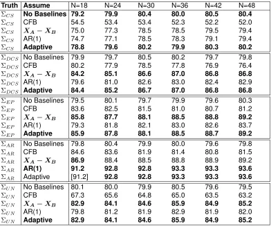
2.7.2. 3×3Crossover Design: Simulation Results
With the exception of the adaptive method at N=18 under AR(1) and CFB under UN, all methods
maintained the type I error. The lack of type I error inflation for the adaptive method can be attributed
to the high success rate of the AICC criterion in the3×3design. For example, at N=18 under EP,
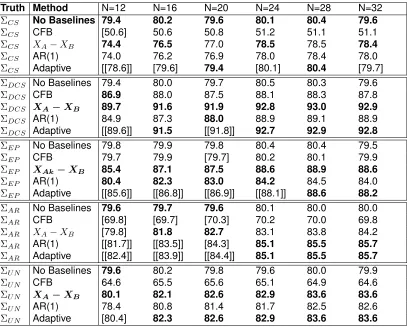
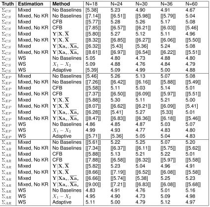
Table 2.5: 2×2Simulations: Under the Alternative Hypothesis, Power
Truth Method N=12 N=16 N=20 N=24 N=28 N=32
ΣCS No Baselines 79.4 80.2 79.6 80.1 80.4 79.6
ΣCS CFB [50.6] 50.6 50.8 51.2 51.1 51.1
ΣCS XA−XB 74.4 76.5 77.0 78.5 78.5 78.4
ΣCS AR(1) 74.0 76.2 76.9 78.0 78.4 78.0
ΣCS Adaptive [[78.6]] [79.6] 79.4 [80.1] 80.4 [79.7]
ΣDCS No Baselines 79.4 80.0 79.7 80.5 80.3 79.6
ΣDCS CFB 86.9 88.0 87.5 88.1 88.3 87.8
ΣDCS XA−XB 89.7 91.6 91.9 92.8 93.0 92.9
ΣDCS AR(1) 84.9 87.3 88.0 88.9 89.1 88.9
ΣDCS Adaptive [[89.6]] 91.5 [[91.8]] 92.7 92.9 92.8
ΣEP No Baselines 79.8 79.9 79.8 80.4 80.4 79.5
ΣEP CFB 79.7 79.9 [79.7] 80.2 80.1 79.9
ΣEP XAk−XB 85.4 87.1 87.5 88.6 88.9 88.6
ΣEP AR(1) 80.4 82.3 83.0 84.2 84.5 84.0
ΣEP Adaptive [[85.6]] [[86.8]] [[86.9]] [[88.1]] 88.6 88.2
ΣAR No Baselines 79.6 79.7 79.6 80.1 80.0 80.0
ΣAR CFB [69.8] [69.7] [70.3] 70.2 70.0 69.8
ΣAR XA−XB [79.8] 81.8 82.7 83.1 83.8 84.2
ΣAR AR(1) [[81.7]] [[83.5]] [84.3] 85.1 85.5 85.7
ΣAR Adaptive [[82.4]] [[83.9]] [[84.4]] 85.1 85.5 85.7
ΣU N No Baselines 79.6 80.2 79.8 79.6 80.0 79.9
ΣU N CFB 64.6 65.5 65.6 65.1 64.9 64.6
ΣU N XA−XB 80.1 82.1 82.6 82.9 83.6 83.6
ΣU N AR(1) 78.4 80.8 81.4 81.7 82.5 82.6
ΣU N Adaptive [80.4] 82.3 82.6 82.9 83.6 83.6
Notes: Values (Power %) are shown in bold if method yields the highest or second highest power in that sample size/covariance structure combination without type I error inflation. Entries are in brackets/double brackets if under the same scenario, but under the null hypothesis, the type I error is two/three SE’s above 5% (>5.31%,>5.46%) based on 20,000 simulations. CFB=Change from Baseline. Method AR(1) refers to the covariates derived in Table 2.2 under AR(1). The adaptive method, based on AICC values, chooses between methods No
Base-lines,XA−XB, and Method AR(1). CS = Compound Symmetry; DCS = Double Compound Symmetry; EP =
Equipredictability; AR = Auto-regressive (1); UN=Unstructured.
simulations).Next, compared to the benchmarks (no baselines and CFB), the optimal LCBs led to
increased power under all scenarios. Furthermore, the adaptive method captured these power
gains (superior to the benchmarks) by using the optimal LCBs and also matched the highest power
observed usingXA−XB under UN. Coupled with the fact that the adaptive method did not suffer
from type I error inflation, the adaptive method could be used for3×3crossover design.
2.7.3. 4×4Crossover Design: Simulations
All methods maintained the type I error, except for CFB under UN. Like in the2×2design, the type
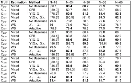
Table 2.6: 3×3Simulations: Under the Alternative Hypothesis, Power
Truth Assume N=18 N=24 N=30 N=36 N=42 N=48
ΣCS No Baselines 79.2 79.9 80.4 80.0 80.5 80.4
ΣCS CFB 54.5 53.4 53.4 52.3 52.2 52.0
ΣCS XA−XB 75.0 77.3 78.5 78.5 79.5 79.4
ΣCS AR(1) 74.7 77.1 78.5 78.3 79.1 79.4
ΣCS Adaptive 78.8 79.6 80.2 79.9 80.3 80.2
ΣDCS No Baselines 79.9 79.7 80.5 80.2 79.7 79.8
ΣDCS CFB 80.2 77.9 78.5 77.8 76.9 76.4
ΣDCS XA−XB 84.2 85.1 86.6 87.0 86.8 86.8
ΣDCS AR(1) 79.6 81.0 82.6 83.0 82.4 82.9
ΣDCS Adaptive 84.4 85.2 86.7 87.0 86.8 86.8
ΣEP No Baselines 79.5 80.1 79.7 79.9 79.6 80.3
ΣEP CFB 83.6 82.5 81.5 81.0 80.7 81.2
ΣEP XA−XB 85.8 87.7 88.1 88.5 88.8 89.2
ΣEP AR(1) 79.3 81.8 82.1 83.0 82.6 83.7
ΣEP Adaptive 85.9 87.8 88.1 88.5 88.7 89.2
ΣAR No Baselines 79.8 80.4 79.9 80.0 79.6 79.8
ΣAR CFB 84.6 83.6 81.9 81.4 80.8 81.5
ΣAR XA−XB 86.9 88.4 88.5 88.8 88.9 89.2
ΣAR AR(1) 91.2 92.8 92.8 93.3 93.3 93.6
ΣAR Adaptive [91.2] 92.8 92.8 93.3 93.3 93.6
ΣU N No Baselines 80.1 80.0 79.9 80.5 79.6 79.5
ΣU N CFB 67.3 65.6 64.8 65.0 63.5 63.2
ΣU N XA−XB 82.9 84.1 84.6 85.9 84.9 85.2
ΣU N AR(1) 79.8 81.2 81.9 82.9 81.9 82.0
ΣU N Adaptive 82.9 84.1 84.6 85.9 84.9 85.2
Notes: Values (Power %) are shown in bold if method yields the highest or second highest power in that sample size/covariance structure combination without type I error inflation. Entries are in brackets/double brackets if under the same scenario, but under the null hypothesis, the type I error is two/three SE’s above 5% (>5.31%,>5.46%) based on 20,000 simulations. CFB=Change from Baseline. Method AR(1) refers to the covariates derived in Table 2.2 under AR(1). The adaptive method, based on AICC values, chooses between methods No Baselines,XA−XB, and Method AR(1). CS = Compound Symmetry; DCS = Double
Compound Symmetry; EP = Equipredictability; AR = Auto-regressive (1); UN=Unstructured.
covariance structure. Importantly, the type I error was maintained for the adaptive method in all
scenarios. Like in the3×3design, the optimal LCBs outperformed both benchmarks (CFB and no
baselines) under all scenarios. Additionally, the adaptive method did approximately as well as the
optimal LCBs (and also beat out the benchmarks), while also matching the highest power observed
usingXA−XB under UN. Given this, along with the fact that the adaptive method does not suffer
from type I error inflation, the adaptive method could be used in the4×4crossover design, but with