Energy-Efficient Management
of UMTS Access Networks
Luca Chiaraviglio, Delia Ciullo, Michela Meo, Marco Ajmone Marsan
Electronics Department, Politecnico di Torino, Torino, Italy
Abstract—The increasing concern about the energy consump-tion of telecommunicaconsump-tion networks is driving operators to manage their equipments so as to optimize energy utilization without sacrificing the user experience. In this paper, we focus on UMTS access networks, since access devices are the main energy consumers in UMTS networks. We propose a novel approach for the energy-aware management of UMTS access networks, consisting in a dynamic network planning, that, based on the instantaneous traffic intensity, reduces the number of active access devices when they are underutilized (typically at night). When some access devices are switched off, radio coverage and service provisioning are taken care of by the devices that remain active, possibly with some small increase in the emitted power, so as to guarantee that service is available over the whole area, with the desired quality.
I. INTRODUCTION
ICT is becoming a major component of the energy con-sumption budget. Current estimates indicate that ICT is re-sponsible for a significant fraction of the world electricity con-sumption, ranging between 2% and 10% [1]. The main energy consumers in the ICT field are large data centers and server farms, and telecommunication networks, including wired and wireless telephony networks as well as the Internet. Both the networking equipment themselves, and the associated cooling systems are greedy energy consumers. In Italy, Telecom Italia, the main TELCO in the Country, consumes more than 2 TWh a year, representing about 1% of the total national electricity demand, second only to the national railway system [2]. The energy consumption of ICT is expected to grow even further in the future. Estimates forecast a ten-fold increase of the energy consumed by the telecommunication sector in Italy in the next ten years, the main culprit being customer premises networking equipment.
Telecommunication network operators have become very sensitive to the energy issue, since they view a reduction of the energy consumption of their networks as both a painless approach to cost reduction, and an important aspect for the promotion of their image in the media. For this reason, TEL-COs are studying different approaches to energy consumption reduction, including the introduction of the energy issue in the network design, planning, and management phases. In this paper we tackle the issue of energy-aware management of UMTS access networks.
Our energy-aware network management approach, that was first sketched in [3] consists in a dynamic network planning, that, based on the instantaneous traffic intensity, reduces the number of active access devices when they are underutilized,
e.g., during night periods in office areas. We focus on access devices, namely Base Transceiver Stations (BTS), or Node-B’s in UMTS jargon, since these are the main energy consumers in radio access networks [4]. When some Node B’s are switched off, radio coverage and service provisioning are taken care of by the devices that remain active, possibly with some small increase in the emitted power, so as to guarantee that service is available over the whole area. The switch-off of the access devices must be carefully decided, so as to maintain the desired quality of service (QoS) guarantees, and meet electromagnetic coverage constraints.
We start from a network where UMTS cells are dimensioned for electromagnetic coverage and for the desired QoS during the peak traffic period. We assume that dimensioning is essentially driven by traffic demands, as it normally happens in metropolitan areas, comprising a large number of small cells. This planning becomes excessive in the areas that for some time are subjected to a traffic much lower than the peak. During these periods it becomes possible to turn off some Node-B’s, provided that electromagnetic coverage is preserved. Generally, one or a few cells of a UMTS access network are served by one B. Turning off one Node-B implies the unavailability of the corresponding cells. We use a variation of traditional network planning schemes to identify the traffic level that allows turning off some Node-B still guaranteeing the QoS desired by the operator, as well as electromagnetic coverage. Once the switch-off traffic level is identified, it is possible to use the daily traffic profile in a given area to determine the length of the period in which the Node-B equipments can be switched off. This in turn determines the amount of energy that can be saved. Clearly, this approach is not feasible in areas with low traffic density and large cells, since radio coverage cannot be guaranteed if some cells are switched off.
We claim that it is possible to apply the schemes that we propose to a real urban UMTS access network, due to the fact that operators are now beginning to incorporate in their equipment new software features that allow network elements to be remotely controlled, and even switched off [5]. Considering the large number of access devices present in a typical national UMTS access networks, the total amount of energy saved by an operator implementing the proposed schemes can be huge, as we will show with some examples.
traffic classes, in this paper we better represent data traffic, with users generating sessions consisting of a series of elastic file transfers. Second, in this paper we explicitly consider three alternative approaches for the switch-off of Node-B’s. Finally, all numerical results presented in this paper are new, and refer to more realistic parameters.
II. UMTS RADIOACCESSARCHITECTURE
UMTS was designed as an evolution of the immensely successful GSM system, to carry many types of traffic, originating from real-time circuit-switched, or elastic packet-switched services, and offer higher data rates and a wide range of telecommunications services, including video calls and Internet access.
The UMTS architecture is typically composed by three interacting domains: User Equipments (UEs), Terrestrial Radio Access Network (UTRAN), and Core Network (CN). The UE is the mobile terminal carried by the end user. The UTRAN provides wireless connectivity between the UEs and the CN, that is the long distance network, which is mostly wired. Basically, the UTRAN consists of two types of elements: the Node-B, that is the network Base Transceiver Station (BTS), and the Radio Network Controller (RNC), that controls one or more Node-B’s. While Node-B and RNC can be co-located in the same device, typical implementations have a RNC located in a central office, and serving several Node-B’s.
As reported in [6], an individual UTRAN equipment con-sumes about 6 kW, including power amplifiers, digital signal processors, air-conditioning modules and feeders connecting the RNC to the Node-B. Considering only the Node-B, power consumption amounts to nearly 800 W [7] with the power needed to transmit from the antenna in the range 1-40 W. The large number of equipments in the UTRAN makes the total power consumed at the access network particularly significant: any reduction of power consumption in the Node-B or RNC translates into a significant reduction of the overall network power consumption. This is the reason why we focus on the possibility of turning off some Node-B’s during the periods in which the capacity they provide is redundant.
A. Link Budget and Propagation Model
The Node-B configuration defines the maximum allowed path loss, i.e., the maximum power reduction of the signal between UE and Node-B, which still guarantees a good quality communication.
The maximum path loss computation is based on typical link budget parameters; the main configuration parameters are shown in Table I for the Uplink (UL) direction and in Table II for the Downlink (DL) direction. For more details see [8]. The most critical parameter for the UL direction is the UE transmitted power,PU E. The DL direction limits the available
capacity of the cell, since the BTS transmitted power, PBS,
must be shared among all users.
After computing the allowed path loss, i.e., the maximum loss allowed considering both the UL and DL directions, we use the well-known Walfish-Ikegami propagation model [9]
to calculate the maximum cell radiusRmax. In this way, we
can verify that when some Node-B’s are switched off, the electromagnetic coverage of the service area is preserved, with the desired transmission quality.
TABLE I
MAINLINK-BUDGET PARAMETERS: UPLINK OF AMICROCELL
Voice Video Data
PU E [dBm] 21 24 24
AntennaGainM S [dB] 0 2 2
EB/N0 [dB] 5 2 1.5
P rocessingGain [dB] 25 18 14
T otalN oise [dB] -102 -102 -102
AntennaGainBS [dB] 15 15 15
DiversityGain [dB] 2 2 2
LN A [dB] 2 2 2
Sof tHODiversityGain [dB] 3 3 3
SlowF adingM argin [dB] 13.16 13.16 13.16
TABLE II
MAINLINK-BUDGET PARAMETERS: DOWNLINK OF AMICROCELL
Voice Video Data
PBS [dBm] 37-43 37-43 37-43
AntennaGainBS [dB] 15 15 15
EB/N0 [dB] 4 2.5 2
P rocessingGain [dB] 25 18 14
T otalN oise [dB] -99 -99 -99
AntennaGainM S [dB] 0 2 2
Sof tHODiversityGain [dB] 3 3 3
SlowF adingM argin [dB] 13.16 13.16 13.16
Note that we assume that Node-B’s are equipped with electronic tilting, so that antenna orientation modifications, necessary to increase the cell size, are possible. Also, in the computation of energy consumption, we neglect the possible transmission power increase in the uplink, since it is marginal with respect to the power needed for the access network devices. Moreover, since we are considering a urban scenario with small cells, the terminal lifetime is marginally affected by the limited cell size increase requested by our scheme.
III. THECELLMODEL
In order to model the behavior of the cells controlled by a Node-B, we have to consider both circuit-switched (CS, for short) voice and video services, and packet-switched (PS) data services. Based on the operator radio resource allocation strategies, the bandwidth is dynamically partitioned between the two classes of service. Usually, since CS services are the most remunerative, they can use as much bandwidth as needed, as far as a minimum amount of bandwidth, Bm, is reserved
to PS services; the bandwidth devoted to PS services cannot exceed a maximum amount BM. Since CS services have
many, they are small, and can be assumed to have similar size and traffic.
In the rest of this section, we first describe the model used for CS services, and then the model used for PS services. Both are simple models, adequate for a preliminary quantification of possible energy savings.
A. The Model for Circuit Switched Services
For CS services, we use a traditional simple teletraffic model based on Markovian assumptions for traffic processes; the model allows us to evaluate the cell performance in terms of blocking probability for a number of different service types.
The teletraffic model consists in a multi-class M/M/N/0 queue, that was widely used in the literature for cellular systems planning (see for example [10]). The model focuses on a single cell in a cellular system, approximating the interaction between neighboring cells through a simplified description of the flow of handovers.
In general, we consider K classes of service with different resource requirements. Each classicall requires an amount of bandwidth equal toCi.
We adopt the following simple traffic assumptions:
• users generate classicalls according to a Poisson process
with rate λi;
• incoming handovers for class i calls occur according to
a Poisson process with parameter λh,i;
• no queuing is possible; calls are blocked if the available
bandwidth is not sufficient to satisfy an incoming request;
• the service time for a classicall is distributed according
to an exponential probability density function (pdf) with mean 1/µi;
• the time spent by the user in the cell is distributed
according to an exponential pdf with mean 1/µh.
The traffic model is extremely simple, (we neglect, for exam-ple, the fact that capacity depends by the position of active users’ location) but adequate for a first estimation of the amount of energy saving that can be obtained with energy-aware network management algorithms.
The cell is described by the numbers of active calls in each class, ni for class i, collected in the vector s =
(n1, n2,· · ·, nK). The model state space, i.e., the set of all
possible states, is given by
S={s= (n1, n2,· · ·, nK)| K
X
i=1
Cini≤CT} (1)
where CT is the total bandwidth available for CS services.
Denoting by A the total UMTS capacity (i.e., the maximum data rate), CT = A −Bm, where Bm is the minimum
bandwidth reserved to PS services.
From well-known queueing theory results, we know that the
steady-state probabilities for this model are:
π(s) =π(n1, n2,· · ·, nK) = K
Y
i=1 ρni
i
ni!
X
s∈S K
Y
i=1 ρni
i
ni!
(2)
where ρi = (λi+λh,i)/(µi+µh)is the class i traffic load.
The interaction between neighboring cells, that is represented by the parameter λh,i, is derived by a fixed-point iterative
procedure, in such a way that, at steady-state, the incoming and outgoing handover flows are equal.
The blocking probability for class i calls is given by the probability of the states in which an additional class i call cannot be accepted due to lack of available bandwidth:
Pb,i=Ps∈Siπ(s) with Si={(n1, n2,· · ·, nK)|CT−Ci<
PK
i=1Cini≤CT}(3)
The average number of active classicalls is:
E[Ai] =
X
s∈S
niπ(s) (4)
The typical CS applications supported by UMTS are voice and video, as reported in [11], with rates, respectively, equal to 12.2 Kbit/s, and 64 Kbit/s. Thus, we considerK= 2classes of circuit-switched service, with those capacity requirements. The mean call duration, 1/µi, is set according to typical
values used in the literature [12]: 3 minutes for voice, and 5 minutes for video. The UMTS maximum transfer rate A is 2 Mbit/s; the minimum bandwidth reserved to PS services is taken to be Bm = 144 Kb/s, and CT = A−Bm. The
value of µh depends on user mobility; given the cell radius
R, by assuming a triangular pdf of speed, with averageV, and support in[0,2V],µh results
µh=V /(4R)ln(2) (5)
In the rest of this paper we consider an average speed V equal to10m/s, i.e., about 36 km/h. Although this value may be somewhat high, it should be noted that reducing the user mobility implies a lower number of handovers, hence a lower call blocking probability. Thus, a higher mobility represents a conservative assumption for our scenario.
B. The Model for Packet Switched Services
UMTS PS services, typically web browsing, and other Internet-related applications, are provided by making data connections share the available bandwidth. As previously men-tioned, based on the number of active CS calls, the available bandwidth B varies between a minimum value, Bm, and a
maximum value,BM, with a granularity that depends on the
UMTS code allocation mechanisms. As an approximation, we assume that just two bandwidth values are possible; namely, Bm= 144Kbit/s and BM = 384Kbit/s.
assume that during the lifetime of a data connection, the PS bandwidth B remains constant. Therefore, we separately model the two cases with B = Bm and B = BM; we
then combine the results of the two models, based on the steady-state probabilities of the number of active CS calls, that actually decide the PS available bandwidth.
Model: We assume that a PS call, basically a web browsing session, consists of a bunch of data transfers (or data connec-tions) generated in a short time. Since we expect that most of the traffic flows in the downlink direction, we actually model the PS traffic in the downlink. Each time a new session starts, a data connection begins; a session ends when its last data connection ends. We assume that no more thanSsessions can be active at the same time in the cell. Active data connections are elastic and fairly share the available bandwidth; no more than D data connections can be admitted in the cell. We also assume that if a data connection is not admitted, its session is interrupted. Relying on the Markovian assump-tions listed below, our model consists of a MMPP/M/1/D-PS queue (a single-server Processor Sharing queue, with Markov-Modulated Poisson arrival process, Markovian service times, and finite capacity):
• New sessions are generated according to a Poisson
pro-cess with rate λs.
• While active, a session generates data connections
ac-cording to a Poisson process with rateγ; whenasession are active the total arrival rate is aγ.
• The number of data connections generated by a session is
geometrically distributed with parameterβ; i.e., the mean number of data connections per session is 1/(1−β).
• The amount of information transferred during a data
connection is exponentially distributed with mean value G; then, the duration of a connection served at bandwidth B (when there are no other active connections to share the bandwidth with) is exponentially distributed with parameterδ=B/G.
We solve the queue by modeling it as a continuous-time Markov chain (CTMC). Let the state variable be given by v = (s, d), where s is the number of active sessions, and d is the number of active data connections. The variable s is the state variable for the MMPP; drepresents the number of customers in the queue. The model state space, i.e., the set of all possible states, is given by
V ={v= (s, d)|0≤s≤S, 0≤d≤D} (6) Table III reports the possible CTMC transitions from the generic state (s, d): for each transition, the destination state, the transition rate, and the condition over (s, d) for the transition to be possible are indicated; the first column of the table hints also to the physical phenomenon that determines a given transition. We denote the steady-state probabilities by ω(v), orω(s, d).
As performance indices, we can evaluate the fraction of data connections that are rejected because the queue is full, that is derived as the ratio of the number of rejected connections in
TABLE III
PACKET-SWITCHED SERVICE: CTMCTRANSITIONS FROM STATE(s, d)
Phenomenon Destination Rate Condition New session (s+ 1, d+ 1) λs d < D,s < S New connection
admitted (s, d+ 1) sγ d < D,s >0 not admitted (s−1, d) sγ d=D,s >0
Connection ends
not the last one (s, d−1) δβ d >0,s >0
last one (s−1, d−1) δ(1−β) d >0,s >0
the time unit over the number of generated connections:
Ld=
PS−1
s=0 (sγ+λs)ω(s, D) +Sγω(S, D)
PS−1
s=0 λs+P S s=0
PD
d=0ω(s, d)sγ
(7)
(notice that we assume that a session that is not admitted does not generate a connection). Similarly, the fraction of sessions that are rejected is given by:
Ls=
PD
d=0ω(S, d)λs
λs
(8)
The average number of active sessions and connections are respectively given by:
Es=
X
v∈V
sω(s, d) Ed=
X
v∈V
dω(s, d) (9) For the numerical results presented in the rest of the paper, we use S = 50, D = 10, a mean amount of information to transfer with a data connection equal toG= 48KB, andδ=
B/G, the mean number of connections per session,1/(1−β)
equal to 10.
Interaction with the CS service model: As previously dis-cussed, the different time scales of CS and PS services allow us to assume that the available bandwidth is constant during a PS connection lifetime. Thus, we separately model the case in which the PS bandwidth isBm, orBM, and we compute the
performance indices as in (7), (8) and (9). LetL(m)d andL
(m)
s
be the indices for the caseB =Bm, andL
(M)
d andL
(M)
s for
the caseB =BM.
The average fraction of data connections that are not admit-ted is given by:
L∗ d=L
(m)
d P rob{B=Bm}+L
(M)
d P rob{B=BM} (10)
where P rob{B =Bi} denotes the probability that the
avail-able bandwidth isBi. The average fraction of rejected sessions
is:
L∗
s=L(m)s P rob{B=Bm}+L(M)s P rob{B=BM} (11)
The average number of active sessions and connections can be derived similarly.
In order to derive P rob{B =Bm} and P rob{B =BM}
we use the steady-state probabilities of the CS model from (2). The PS available bandwidth isBM if the CS connections
use an amount of bandwidth smaller than A−BM, with A
the total bandwidth of the cell,
P rob{B=BM}=Ps∈SMπ(s) with SM ={(n1, n2,· · ·, nK)|P
K
and
P rob{B=Bm}= 1−P rob{B=BM} (13)
IV. SWITCH-OFFSCHEMES
In this section, we describe a procedure to verify the feasibility of a Node-B switch-off scheme and to compute the possible power consumption reduction.
We consider a set of cells with the same radius R and the same traffic load. Radio coverage and cell dimensioning are typically performed so as to satisfy QoS constraints under peak traffic conditions; e.g., at peak traffic, the blocking probability for each class of calls must be smaller than a target valuePb(T). However, during off-peak periods, the system is probably overprovisioned and may waste a significant amount of power. Thus, our objective is to switch off some Node-B’s when the load in the corresponding cells is low: we have to decide the number of Node-B’s to switch off, and the load conditions under which Node-B switch-off is possible. These decisions are critical and should take into account two aspects. First, the cells that are not switched off must provide radio coverage over the whole area (including the portions that were covered by the switched off cells), and, in order to increase their radius, cells could require additional transmission power. Second, the larger cell radius induces also traffic increase, under which, QoS constraints must be guaranteed. The procedure we propose for cell switch-off is discussed below, and sketched in Fig. 1. LetΛ(t)be the time-varying function of the new call gen-eration rate, which we partition into service classes according to some constantsαi; in other terms, the time varying classi
call arrival rate is Λi(t) = αiΛ(t). The functionsΛi(t)have
the typical periodic night/day pattern, such as those reported in Fig. 31. Let Coff and Con be the number of cells that, respectively, are switched off and remain on, during low traffic periods (say, nights); xis the scaling factor Coff/Con, which represents the number ofoffcells for each cell that remainson. In order to cover the area left by offcells, theoncells radius must increase from R to R′ =kR, with k
depending on the cell geometry. At instant t, in normal conditions, the traffic is given by λi= Λi(t); whenCoff cells are switched off, the traffic in theoncells becomesλ′
i= (x+1)λi; correspondingly,
the load is ρ′ i= (λ
′ i+λ
′
h,i)/(µi+µ′h), withµ ′
h given by (5)
substitutingR′
toR, andλ′
h,iderived from the handover flow
balance iterative procedure.
We call night zone the time period during which we can switch off some cells, while still satisfying QoS guarantees. Clearly, the longer the nigh zone is, the higher is the power saving that can be achieved. The night zone is defined by the largest value of Λ(t)′ = (x+ 1)Λ(t)
that guarantees that blocking probability is smaller than Pb(T) for each service
class. The corresponding value of t, namelyt∗
, such that
Pb,i((x+ 1)Λi(t ∗
))≤Pb(T) ∀i (14)
1Actually, real traffic patterns have more complex periodic behaviors, but
in order to prove that significant energy savings are achievable, a simple sinusoidal behavior is enough.
Fig. 1. Procedure to verify a switch-off scheme.
plays a role similar to the peak hour used for dimensioning the system; traffic int∗
is the peak traffic of the night configuration withCon on cells. Let the average number of active calls at timet∗
be denoted byE[Ai](t∗). Given the total BTS power
PBS, we define the power per connection as:
Pconn=PBS/E[Ai](t∗) (15)
and use it in the link budget and in the Walfish-Ikegami attenuation model to find the maximum cell radius Rmax.
If Rmax > R′, the switch-off scheme can be implemented
without increasing the powerPBS. Otherwise, a new value for
the base station transmission power must be computed,P′ BS,
and electromagnetic exposure limits as described in [13] must be verified. If exposure limits are guaranteed, the scheme is feasible, and power consumption reduction can be computed from the value of P′
BS and the extension of the night zone.
Otherwise, if either exposure limits cannot be guaranteed, or no nigh zone is possible with constraint (14), a new scheme with a smaller number ofCoff cells should be assumed.
Once the Node-B’s to be switched off have been identified, the question arises about how to implement switch-off. Of course, it is not possible to just switch off the Node-B, since, even if the traffic is low, a number of users may be accessing the Node-B with their terminals for voice, video or data services.
In this paper we consider three different possibilities.
1.After the switch-off decision is taken, the network waits until no user is accessing the Node-B, which is thus switched off only when idle. This is the least invasive approach for users, but an obvious drawback is that the time between the switch-off decision and the Node-B idling may be long, thus limiting the effectiveness of the energy saving approach.
between the switch-off decision and the actual switch-off is less than in the previous case, but still significant, coinciding with the longest residual time of the services in progress at the time of the decision.
3. Immediately after the switch-off decision is taken, users are forced to implement a handover from the Node-B that is going to be switched off to one of the Node-B’s that remain active. This is the most invasive approach for users, but forced handovers are foreseen by UMTS standards, and thus the algorithm is well within the possibilities of present UMTS equipment. Actually, forced handovers are already used by operators, whenever some special maintenance must be implemented at a Node-B. The important advantage of this approach lies in the fact that the time between the switch-off decision and the actual switch-off can be controlled by the operator, and kept very low, so as to maximize the energy reduction effect.
Our numerical experiments, whose results are reported in the next session, indicate that, for the scenarios that we have examined, the first alternative is impractical, since the delay between the switch-off decision and the actual switch-off is excessively long. Instead, the other two options provide com-parable power savings. Some numerical data will be presented and discussed in the section that follows.
V. NUMERICALRESULTS
In this section we discuss some numerical results, to show that the power savings generated by the proposed access network management scheme can be huge.
We start with a simple uniform access network config-uration, where all cells are equal, discussing in detail the case in which one Node-B is switched off for every pair, and summarizing results for other configurations in which the fractions of Node-B’s that are switched off is larger. We then turn our attention to a hierarchical cellular structure, in which one umbrella cell overlaps with six microcells.
A. Uniform Scenario
We first consider a uniform scenario composed of many identical microcells (µ-cells) arranged in a grid, each cell corresponding to one Node-B. Eachµ-cell has radiusR= 100
m and total power PBS = 5W. The QoS target in each cell
is Pb(T) = 1% for voice calls; this blocking probability is
considered mandatory for telephony only, while other services can have, for short time periods, larger blocking probability.
We consider a switch-off configuration where oneµ-cell in each pair is switched off during the night zone, so thatx= 1; this scheme is represented by the top left scheme of Fig. 2. The radius ofoncells doubles during the night zone, becoming R′
= 200 m, and the call generation rate doubles as well. The functions Λi(t) (call generation rates) are reported
in Fig. 3 for two consecutive days: they have the simple sinusoidal shape that we assume for night/day patterns. The ratio between the peak and the minimum is about 17.
Fig. 4 reports the blocking probabilities perceived by each class of service during the two-day period. The night zone ex-tends from about 20:45 to 07:15; the extremes of this interval
Fig. 2. Possible switch-off configurations.
1e-05 0.0001 0.001 0.01 0.1 1
8:00 16:00 24:00 8:00 16:00 24:00 8:00
λ
Time [h]
Night zone Night zone
VOICE VIDEO DATA
Fig. 3. Call generation rates versus time in aµ-cell.
(that are the discontinuity points in the curves) correspond to the points in which the blocking probability for voice calls reaches 1% or, in other terms, are the peak hour traffic for the night scenario. The blocking probability for voice calls is always below the target; the maximum is achieved at peak traffic in the day and night hours. A similar behavior is shown by the average number of active calls that is reported in Fig. 5. The maximum cell radius computed from the propagation and link-budget models under traffic Λi(t)′ is reported in
Fig. 6. Focusing on voice traffic, without changing the base station transmitted power, the maximum cell radius is larger than 200 m from about 21:15 to 06:45, which is a smaller interval than the night zone identified by the QoS constraint. This means that we have two possibilities: we either reduce the night zone to the interval between 21:15 and 06:45, and leave the transmitted power unchanged, or we use the larger night zone between 20:45 and 07:15, but increase the transmitted
1e-10 1e-08 1e-06 0.0001 0.01 1
8:00 16:00 24:00 8:00 16:00 24:00 8:00
Pb
Time [h]
λ 2λ λ 2λ
VOICE VIDEO DATA
0.001 0.01 0.1 1 10 100 1000
8:00 16:00 24:00 8:00 16:00 24:00 8:00
E[call]
Time [h]
λ 2λ λ 2λ
VOICE VIDEO DATA
Fig. 5. Average number of active calls versus time.
140 160 180 200 220 240 260 280 300 320
8:00 16:00 24:00 8:00 16:00 24:00 8:00
Rmax
[m]
Time [h]
Night zone Night zone VOICE
VIDEO DATA
Fig. 6. Maximum cell radius achievable when half of the cells are off.
power in the intervals [20:45,21:15] and [06:45,07:15]. Notice that at the extremes of the night zone, when traffic is relatively high, the link budget is such that, at the cell border, data connections cannot obtain 144 Kb/s; however, we neglect this aspect since, even in normal situations, operators do not guarantee the highest bit rates at the cell border.
By leaving the transmitted power unchanged, every Node-B can be switched off for about 9.5 hours, thus saving 39.6%
of the power consumed in a day. The potential saving is 800
W × 9.5 h = 7.6 KWh. Since one out of two Node-B’s is switched off, the power saving is about 20% of the access network requirements.
This power saving is achievable if Node-B’s are switched off as soon as the traffic level and the transmission parameters allow it. As we discussed in Section IV, this is possible if users are forced to implement a handover from the B that is going to be switched off to one of the Node-B’s that remain active. If, instead, Node-Node-B’s are switched off only after all services in progress at the time of the switch-off decision terminate, but no new call is accepted, the saving is reduced. In Fig. 7, the curve labeled uniform
shows the distribution of the time required to reach the idle state for Node-B’s, obtained from the transient solution of the Markovian model described in Section III; we consider the model of circuit-switched services only, since the time to complete data connections is much smaller (the mean time to empty the data connection queue is upper bounded by 30 s). We can see that the cell is emptied with 90%probability after
0 0.1 0.2 0.3 0.4 0.5 0.6 0.7 0.8 0.9 1
0 500 1000 1400
CDF
Time to reach (0,0) [s] Uniform Scenario
Hierarchical Scenario
Fig. 7. CDF of the time to reach state(0,0).
about 20 minutes. This further reduces the switch-off time to 9.2 hours, so that the power saving is about 19%of the access network requirements.
While this power saving reduction can be negligible, the approach that simply waits for the Node-B’s to be switched off to become idle, without refusing new calls, is generally not viable, the average time for the Node-B to become idle, even for very low traffic, is extremely high. For example, with ρ= 4, we have estimated that it is about one hour. Note that in the considered scenario, when the switch-off decision is taken, the trafficρat Node-B’s is about 73, corresponding to an average time to idle much longer than the night zone.
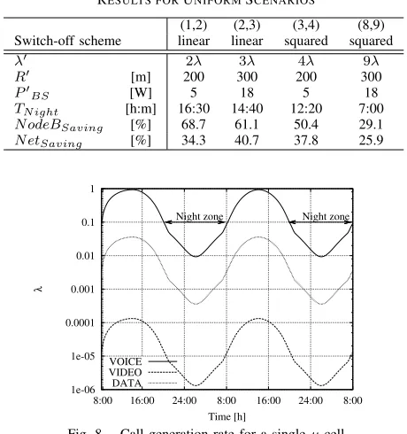
For the same uniform scenario, with a large number of identical microcells arranged in a grid, we can look at different switch-off patterns, wherekout ofN Node-B’s are switched off during the night zone, assuming that the N cells are arranged in either a line or a square (recall that one Node-B corresponds to each cell) and that the Node-B is in the center of the cell. The considered schemes are reported in Fig. 2. On the top left there is the (k, N) = (1,2) linear scheme, where 1 Node-B is switched off for every 2 adjacent cells in the same row, as the case we just discussed (notice that results are different because we consider a different traffic pattern). The top right scheme is the (2,3) linear; the bottom left corresponds to (3,4) square, in this scheme 3 Node-B’s are switched off for each2×2square of cells and, finally, the (8,9) square case is represented by the bottom right scheme of the figure. We consider the call generation rate as in Fig. 8. Table IV reports the results. Observe that the individual Node-B power saving can be huge, higher than 60%, and the overall access network power saving can be larger than 40%. However, somewhat surprisingly, these huge gains are not achieved by turning off the largest fraction of Node-B’s, since this choice reduces the duration of the night zone because of the traffic increase at the Node-B’s that remain active. Thus, a very careful choice of the switch-off pattern, made possible by our approach, is essential to minimize the energy consumption.
B. Hierarchical scenario
TABLE IV
RESULTS FORUNIFORMSCENARIOS
(1,2) (2,3) (3,4) (8,9) Switch-off scheme linear linear squared squared
λ′ 2λ 3λ 4λ 9λ
R′ [m] 200 300 200 300
P′
BS [W] 5 18 5 18
TN ight [h:m] 16:30 14:40 12:20 7:00
N odeBSaving [%] 68.7 61.1 50.4 29.1
N etSaving [%] 34.3 40.7 37.8 25.9
1e-06 1e-05 0.0001 0.001 0.01 0.1 1
8:00 16:00 24:00 8:00 16:00 24:00 8:00
λ
Time [h]
Night zone Night zone
VOICE VIDEO DATA
Fig. 8. Call generation rate for a singleµ-cell
cover shadowed regions and fill gaps in coverage, or to manage overflow traffic. In our scenario, the transmitted power at the base station is PBS= 5W for eachµ-cell, and 10 W for the
umbrella cell. One Node-B controls the umbrella cell, and two Node-B’s control the 6 µ-cells, The call generation rate has the day/night pattern reported in Fig. 8. The ratio between the peak and the minimum call generation rates is about 100.
The switch-off scheme consists in switching off the 6 µ-cells during night, so as to turn off the Node-B’s that control them. The radius of the circular umbrella cell is about 245
m, computed from the total area covered by the six µ-cells. During night, the call generation rate at the umbrella cell is six times the one of the singleµ-cell. Fig. 9 shows the maximum radius, Rmax, versus the average power for a connection,
Pconn, as derived from the Link-Budget limits. The curves are
flat when the UL limits the maximum radius, i.e., when the tighter constraint is given by the mobile station transmission power; the curves are increasing when the radius is limited by the DL, as is usually the case for small cells in urban, dense, areas. In our case, with radius 245 m, the umbrella cell needs a minimum Pconn= 17.32dBm, that corresponds to a
transmission powerPBS of about 9 W.
From the results we see that the 6 µ-cells covered by the umbrella cell can be switched off for about 10.5 hours (in the period from 20:45 to 07:15), while, in order to guarantee continuous coverage, the umbrella cell is always on. Since 2 Node-B’s out of 3 can be switched off, the overall possible power saving is almost 30%.
Also in this case, this power saving is achievable if Node-B’s are switched off as soon as the traffic level and the transmission parameters allow it. This is possible with forced handovers. Waiting for all services in progress at the time
50 100 150 200 250 300 350 400 450 500 550 600
5 10 15 20 25 30 35
Rmax
[m]
Ptxconn [dbm] VOICE
VIDEO DATA
Fig. 9. Maximum radius variation versus average power per connection (Hierarchical scenario - umbrella cell)
of the switch-off decision to terminate, but admitting no new call, the saving is reduced. In Fig. 7, the curve labeled
hierarchical shows the distribution of the time required to reach the idle state for Node-B’s. We can see that the cell is emptied with 90%probability after about 15 minutes. This implies a marginal reduction in power saving.
VI. CONCLUSIONS
We presented a novel approach for the energy-aware man-agement of UMTS access networks, that, based on the instan-taneous traffic intensity, reduces the number of active access devices when they are underutilized.
Numerical results indicate that the fraction of energy saved by implementing the proposed schemes can be huge, provided that the switch-off periods, and the Node-B’s to be switched off, are carefully chosen, as made possible by our approach.
REFERENCES
[1] Global Action Plan, An inefficient truth, http://www.globalactionplan.org.uk/, Report, 2007.
[2] S. Pileri, Energy and communication: engine of the human progress, http://www.ega.it/intelec2007/img/Stefano Pileri.pdf, Intelec Opening Keynote Speech, 2007.
[3] L. Chiaraviglio, D. Ciullo, M. Meo, M. Ajmone Marsan,Energy-Aware UMTS Access Networks, W-GREEN 2008, Lapland.
[4] J.T. Louhi,Energy efficiency of modern cellular base stations, INTELEC 2007, Rome, Italy.
[5] Vodafone using Ericssons new power-saving base station feature, http://www.3g.co.uk/PR/Dec2007/5524.htm, 2007.
[6] M. Hodes,Energy and power conversion: A telecommunication hardware vendors perspective, http://www.peig.ie/pdfs/ALCATE˜1.PPT, Power Electronics Industry Group, 2007.
[7] Node B datasheets, http://www.motorola.com/, 2008.
[8] J. Lempiinen, M. Manninen, Radio Interface System Planning for GSM/GPRS/UMTS, Kluwer Academic Publ., Hingham, MA, USA, 2001. [9] Cost 231 Final Report, http://www.lx.it.pt/cost231/.
[10] A. Boukerche,Handbook on Algorithms for Wireless Networking and Mobile Computing, Chapman and Hall CRC, New York, USA, 2005. [11] J. Ferreira, F. Velez, E. M. Reguera, Classification of mobile
multimedia services, Seacorn Project Public Deliverables, 2002, http://seacorn.ptinovacao.pt/docs/public deliverables/D PTIN WP1 11b8.zip. [12] J. Ferreira, A. Gomes and F.J.Velez,Enhanced UMTS Deployment and
Mobility Scenarios,in Proc. of 12th IST Mobile & Wireless Communi-cations Summit, Aveiro, Portugal, June 2003.