CSUSB ScholarWorks
CSUSB ScholarWorks
Electronic Theses, Projects, and Dissertations Office of Graduate Studies
12-2017
An Introduction to Lie Algebra
An Introduction to Lie Algebra
Amanda Renee Talley
California State University – San Bernardino
Follow this and additional works at: https://scholarworks.lib.csusb.edu/etd
Part of the Algebra Commons
Recommended Citation Recommended Citation
Talley, Amanda Renee, "An Introduction to Lie Algebra" (2017). Electronic Theses, Projects, and Dissertations. 591.
https://scholarworks.lib.csusb.edu/etd/591
A Thesis
Presented to the
Faculty of
California State University,
San Bernardino
In Partial Fulfillment
of the Requirements for the Degree
Master of Arts
in
Mathematics
by
Amanda Renee Talley
A Thesis
Presented to the
Faculty of
California State University,
San Bernardino
by
Amanda Renee Talley
December 2017
Approved by:
Dr. Giovanna Llosent, Committee Chair Date
Dr. Gary Griffing, Committee Member
Dr. Hajrudin Fejzic, Committee Member
Dr. Charles Stanton, Chair, Dr. Corey Dunn
Department of Mathematics Graduate Coordinator,
Abstract
An (associative) algebra is a vector space over a field equipped with an
associa-tive, bilinear multiplication. By use of a new bilinear operation, any associative algebra
morphs into a nonassociative abstract Lie algebra, where the new product in terms of the
given associative product, is the commutator. The crux of this paper is to investigate the
commutator as it pertains to the general linear group and its subalgebras. This forces
us to examine properties of ring theory under the lens of linear algebra, as we determine
subalgebras, ideals, and solvability as decomposed into an extension of abelian ideals, and
nilpotency, as decomposed into the lower central series and eventual zero subspace. The
map sending the Lie algebra L to a derivation of L is called the adjoint representation,
where a given Lie algebra is nilpotent if and only if the adjoint is nilpotent. Our goal is
to prove Engel’s Theorem, which states that if all elements of Lare ad-nilpotent, thenL
Acknowledgements
I would like to thank the members of my Graduate Committee: Dr. Giovanna
Llosent, Dr. Gary Griffing, and Dr. Hajrudin Fejzic for their invaluable guidance and
patience in helping me construct and review this document. I would also like to thank
my husband, Andrew Wood, for his continued resilience and support throughout this
Table of Contents
Abstract iii
Acknowledgements iv
List of Figures vi
1 Introduction 1
2 Definitions and First Examples 11
2.1 The Notion of a Lie Algebra and Linear Lie Algebras . . . 11
2.2 Classical Lie Algebras . . . 13
2.3 Lie Algebras of Derivations . . . 17
2.4 Abstract Lie Algebras . . . 19
3 Ideals and Homomorphisms 23 3.1 Ideals . . . 23
3.2 Homomorphisms and Representations . . . 29
3.3 Automorphisms . . . 37
4 Solvable and Nilpotent Lie Algebras 42 4.1 Solvability . . . 42
4.2 Nilpotency . . . 45
4.3 Proof of Engel’s Theorem . . . 49
5 Conclusion 53
List of Figures
3.1 Table of eigenvalues . . . 27
3.2 Table of eigenvalues forB2 . . . 34
3.3 Table of eigenvalues forC2. . . 35
Chapter 1
Introduction
Abstract Lie algebras are algebraic structures used in the study of Lie groups.
They are vector space endomorphisms of linear transformations that have a new operation
that is neither commutative nor associative, but referred to as the bracket operation, or
commutator. Recall that an associative algebra preserves bilinear multiplication between
elements in a vector spaceV over a fieldF, whereV×V →V is defined by (x, y)→xyfor x, y ∈V. The bracket operation yields a new bilinear map, over the same vector space, that turns any associative algebra into a Lie Algebra, where V ×V →V is now defined by [x, y] → (xy −yx). Central to the study of Lie algebras are the classical algebras, which will be explored throughout this paper to derive isomorphisms, identify simple
algebras, and determine solvability. After examining some natural Lie algebra examples,
we will delve into the derived algebra, which is analogous to the commutator subgroup of
a group, and make use of it to define a sequence of ideals called the derived series, which
is solvable. We will then use a different sequence of ideals called the descending central
series to classify nilpotent algebras. All of this will arm us with the necessary tools to
prove Engel’s Theorem, which states that if all elements ofL are ad-nilpotent, then Lis
nilpotent. We must first recall some basic group axioms, ring axioms, and vector space
The study of Lie Algebra requires a thorough understanding of linear algebra,
group, and ring theory. The following provides a cursory review of these subjects as
they will appear within the scope of this paper. Unless otherwise stated, our refresher
for group theory was derived from Aigli Papantonopoulou’s text Algebra Pure and
Applied [Aig02].
Definition 1.1. An associative algebra is an algebraAwhose associative rule is
associa-tive: x(yz) = (xy)z for all x, y, z∈A
Definition 1.2. A nonempty set G equipped with an operation ∗ on it is said to form a group under that operation if the operation obeys the following laws, called the group
axioms:
• Closure: For any a, b∈G, we havea∗b∈G.
• Associativity: For any a, b, c∈G, we have a∗(b∗c) = (a∗b)∗c.
• Identity: There exists an element e ∈G such that for all a∈G we have a∗e= e∗a=a. Such an element e∈G is called an identity in G.
• Inverse: For each a ∈ G there exists an element a−1 ∈ G such that a∗a−1 = a−1∗a=e. Such an element a−1 ∈G is called an inverse of a in G.
Proposition 1.3. (Basic group properties) For any group G
• The identity element of G is unique.
• For each a∈G, the inverse a−1 is unique.
• For any a∈G, (a−1)−1=a
• For any a, b∈G, (ab)−1 =b−1a−1
• For any a, b ∈ G, the equations ax = b and ya = b have unique solutions or, in other words, the left and right cancellation laws hold.
Example 1.0.1. Thegeneral linear group, denotedgl(n), consists of the set of
invert-ible n×n matrices. By the above, given that multiplication of invertible n×n matrices is associative, and each invertible matrix has an inverse and an identity, gl(n) forms a
Definition 1.4. nonempty subset H of a group G is a subgroup of G if H is a group
under the same operation as G. We use the notation H⊂Gto mean that H is a subset of G, andH ≤Gto mean thatHis a subgroup ofG. For a groupGwith identity element
e, {e} is a subgroup of G called the trivial subgroup. For any group G, G itself is a subgroup of G, called the improper subgroup. Any other subgroup of Gbesides the two
above is called a nontrivial proper subgroup of G.
Definition 1.5. The number of elements in a group G is called the order of G and is
denoted |G|. G is a finite group if |G| is finite. If a ∈ G, the order |a| of a in G is the least positive integer nsuch that an=e. If there exists no such integer n, then |a|is infinite.
Definition 1.6. A map ϕ : G → G0 from a group G to a group G0 is called a homo-morphism if ϕ(ab) = ϕ(a)ϕ(b) for all a, b∈ G (in ϕ(ab) the product is being taken in
G, while in ϕ(a)ϕ(b) the product is being taken in G0).
Proposition 1.7. (Basic group homomorphism properties) Let ϕ :G → G0 be a homomorphism. Then
• ϕ(e) =e0, where e is the identity ofG and e0 the identity of G0.
• ϕ(a−1) = (ϕ(a))−1 for anya∈G
• ϕ(an) =ϕ(a)n for any n∈Z
• If |a|is finite, then |ϕ(a)|divides |a|.
• If H is a subgroup of G, then ϕ(H) ={ϕ(x)|x∈H} is a subgroup of G0
• If K is a subgroup of G0, then ϕ−1(K) ={x∈G|ϕ(x)∈K} is a subgroup of G.
Example 1.0.2. For any group G, the identity map is always a homomorphism, since
if ϕ:G→G0 is the identityϕ(x) =x, then ϕ(xy) =xy=ϕ(x)ϕ(y)
Definition 1.8. For the homomorhpismϕ, thekernelofϕis the set{x∈G|ϕ(x) =e0}, denoted Ker ϕ.
Definition 1.9. Let G be a group, H a subgroup of G, and a∈G. Then the set aH =
Definition 1.10. The group consisting of the cosets of H in G under the operation
(aH)(bH) = (ab)H is called the quotient group of G by H, written G/H.
Definition 1.11. If Gis any group, then thecenter ofG, denoted Z(G), consists of the
elements of G that commute with every element ofG. In other words,
Z(G) ={x∈G|xy =yx ∀y∈G} (1.1)
Note that ey=y=yefor all y∈G, so e∈Z(G), and the center is a nonempty subset of
G. Let a∈G. Then the centralizer of ain G, denoted CG(a), is the set of all elements
of Gthat commute with a. In other words
CG(a) ={y∈G|ay=ya} (1.2)
Note that for any a∈G we have Z(G)⊆CG(a). In other words, the center is contained
in the centralizer of any element [Aig02].
Definition 1.12. Let G be a group and H a subgroup of G. If for all g ∈ G we have
gH =Hg, then we sayH is anormalsubgroup ofGand writeH /G. (Recall the normal
subgroup test: A subgroup H of G is normal in Gif and only if xHx−1⊆H for all x in
G) .
The following material for group and ring theory was derived from Joseph A.
Gallian’s Contemporary Abstract Algebra[Gal04].
Definition 1.13. An isomorphism from a group G onto itself is called an
automor-phism of G.
Definition 1.14. Let G be a group, and leta∈G. The function ϕa defined by ϕa(x) =
axa−1 for allx∈G is called theinner automorphism of G induced by a.
Definition 1.15. A set R equipped with two operations, written as addition and
multi-plication, is said to be a ring if the following four ring axioms are satisfied, for any
elements, a, b, and c in R:
• R is an Abelian group under addition.
• Associativity: a(bc) = (ab)c.
• Distributivity: a(b+c) =ab+ac and (b+c)a=ba+ca.
Definition 1.16. A subring A of a ringR is called a (two-sided) idealof R if for every
r ∈R and every a∈A both ra andar are in A.
Theorem 1.17. Ideals are Kernels Every ideal of a ring R is the kernel of a ring
homomorphism of R. In particular, an ideal A is the kernel of the mapping r → r+A
from R to R/A.
Definition 1.18. Aunity(or identity) in a ring is a nonzero element that is an identity
under multiplication. A nonzero element of a commutative ring with unity that has a
multiplicative inverse is called a unit of the ring.
Theorem 1.19. First Isomorphism Theorem for RingsLet ϕbe a ring
homomor-phism from R→S. Then the mapping from R/kerϕ to ϕ(r), given by r+kerϕ→ϕ(r) is an isomorphism. In symbols, R/kerϕ∼=ϕ(r)
Theorem 1.20. Second Isomorphism Theorem for Rings If A is a subring of R
andB an ideal ofR, thenA∩B is an ideal ofAandA/A∩B is isomorphic to(A+B)/B. (Recall that {A+B =a+b|a∈A, b∈B})
Theorem 1.21. Third Isomorphism Theorem for Rings Let A and B be ideals of
a ring R withB ⊆A. A/B is an ideal of R/B and (R/B)(A/B) is isomorphic to R/A.
Theorem 1.22. Correspondence TheoremLetI be an ideal of a ringR. There exists
a bijection between the set of all ideals J ofR such thatI ⊂J and the set of all ideals of
R/I:
{J|I is an ideal of R, I ⊂J} → {K|K is an ideal of r/I}
J →J/I
Definition 1.23. In a ring R the characteristic of R, denoted char R, is the least
positive integer n such that n·a = 0 for all a ∈ R. If no such n exists, we say char
R= 0.
Definition 1.24. A field is a commutative ring with unity in which every nonzero
Unless otherwise stated, the material for our vector space review was derived
from Stephen H. Friedberg et al’s,Linear Alebra [FIS03].
Definition 1.25. Let F be a field. A set V equipped with two operations, written as
addition and multiplication, is said to be a vector space over F if
• V is an Abelian group under addition. For all a, b∈F and all u, v∈V,
• The product av∈V is defined
• a(v+w) =av+aw
• a(bv) = (ab)v
• 1v =v
An element of v ∈ V is called a vector. The identity element of V under addition is called the zero vector and written 0. An element of a∈ F is called a scalar, and the operation of forming av is calledscalar multiplication [Aig02].
Definition 1.26. A subset U of a vector space V over a fieldF is called asubspace of
V if U is a vector space over F with the operations of addition and scalar multiplication
defined on V
Example 1.0.3. IfT :V →W is a linear map, thekernelofT and theimage (range) of T defined by
ker(T) ={x∈W :T(x) = 0}
im(T) ={w∈W :T(x), x∈W}
are subspaces of V.
Definition 1.27. Let V be a vector space over a field F. A vector space homomorphism
that maps V to itself is called an endomorphism of V
Definition 1.28. Let V andW be vector spaces. We say thatV isisomorphictoW if
Definition 1.29. LetV be a vector space over C. Aninner product onV is a function
that assigns, to every ordered pair of vectors x and y in V, a scalar inC, denotedhx, yi, such that for all x, y, z in V and all c in C, the following hold:
1. hx+z, yi=hx, yi+hz, yi
2. hcx, yi=chx, yi
3. hx, yi=hy, xi
4. hx, xi>0 if x6= 0
Definition 1.30. Let V be a vector space over a fieldF. A functionf from the setV×V
of ordered pairs of vectors to F is called a bilinear form on V if f is linear in each
variable when the other variable is held fixed; that is, f is a bilinear form onV if
1. f(αx1+x2, y) =αf(x1, y) +f(x2, y)
2. f(x, αy1+y2) =αf(x, y1) +f(x, y2)
Any nondegenerate bilinear form on V consists of all operators x on V
un-der which the form f is infinitesimally invariant, i.e., that satisfies f(x(v), w) +
f(v, x(w)) = 0. [FIS03]
The kernel of a symmetric bilinear form is given as: kerf ={v:f(v, w) = 0 for all w∈V}. That is, for all v∈W, there exists a w∈V such thatf(v, w) = 0.
Definition 1.31. Analternating spaceis defined as the set of all vector spaces V and
alternate bilinear forms such that f :V ×V →F where: 1. f(x, y+z) =f(x, y) +f(x, z)
2. f(x+y, z) =f(x, z) +f(y, z)
3. f(ax, y) =af(x, y) =f(x, ay)
4. f(x, x) = 0 which implies that f(x, y)=-f(y,x)
Definition 1.32. In matrix terms, an n-linear function γ : Mn×n(F) → F is called
alternating if, for each A ∈ Mn×n(F), we have γ(A) = 0 whenever two adjacent rows
Theorem 1.33. Let A be an m×nmatrix,B and C be n×p matrices andD andE be
q×m matrices. Then
1. A(B+C) =AB+AC and (D+E)A=DA+EA
2. α(AB) = (αA)B = (AαB)
3. ImA=A=AIm
4. IfV is an n-dimensional vector space with an ordered basis B, then [IV]B=In
Definition 1.34. Let A, B and C be matrices where C = cij, A = ajk, and B = bkj.
Then by matrix multiplication
C=AB where cij = n
X
k=1
aikbkj
The formula for the determinant of A, denoted det(A) or |A|, where A is a n×n
matrix can be expressed as cofactor expansion along the 1st row of A
det(A) =
n
X
j=1
(−1)i+jAij·det( ˜Aij)
Where the scalar cij = (−1)i+jdet( ˜Aij) is called the cofactor of the entry ofA if row i,
column j.
Example 1.0.4. The Laplace expansion of A where A is a 2×2 matrix is
det(A) =A11(−1)1+1detA˜11+A12(−1)1+2detA˜12
Definition 1.35. (Adjoint of a Matrix) LetA be an n×nmatrix. The matrix B = [bij]
withbij =cji (forcij as defined in Definition 1.33), for1≤i, j≤nis called theAdjoint
of A,denoted Adj(A).
Definition 1.36. The traceof a matrix is the sum of its diagonal entries.
Definition 1.37. Given an n×n matrix A ={aij}, the transpose of A is the matrix
AT ={b
ij}, where bij =aji.
Definition 1.38. If the transpose of a matrix is equal to the negative of itself, the matrix
is said to be skew symmetric. This means that for a matrix to be skew symmetric,
Definition 1.39. Let F be a field and V, W vector spaces over the field F. A function
T :V →W is said to be alinear transformation from V to W if for all c, d∈F, and all x, y∈V we have
T(cx+yd) =cT(x) +dT(y)
The following are simple properties of linear transformations:
• T(0) = 0
• T(cx+y) =cT(x) +T(y)
• T(x−y) =T(x)−T(y)
• For x1, x2, ..., xn∈V and a1, a2, ..., an∈F, we have
T(
n
X
i=1
aixi) = n
X
i=1
aiT(xi)
Example 1.0.5. Consider the map T :Mn×n(F) → Mn×m(F) defined by T(A) = At.
We can show that T is a linear transformation. LetA=Aij and B =Bij
(A+B)t= (Aij +Bij)t= (Aij)t+ (Bij)t=At+Bt
T(cAij) = (cAij)t=c(Aij)t=cAt
Definition 1.40. A basis, β, for a vector space V is a linearly independent subset ofV
that generates V. If there exists a finite set that forms a basis forV over a field F, then
the number n of vectors in such a basis {v1...vn} is called the dimension of V over F,
written dim FV. If there exists no finite basis forV overF, thenV is said to beinfinite
dimensional over F.
Definition 1.41. Let T =TA :V →V be a linear transformation, where V is a
finite-dimensional vector space over a field F, and let 0 6=v ∈V be such that TA(v) = λv for
some λ∈F. Then v is called aneigenvector of T (and ofA), and λ the corresponding eigenvalue of T (and of A).
Definition 1.43. a matrix M ∈Mn×n(F) is called orthogonal if M Mt=I.
Theorem 1.44. If A is a square matrix of order n > 1, then A(adjA) = (adjA)A =
|A|In. The (i, j)th element ofA(adjA) is: n
X
k=1
aikakj = n
X
k=1
aijAjk =
|A| ⇔i=j 0⇔i6=j
Therefore A(adjA) is a scalar matrix with diagonal elements all equal to |A|.
⇒A(AdjA) =I(n)
⇒(AdjA)A=|A|I(n) Where |A|represents the determinant of A.[Eve66]
Proposition 1.45. The following equation denotes the inverse of A:
A−1= AdjA
|A|
Definition 1.46. If A is a square matrix of order n, then the λ matrix [A −λI(n)] is called the characteristic matrix of A. The determinant |A−λI(n)| is called the characteristic determinant of A, and the expansion of it is a polynomial of degreen:
f(λ) = (−1)n[λn−p1λn−1+p2λn−2+...(−1)npn]
[Eve66]
Chapter 2
Definitions and First Examples
2.1
The Notion of a Lie Algebra and Linear Lie Algebras
Let R be a fixed commutative ring (or a field). An associative R-algebra is
a group A that is abelian under addition, and has the structure of both a ring and
an R-module such that the scalar multiplication satisfies r ·(xy) = (r·x)y = x(r·y) for all r ∈ R and x, y ∈ A. Additionally, A contains a unique element 1 such that 1·x = x = x·1 for all x ∈ A. A is therefore an R-module together with (1) an R -bilinear map A×A → A, called the product, and (2) the multiplicative identity, such that multiplication is associative: x(yz) = (xy)z, for allx, y, andz inA. If one negates
the requirement for associativity, then one obtains a non-associative algebra. IfAitself is
commutative, it is called a commutative R-algebra. The commutator of two elements x
andyof a ring or an associative algebra is defined byxy−yx. (The anticommutator of two elements x and y of a ring or an associative algebra is defined by{x, y}=xy+yx). Any algebraA overF, whereF is a vector space with associative multiplication can be made
into a Lie algebra L via the commutator, yielding a structure similar to a ring modulo
L. The commutator is also referred to as the the bracket operation. In order to prove
Engel’s Theorem, we shall restrict ourselves to the following definition of abstract Lie
algebra, in contrast to the concrete Lie algebra definition featured in universal enveloping
algebras and the Poincare Birkhoff Witt Theorem. Additionally, we will assume all base
Definition 2.1. A vector spaceL over a fieldF, is a Lie algebra if there exists a bilinear
multiplication L×L→L, with an operation, denoted(x, y)7→[xy], such that: 1. It isskew symmetric where [x, x] = 0for all x in L (this is equivalent to
[x, y] =−[y, x]since character F 6= 2).
2. It satisfies the Jacobi identity[x[yz]] + [y[zx]] + [z[xy]] = 0 (x, y, z∈L).
Example 2.1.1. Given an ndimensional vector space End (V), the set of all all linear
maps V 7→ V with associative multiplication (x, y) 7→ xy for all x, y, where xy denotes functional composition, observe, End (V) is an associative algebra over F. Let us define
a new operation on End (V) by (x, y) 7→ xy−yx. If we denote xy−yx by [x, y], then End (V) together with the map[·,·] satisfies Definition 2.1, and is thus a Lie algebra. Proof. The first two bracket axioms are satisfied immediately. The only thing left to
prove is the Jacobi identity. Given x, y, z ∈ End (V), we have by use of the bracket operation:
[x[yz]] + [y[zx]] + [z[xy]] = 0
=x(yz−zy)−(yz−zy)x+y(zx−xz)−(zx−xz)y+z(xy−yx)−(xy−yx)z =xyz−xzy−yzx+zyx+yzx−yxz−zxy+xzy+zxy−zyx−xyz+yxz = (xyz−xyz) + (xzy−xzy) + (yzx−yzx) + (zyx−zyx) + (yxz−yxz) = 0
Definition 2.2. The Lie algebra End (V) with bracket [x, y] =xy −yx, is denoted as
gl(V), the general linear algebra.
Example 2.1.2. We can show that real vector space R3 is a Lie algebra. Recall the
following cross product properties when a, b and c represent arbitrary vectors and α, β
and γ represent arbitrary scalars:
1. a×b=−(b×a),
([MT03])
Note, a×a=−(a×a), by property (1), letting b=a, therefore,a×a= 0. By the above properties, the cross product is both skew symmetric (property 1) and bilinear (property
2). By vector triple product expansion: x×(y×z) =y(x·z)−z(x·y). To show that the cross product satisfies the Jacobi identity, we have:
[x[y, z]] + [y[z, x]] + [z[x, y]] =x×(y×z) +y×(z×x) +z×(x×y)
= [y(x·z)−z(x·y)] + [z(y·x)−x(y·z)] + [x(z·y)−y(z·x)] = 0 {Since the dot product is commutative}
Therefore, by definition 2.1, the real vector space R3 is a Lie algebra
Definition 2.3. A subspace K of L is called a (Lie) subalgebra if [xy]∈K whenever
x, y∈K.
2.2
Classical Lie Algebras
Classical algebras are finite-dimensional Lie algebras. Each classical algebraAl,
Bl,Cl, andDlhas an associated algebra, represented by symmetric, skew symmetric, and
orthogonal matrices. Letsbe ann×nmatrix. We shall prove that each classical algebra representation, equipped with basis and dimension satisfyingxs+sxt= 0 (xt=transpose ofx), is a subalgebra of the linear Lie algebragl(V). Note: a proper subalgebra maintains
dimension less than that of gl(n).
(Al) The set of all endomorphisms ofV having trace zero is denoted bysl(V), the
special linear algebra. Lettingx, y∈sl(V), we can show that sl(V) is a subalgebra of
gl(V).
Proof.
tr[x, y] =tr(xy)−tr(yx) = 0 {Since the trace of a matrix preserves bilinearity}
tr([x,[y, z]] + [y,[z, x]] + [z,[x, y]]) =tr[x,0] +tr[y,0] +tr[z,0] = 0
Therefore, both Lie algebra axioms are satisfied, hence by Definition 2.3, sl(V) is a
The dimension of sl(V) is found by determining the number of linearly independent
matrices of sl(V) that yield trace 0. By counting the matriceseij(i6=j), and adding
them to the matrices hi =eij−ei+1,i+1, we find dimsl(V) =l+ (l+ 1)2−(l+ 1) (Cl) The set of endomorphisms of V having dimV = 2l, that satisfies
f(v, w) =−f(w, v), is denoted as sp(V), the symplectic algebra. Let sbe a nondegenerate, skew symmetric matrix where s=
0 Il
−Il 0
. Recall that a matrix
A∈Mn×n(F) is calledskew-symmetric ifAt=−A. We can showsp(2l, F) is a
subalgebra of gl(V) if we partitionx asx=
m n
p q
wherem, n, p, q∈gl(v).
Proof. Givenx, y∈sp(V), f([xy](v), w) +f(v,[xy](w))
=f((xy−yx)v, w) +f(v,(xy−yx)w) {By definition of the bracket operation}
=f(xy(v), w)−f(yx(v), w) +f(v, xy(w))−f(v, yx(w)) {By definition of bilinearity}
=f(x(y(v)), w)−f(y(x(v)), w) +f(v, x(y(w))−f(v,(y(x(w))
=−f(y(v), x(w)) +f(x(v), y(w))−f(x(v), y(w)) +f(y(v), x(w)) {By skew symmetry}
=0
Therefore [x, y]∈sp(V), hence sp(V) is a subalgebra ofgl(V) whensp(v) is of even dimension. We show that sp(V) requires even dimensionality by considering the
determinant of x when nis odd. Fromsx=−xts,
det(sx) =det(−xts) ⇐⇒ det(s)det(x) =det(−xt)det(s)
⇐⇒ det(x) =det(−xt) = (−1)ndet(xt) = (−1)2k−1det(xt) =−det(xt)
but then det(x) =−det(xt), therefore, det(x) = 0
(Bl) The set of all endomorphisms of V with dimension 2l2+l satisfying
matrix s=
1 0 0
0 0 Il
0 Il 0
, corresponds to theorthogonal algebra, denoted as o(V), or
o(2l+ 1, F). Recall a matrix A∈Mn×n(F) is called orthogonalifAAt=I. We can
partition xas x=
a b1 b2
c1 m n
c2 p q
. The orthogonal algebra is a subalgebra ofgl(V),
where f(x(v), w) =−f(v, x(w)) (the same conditions as for (Cl).
Example 2.2.1. When V =Fn, take for f(x(v), y) the formP
XiY =xty where
X = (x1, x2, ..., xn) and Y = (y1, y2, ..., yn). The corresponding Lie algebra is o(n, F)
(Dl) LetDl be an an orthogonal algebra withs=
0 Il
Il 0
. Letm= 2l, thenDl
consists of all the matrices with dimension 2l2−l, satisfying f(x(v), w) =−f(v, x(w)).
Definition 2.4. The following is a list of several other subalgebras consisting of the
upper, lower, and triangular matrices of gl(n, F):
• Let n(n, F) be the strictly upper triangular matrices (aij) = 0 if i≥j
• Let d(n, F) be the set of all diagonal matrices (aij), aij = 0 if i6=j.
• Let t(n, F) be the set of upper triangular matrices (aij), aij = 0 if i > j.
Example 2.2.2. Given algebras t(n, F),o(n, F),n(n, F), we can compute the dimension
of each algebra, by exhibiting a basis.
• For n(n, F) =
0 a12 ... a1n
0 0 ... a2n
..
. ... . ..
0 0 · · · 0
• For o(n, F) =
a11 0 ... 0
0 a22 ... 0
..
. ... . ..
0 0 · · · ann
The dimension of o(n, F) is clearly n.
• For t(n, F)=
a11+ a12 ... a1n
0 a22 ... a2n
..
. ... . ..
0 0 ... ann
Again using the formula for the area of a triangle, the dimension of t(n, F) is
n(n+1) 2
Definition 2.5. The (external)direct sum of two Lie algebras L, L0, written L⊕L0 is the vector space direct sum, with [·,·]defined “componentwise”: [(x1, y1),(x2, y2)] where
{(x,0)},{(y,0)} are ideals and thus ”nullify” each other. That is, [L, L0] = 0. [Sam90]
Example 2.2.3. We can prove that t(n, F) is the direct sum ofo(n, F) and n(n, F). By
the above definition, we must show [t(n, F),t(n, F)] = 0 where
t(n, F) =o(n, F) +n(n, F).
Proof. LetA∈n(n, F) and B ∈o(n, F), andC ∈t(n, F):
0 a12 ... a1n
0 0 ... a2n
..
. ... . ..
0 0 · · · 0
+
b11 0 ... 0
0 b22 ... 0
..
. ... . ..
0 0 · · · bnn
=
b11 a12 ... a1n
0 b22 ... a2n
..
. ... . ..
0 0 ... bnn
where A+B is an upper diagonal matrix. Thereforet(n, F) =o(n, F) +n(n, F). To
show A∩B ={0}, we have
(AB)ij = i
X
k=1
AikBkj + n
X
k=i+1
AikBkj
=
i
X
k=1
0·Bkj+ n
X
k=i+1
Aik·0
Where Aik = 0 in the first sum sincei≥kforA strictly upper triangular. For the
AB−BA= [AB] = 0. Therefore [o(n, F),n(n, F)]⊆n(n, F). We can construct a basis eij forn(n, F) such thateij is 1 for the (ij) element, and zero elsewhere. By definition
of the commutator:
[eii, eij] =eiieij −eijeii=eij
By the above, when i≥j,n(n, F)⊆[o(n, F),n(n, F)], and thus [o(n, F),n(n, F)] =n(n, F). Since o(n, F) +n(n, F) =t(n, F):
[o(n, F) +n(n, F),o(n, F) +n(n, F)] = [o(n, F),o(n, F)] + [n(n, F),n(n, F)]
[n(n, F),o(n, F)] + [o(n, F),n(n, F)]
= 0 + 0 + [o(n, F),n(n, F)]⊆n(n, F) Conversely:
n(n, F) = [o(n, F),n(n, F)]⊆[t(n, F),t(n, F)] Therefore [t(n, F),t(n, F)] =n(n, F) and thust(n, F) =o(n, F) +n(n, F)
2.3
Lie Algebras of Derivations
The derivative between two functions f and g is a linear operator that satisfies the
Leibniz rule:
1. (f g)0 =f0g+f g0
2. (αf)0 =αf0 where α is a scalar.
Given an algebra A over a fieldF, the derivation ofA is the linear mapδ such that
δ(f, g) =f δ(g) +δ(f)gfor all f, g∈A. The set of all derivations ofA is denoted by Der(A). Given δ∈Der(A),f, g∈A, and α∈F. By property 2.,
(αδ)(f g) =αδ(f g) =α(f δ(g) +δ(f)g) =αf δ(g) +αδ(f)g
where the Leibniz rule is satisfied if and only if af =f awhere F is a field.
• Der(V) is a vector subspace of End(V):
δ[x, y] =δ(xy−yx) =δ(xy)−δ(yx) =xδ(y) +δ(x)y−(yδ(x) +δ(y)x) =δ(y)x−yδ(x) +xδ(y)−δ(y)x = [δ(x), y] + [x, δ(y)]
• The commutator [δ, δ0]of two derivations δ, δ0 ∈Der(V) is again a derivation. ([δ, δ0](x))y+x([δ, δ0](y)) = ((δδ0−δ0δ)(x))y+x(δδ0−δ0δ)(y)
= (δδ0(x)−δ0δ(x))y+x(δδ0(y)−δ0δ(y)) =δδ0(x)y−δ0δ(x)y+xδδ0(y)−xδ0δ(y) =δ(δ0(x)y+xδ0(y))−δ0(δ(x)y+xδ(y)) =δ(δ0(x)y) +δ0(x)δ(y) +δ(x)δ0(y) +xδ(δ0(y))
−δ0(δ(x)y)−δ(x)δ0(y)−δ0(x)δ(y)−xδ0δ(y) =δ(δ0(x)y+xδ0(y))−δ0(δ(x)y+xδ(y)) =δ(δ0(xy))−δ0(δ(xy))
= [δ, δ0](xy)
Definition 2.6. Given x∈L, the map y→[x, y], is an endomorphism of L, denoted adx, whereadx is an inner derivation. Derivations of the form[x[yz]] = [[xy]z] + [y[xz]]
are inner. All others are outer.
Example 2.3.2. By example 2.3.1, the collection of derivations, Der(V), satisfies skew
symmetry. By definition 2.6, Der(V) satisfies the Jacobi identity. Therefore Der(V)
defines a Lie algebra.
Definition 2.7. The mapL→DerLsending x to adx is called the adjoint
representation of L.
This is akin to taking the ad homomorphism of g→gl(g). To show ad is a homomorphism:
if and only if:
[[x, y], z] = [x,[y, z]]−[y,[x, z]]
0 = [x,[y, z]] + [y,[z, x]] + [z,[x, y]]
That is, if and only if the Jacobi identity is satisfied, where [[x, y], z] =−[z,[x, y]] and
−[y,[x, z]] = [y,[z, x]] by skew symmetry.
Definition 2.8. A representation is faithful if its kernal is zero, i.e., if
φ(x) = 0⇔x= 0, where the adjoint operator defines the trivial representation. [Sam90]
2.4
Abstract Lie Algebras
Let Lbe a finite dimensional vector space over F. Any vector space can be made into a
Lie algebra simply by setting [x, y] = 0 for all vectorsx and y inL. The resulting Lie
algebra is called abelian. Recall that a group Gunder multiplication is said to be
Abelian ifGobeys the commutativelaw or, that is, if for every a, b∈Gwe have ab=ba[Aig02]. If an associative algebra is abelian and therefore commutative, then
ab=ba⇔[a, b] = 0, where [a, b] is the associated commutator.
Example 2.4.1. Given L as a Lie algebra, with [xy] = 0for allx, y∈L, [xy] = (xy−yx) = 0⇔xy=yx
Therefore L under trivial Lie multiplication, is abelian. Similarly, [yx] = 0.
Definition 2.9. If L is any Lie algebra with basis x1, ..., xn, then the multiplication
table for L is determined by the structural constants, the set of scalars {bijk} such
that [xi, xj] =Pnk=1bijkxk.
Example 2.4.2. By use of the bracket axioms, the following set of structural constants
define an abstract Lie algebra:
1. biik = 0 =bijk+bjik
2. P
(bijkbklm+bjlkbklm+blikbkjm) = 0
1. Recall [xx] = 0 for all x∈L.
[xi, xi] = 0 = n
X
k=1
biikxk
=bii1x1+bii2x2+...+biinxn= 0.
Then, since xi is a basis,biik = 0 for all k.
2. Given [xi, xj] =Pnk=1bijkxk, noticebijk+bjik= 0 if and only if
X
k
(bijk+bjik)xk= 0 :
⇔X
k
bijkxk+
X
k
bjikxk= 0⇔[xixj] + [xjxi] = 0
But:
[xixj] =xixj−xjxi
[xjxi] =xjxi−xixj
⇔[xixj] + [xjxi] =xixj−xjxi+xjxi−xixj = 0
Definition 2.10. The assorted systems of structural constants of a given Lie algebra
relative to its basis form an orbit(the set of all transformations of one element) under
this action [Sam90].
Example 2.4.3. The orbit of the system cijk= 0 for alli, j, k forms a natural
isomorphism to the abelian algebra [X, Y] = 0 of dimensionn.
Example 2.4.4. Consider a Lie algebra L with basis x1, ...xn. The structural constants
are enumerated as followed: e1 = (1,0,0), e2= (0,1,0), and e3= (0,0,1). By use of the
Lie bracket axioms, We have:
[e1, e2] =e3
Therefore, by definition, the structural constants are:
b121 = 0, b122 = 0, b123 = 1,
b131 = 0, b132 =−1, b133= 0,
b231 = 1, b232 = 0, b233 = 0
Example 2.4.5. We can use structural constants to show that a three dimensional
vector space with basis (x, y, z) such that[xy] =z,[xz] =y,[yz] = 0defines a Lie
algebra.
Proof. the structural constants are:
b121 =b122= 0, b123= 1,
b131 =b133= 0, b132= 1,
b231 =b232=b233= 0
Where bijk=bijk−bjik = 0 for all structural constants above (by skew-symmetry). By
the Jacobi identity, we have:
[x[yz]] + [z[xy]] + [y[zx]] = [x,0] + [z, z] + [y.−y] = 0 + 0 + 0 = 0 Therefore the above basis defines a Lie algebra structure over F.
Definition 2.11. For any field F, in the vector space
Fn={(b1, b2, b3..., bn)|bi ∈F for 1≤i≤n}
a basis is formed by the vectors
e1 = (1,0, ...,0)
e2 = (0,1, ...,0)
.. .
en= (0,0, ...,1)
Where {e1, e2, ..., en} is called the standard basis for Fn over F.
Theorem 2.12. Let V and W be finite-dimensional vector spaces (over the same field).
Corollary 2.13. Let V be a vector space overF. Then V is isomorphic to Fn if and only if dim(V) =n[FIS03]
Chapter 3
Ideals and Homomorphisms
3.1
Ideals
Lie algebra ideals are intrinsic to much that follow. In group theory, ideals are used to
define the kernel of a group, normal subgroups, and the structure of nilpotent and
solvable groups. In a ring, every kernal is an ideal of a homomorphism, and every
subgroup is normal. By definition of the normal subgroup, if H is a subgroup of G, for
all g∈Gwe have gH =Hg⇔[g, H] = 0. Unless otherwise stated, the material for this chapter is derived from [Hum72].
Definition 3.1. A subspace I of a Lie algebra L is called an idealof L ifx∈I, y∈L
together imply [x, y]∈I. The construction of ideals in Lie algebra is analogous to the construction of normal subgroups in group theory.
By skew-symmetry, all Lie algebra ideals are automatically two sided. That is, if
[x, y]∈I, then [y, x]∈I. The kernel of a Lie algebra L andL itself are trivial ideals contained in every Lie algebra.
Example 3.1.1. The set of all inner derivations adx, x∈L, is an ideal of Der(L). Let
δ ∈ Der(L). By definition of inner derivations, for all y∈L: [δ, adx](y) = (δ(adx)−(adx)δ)(y) =δ[x, y]−adx(δ(y))
= [δ(x), y] + [x, δ(y)]−[x, δ(y)] {Since δ[x, y] = [δ(x), y] + [x, δ(y)]}
=ad(δ(x)y)
Definition 3.2. Thecenter of a Lie algebraL is the set
Z(L) ={z∈L|[x, z] = 0for all x∈L}
The center respresents the collection of elements in Lfor which the adjoint action ad(z) yeilds the zero derivation. It can therefore be thought of as the kernel of the adjoint
map fromL to Der(L). Clearly, the center is an ideal, thereforeZ(L) satisfies skew
symmetry. Given y∈L, [z,[x, y]] =−[x,[y, z]]−[y,[z, x]], both [y, z] and [z, x] belong toZ(L) by definition, therefore,Z(L) satisfies the Jacobi identity. IfZ(L) =L, thenL
is said to be albelian.
Definition 3.3. Thecentralizer of a subset X of L is defined to be
CL(X) ={x∈L|[x, X] = 0}
By the Jacobi, CL(L) is a subalgebra ofL whereCL(L) =ZL.
Definition 3.4. Consider the Lie algebra L, having two idealsI and J, the following
are ideals of L:
I+J ={x+y|x∈I, y∈J}
[I, J] =nXxiyi|xi ∈I, yi ∈J
o
Proposition 3.5. Let L be a Lie algebra and let I, J be subsets ofL. The subspace
spanned by elements of the form x+y (x∈I, y∈J), is denoted I+J, and the subspace spanned by elements of the form [x, y], (x∈I, y∈J), is denoted [I, J]. If I, I1, I2, J, K are subspaces of L, then
1. [I1+I2, J]⊆[I1, J] + [I2, J] 2. [I, J] = [J, I]
3. [I,[J, K]]⊆[J,[K, I]] + [K,[I, J]] [Wan75]
If I is an ideal of L, then the quotient spaceL/I (whose elements are the linear cosets
L+I) induces the well defined bracket operation, where [x+I, y+I] = [x, y] +I for
Definition 3.6. By use of the bracket operation [·,·], the quotient spaceL/I becomes a quotient Lie algebra [Sam90].
Definition 3.7. If the Lie algebraL has no ideals except itself and 0, and if moreover
[LL]6= 0, we call L simple.
Example 3.1.2. Let L be a Lie algebra, and L=sl(n,F) where char F 6= 2. It can be shown that L is simple if we take as a standard basis for L the three matrices
x= 0 1 0 0 , y =
0 0
1 0
, h=
1 0
0 −1
We will begin by computing the matrices of adx, adh, and ady.
• adx:
adx(x) = [x, x] = 0 = 0·x+ 0·h+ 0·y
adx(h) = [x, h] =xh−hx=
0 1 0 0 1 0
0 −1
−
1 0
0 −1
0 1 0 0 =
0 −1
0 0 − 0 1 0 0 =
0 −2
0 0
=−2x=−2·x+ 0·y+ 0·h
adx(y) = [x, y] =xy−yx=
0 1 0 0 0 0 1 0 − 0 0 1 0 0 1 0 0 = 1 0 0 0 − 0 0 0 1 = 1 0
0 −1
=h= 0·x+ 0·y+h
Therefore adx=
0 −2 0
0 0 1
0 0 0
• ady:
ady(x) = [y, x] =yx−xy=
0 0 1 0 0 1 0 0 − 0 1 0 0 0 0 1 0 = 0 0 0 1 − 1 0 0 0 =
−1 0
0 1
=−h
ady(y) = [y, y] = 0 = 0·x+ 0·h+ 0·y
ady(h) = [y, h] =yh−hy=
0 0 1 0 1 0
0 −1
−
1 0
0 −1
0 0 1 0 = 0 0 1 0 − 0 0
−1 0
= 0 0 2 0 = 2y
Therefore ady =
0 0 0
−1 0 0
0 0 2
• ad h:
adh(x) = [h, x] =hx−xh=
1 0
0 −1
0 1 0 0 − 0 1 0 0 1 0
0 −1
= 0 1 0 0 −
0 −1
0 0 = 0 2 0 0
= 2x= 2·x+ 0·h+ 0·y
adh(h) = [h, h] = 0 = 0·x+ 0·h+ 0·y
adh(y) = [h, y] =hy−yh=
1 0
0 −1
0 0 1 0 − 0 0 1 0 1 0
0 −1
= 0 0
−1 0
− 0 0 1 0 = 0 0
−2 0
=−2y= 0·x+ (−2)·y+ 0·h
Therefore adh=
2 0 0
0 0 0
0 0 −2
arbitrary. If adx is applied twice:
adx(ax+by+ch) =a[x, x] +b[x, y] +c[x, h] = 0 +bh−2cx
adx(0 +bh−2cx) =b[x, h]−2c[x, x] =−2bx
then −2bx∈I. If ad y is applied twice:
ady(ax+by+ch) =a[y, x] +b[y, y] +c[y, h] =−ah+ 0 + 2cy
ady(−ah+ 0 + 2cy) =−a[y, h] + 2c[y, y] =−2ay
then −2ay∈I. So if aor b is nonzero, than eithery or x is contained inI, thus I =L. If aand b are both zero, thench∈I where ch6= 0. Thus, again I =L. Therefore L is simple. [Hum72]
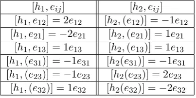
Example 3.1.3. We can show that sl(3, F) is simple, unless charF = 3, using the
standard basis h1, h2, eij(i6=j). If I6= 0 is an ideal, then I is the direct sum of
eigenspaces for ad h1 or adh2. We will determine the eigenvalues of by afixing h1 and
h2 toeij, i.e, take the adjoint using diagonal basis matrices. By definition of basis
matrices, for sl(3, F), h1=e11−e22 and h2=e22−e33. adh1(e12) = [h1, e12] =h1e12−e12h1
= (e11−e22)e12−e12(e11−e22) =e12−(−e12) = 2e12
Continuing this way, we construct the table below to denote the eigenvalues ad h1, ad h2
acting on eij
[h1, eij] [h2, eij]
[h1, e12] = 2e12 [h2,(e12)] =−1e12 [h1, e21] =−2e21 [h2,(e21)] = 1e21
[h1, e13] = 1e13 [h2,(e13)] = 1e13 [h1,(e31)] =−1e31 [h2(e31)] =−1e31 [h1,(e23)] =−1e23 [h2(e23)] = 2e23
[h1,(e32)] = 1e32 [h2(e32)] =−2e32 Figure 3.1: Table of eigenvalues
Therefore the eigenvalues are 2,1,−1,−2 and 0, and since char F 6= 3, the eigenvalues are distinct. If I is an ideal, then by definition,
To show that sl(3, F) is simple, recall the dimension of sl(l+ 1, F) is
l+ (l+ 1)2−(l+ 1) = 2 + (2 + 1)2−(2 + 1) = 8. When dimI = 1, I =F x, butI is not an ideal. When dimI = 2,I is spanned byx andy, but I is not an ideal. Continuing
this way, by the linearity of the adjoint operator, it is evident that I 6= 0 is an ideal if and only if dimI = 8. Thereforesl(3, F) is simple.
Definition 3.8. Thenormalizer of a subalgebra K of L, is denoted byNL(K), where
NL(K) ={x∈L|[x, k]⊂K} is a subalgebra of L. If K =NL(K), we call K
self-normalizing.
In the normalizer, K is the largest ideal ofL that absorbs L. IfK is an ideal ofL, then
NL(K) =L.
Example 3.1.4. We can show that t(n, F) and o(n, F) are self-normalizing subalgebras
of gl(n, F), whereas n(n, F) has a normalizer t(n, F). Note: for all upper triangular
matrices, the diagonal entries of the matrix are precisely it’s eigenvalues.
• By definition of the normalizer, we must show
NL(t(n, F)) ={b∈gl(n, f)|[b,t(n, f)]∈t(n, f)} where NL(t(n, F)) =t(n, f) is a
subalgebra of gl(n, f). By the definition of structural constants,b=Pn
k=1bijkxk.
[b, ekk] = n
X
k=1
bijkxkekk−ekk n
X
k=1
bijkxk
=
n
X
i,j=1
bijeijekk− n
X
i,j=1
bijekkeij
=
n
X
i,j=1
bijδjkeik− n
X
i,j=1
bijδkiekj ∵eijekl =δjkeil
=
n
X
i=1
bikeik− n
X
j=1
bkjekj ∈t(n, F)
Where Pn
i=1bikeik implies thatbik = 0, for i < k andPnj=1bkjekj implies that
bjk = 0 for j < k. Therefore bkl= 0 for k < las required, and thus b∈t(n, f).
NL(o(n, F)) ={b∈gl(n, F)|[b,o(n, F)]∈o(n, F)} where NL(o(n, F)) =o(n, f).
[b, ekk] = n
X
k=1
bijkxkekk−ekk n
X
k=1
bijkxk
=
n
X
i,j=1
bijeijekk− n
X
i,j=1
bijekkeij
=
n
X
i,j=1
bijδjkeik− n
X
i,j=1
bijδkiekj ∵eijekl =δjkeil
=
n
X
i=1
bikeik− n
X
j=1
bkjekj ∈o(n, F)
Where Pn
i=1bikeik implies thatbik = 0 for i6=j and
Pn
j=1bkjekj implies that
bkj = 0 for j6=k. Therefore bkl= 0 for k6=l as required and thus b∈o(n, f)
which makes o(n, f) self normalizing.
• To show that n(n, F) has a normalizer in t(n, F), let x∈gl(n, F), x /∈o(n, F), then:
[x,n(n, F)]*n(n, F) where
n(n, F)t(n, F)⊂n(n, F) and t(n, F)n(n, F)⊂n(n, F) Therefore [n(n, F),t(n, F)]⊂n(n, F). Let b /∈t(n, F), so bij 6= 0 when i > j.
[eji, b] = n
X
k=1
bijkejixk− n
X
k=1
bijkxkeji
=
n
X
i,j=1
bijejieij− n
X
i,j=1
bijeijeji
=
n
X
i,j=1
bijδiiejj− n
X
i,j=1
bijδjjeii
=Pn
j=1bijejj−Pni=1bijeii6= 0 Since its (j, j) entry is bij. Thereforeb is not in
the normalizer of t(n, F).
3.2
Homomorphisms and Representations
Homomorphisms as they appear in ring theory articulate nicely in Lie algebra. Vector
and preserves scalar multiplication. Given a Lie algebra L, the next few definitions
allow us to visualize Lie algebra homomorphisms, and generalize the well known
isomorphism theorems to vector spaces modulo I.
Definition 3.9. A linear transformation φ:L→L0 is called a homomorphism if
φ([x, y]) = [φ(x), φ(y)], for all x, y∈L. φis called a monomorphism if its kernal is zero, an epimorhpism if its image equals L0, and an isomorphism ifφ is both a
monomorphism and epimorphism, that is, if φ is bijective.
Example 3.2.1. Let ϕ be a homomorphism ϕ:L→L0, such thatL, L0 are Lie algebras over F. We can show that Ker ϕ is an ideal ofL. Letx∈L and s∈L. Now
ϕ[s, x] = [ϕ(s), ϕ(x)] = [ϕ(s),0] = 0
The adjoint representation of a Lie algebra Lis a homomorphism using the map ad:
L→gl(V). By definition, ker ad=Z(L). IfL is a simple Lie algebra, then Z(L) = 0, thus by Definition 3.9, adL→gl(L) is a monomorphism, and therefore an invertible
homomorphism, which proves that any simple Lie algebra is isomorphic to a linear Lie
algebra.
Definition 3.10. The special linear group SL(n, F) denotes the kernel of the
homomorphism
det:GL(n, F)→Fx={x∈F|x6= 0}
where F is a field.
We will now forge a proof of Lie algebra isomorphism theorems analogous to the ring
theory isomorphisms described in the introduction.
Proposition 3.11. Let L andL0 be Lie algebras
1. Ifϕ: L→L0 is a homomorphism of Lie algebras, thenL/Kerϕ∼=Imϕ. If L has an ideal I, included in Kerϕ, then the mapψ:L/I→L0 defines a unique homomorphism that makes the following diagram commute (π= canonical map):
L L0
L/I
ϕ π
2. Let I and J be ideals of L such thatI ⊂J, then J/I is an ideal ofL/I and (L/I)/(J/I) is naturally isomorphic to L/J.
3. Let I, J be ideals of L, then there exists a natural isomorphism between (I+J)/J
and I/(I∩J). Proof.
1. Let ϕ:L→L0 be a homomorphism of Lie algebras. Our first goal is to show given I is any ideal ofL included inKerϕ, there exists a unique homomorphism
ψ:L/I →L0. LetIk, Il∈L/I. To show ψis a group isomorphism, note that j =j0l. Ifj∈Il thenϕ(j0l) =ϕ(j0)ϕ(l) =ϕ(l), since ϕis a homomorphism. Thereforeψ is well defined. For all j, k∈I:
ψ(IkIl) =ψ(Ikl) =ϕ(kl) =ϕ(k)ϕ(l) =ψ(Il)ψ(Ik)
Thereforeψ is a homomorphism. Let kerϕ=I,
ϕ(Il) = 1 ⇐⇒ ϕ(l) = 1 ⇐⇒ l∈kerϕ ⇐⇒ l∈I ⇐⇒ Il=I 2. Fist note: if i∈I∩J, then by definition of the intersection, [i, x]∈I and
[i, x]∈J, so [i, x]∈I∩J. Therefore, I∩J satisfies the definition of an ideal. Given x+I ∈L/I and j+I ∈J/I, we have:
[x+I, j+I] = [x, j] + [x, I] + [I, j] + [I, I] = [x, j] +I ∈J/I Where [x, j]∈L. Therefore, J/I is an ideal ofL/I. Additionally, given x+I, y+I ∈L/I,x+I =y+I mod J/I implies that (x−y) +I ∈J/I and therefore x−y =j∈J. Thusx and y are equivalent mod J inL.
3. Let i1+j1, i2+j2 ∈I+J. Ifi1+j1=i2+j2 mod J, then
(i1−i2) =j2−j1 =j∈J, buti1−i2∈I. Thereforei1−i2 ∈I∩J
Example 3.2.2. Since n(n, F) is in the kernal of t(n, F), by Proposition 3.11, we can
show t(n, F)/n(n, F)∼=o(n, F). Given x, z∈t(n, F), y∈n(n, F), we have [(x+y),(z+y)] = [x, z] + [x, y] + [y, z] + [y, y]
Where [x, z]∈t(n, F). Any upper triangular matrix can be diagonalized, therefore [x, z]∈o(n, F) and thus [x, z] +y∈o(n, F).
(x+y) + (z+y) = (x+z) +y
Since the sum of any two upper triangular matrices is also upper triangular,
(x+z)∈t(n, F), and therefore(x+z) +y∈o(n, F).
Example 3.2.3. For small values of l, isomorphisms occur among certain classical
algebras. We can show that A1, B1, C1 are all isomorphic. Additionally, we will show
that B2 is isomorphic to C2, and D3 is isomorphic to A3. We can form our desired
isomorphisms given the following root system decomposition for classical algebras
An−Dn:
Al:
eij (i6=j)
hi=eii−ei+1,i+1 (1≤i≤l)
Bl:
eii−el+i,l+i (2≤i≤l+ 1)
e1,l+i+1−ei+1,1 (1≤i≤l)
e1,i+1−el+i+1,1 (1≤i≤l)
ei+1,j+1−el+j+1,l+i+1 (1≤i6=j ≤l)
ei+1,l+j+1−ej+1,l+i+1 (1≤i < j ≤l)
ei+l+1,j+1−ej+l+1,i+1 (16=j < i≤l)
Cl:
eii−el+i,l+i (1≤i≤l)
eij−el+j,l+i (1≤i6=j≤l)
ei,l+i (1≤i≤l)
Dl
ei,j−el+j,l+i (1≤i, j≤l)
ei,l+j−ej,l+i (1≤i < j ≤l)
el+i,j−el+j,i (1≤i < j ≤l)
[Hum72], [Wan75]
• To prove A1∼=B1, we must show sl(2, F)∼=o(3, F). The diagonal basis matrix for A1 is e11−e22:
[e11−e22, e12] = (e11−e22)e12−e12(e11−e22) =e12+e12= 2e12 [e11−e22, e21] = (e11−e22)e21−e12(e11−e21)−2e21
The following map enumerates the root system from A1 to B1 where sl(2, F) is a
2×2 matrix and o(3, F) is a3×3 matrix:
e11−e22→2(e11−e22)
e12→2(e13−e21)
e21→2(e12−e31)
Similarly, the following map signifies the root system from B1 toC1 where
sp(2, F) is a2×2 matrix:
2(e11−e22)→e11−e22 2(e13−e21)→e12 2(e12−e31)→e21
Notice that the basis matrices for A1 andC1 are identical, therefore by the
transitive property, the isomorphism between A1 and C1 is immediate. and
A1∼=B1 ∼=C1
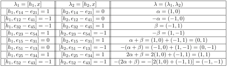
• For B2 ∼=C2, we must showo(5, F)∼=sp(4, F) by adjoining the diagonal matrices from B2, C2 to corresponding eigenvectors to determine the eigenvalues involved in
their respective basis matrices. The diagonal matrices for B2 are as followed:
h1 =e22−e44
Denote λ1 = [h1, x]and λ2 = [h2, x], where x is an eigenvector, then eigenvalue
λ= (λ1, λ2). Recall that [hi, x] =−[hi, xt]
[h1, e21−e14] =h1(e21−e14)−(e21−e14)h1
= (e22−e44)(e21−e14)−(e21−e14)(e22−e44) =e21−e14= 1 [h2, e21−e14] = (e33−e55)(e21−e14)−(e21−e14)(e33−e55) = 0
[h1, e12−e41] =e41−e12=−1 [h2, e21−e14] = 0
Therefore, the eigenvalue for eigenvector e21−e14 is(1,0) =α, and the eigenvalue for eigenvector e12−e41 is(−1,0) =−α. The remaining eigenvalues are derived similarly:
λ1 = [h1, x] λ2 = [h2, x] λ= (λ1, λ2)
[h1, e14−e21] = 1 [h2, e14−e21] = 0 α= (1,0) [h1, e12−e41] =−1 [h2, e12−e41] = 0 −α= (−1,0) [h1, e32−e45] =−1 [h2, e32−e45] = 1 β= (−1,1)
[h1, e23−e54] = 1 [h2, e23−e54] =−1 −β = (1,−1)
[h1, e15−e31] = 0 [h2, e15−e31] = 1 α+β= (1,0) + (−1,1) = (0,1) [h1, e51−e13] = 0 [h2, e51−e13] =−1 −(α+β) = (−1,0) + (1,−1) = (0,−1) [h1, e25−e34] = 1 [h2, e25−e34] = 1 2α+β= 2(1,0) + (−1,1) = (1,1) [h1, e52−e43] =−1 [h2, e52−e43] =−1 −(2α+β) =−[2(1,0) + (−1,1)] = (−1,−1)
Figure 3.2: Table of eigenvalues forB2
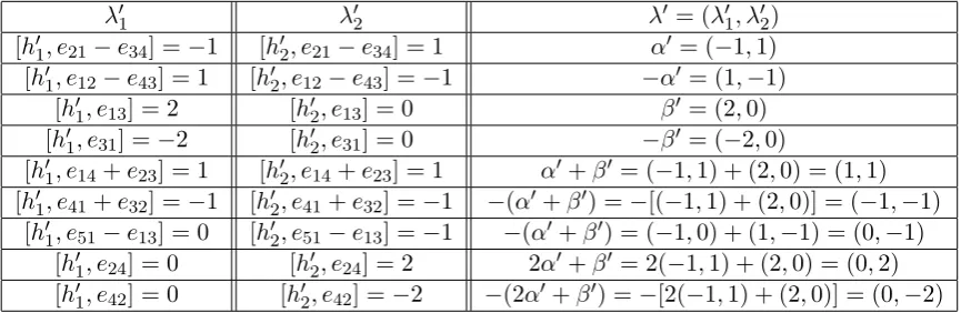
The diagonal matrices for C2 are as followed, wherel= 2:
h01=e11−e33, h02 =e22−e44
Denote λ01 as the eigenvalue of[h01, x]andλ02 as the eigenvalue of [h02, x] where xis
λ01 λ02 λ0 = (λ01, λ02) [h01, e21−e34] =−1 [h02, e21−e34] = 1 α0 = (−1,1) [h01, e12−e43] = 1 [h02, e12−e43] =−1 −α0 = (1,−1)
[h01, e13] = 2 [h02, e13] = 0 β0 = (2,0) [h01, e31] =−2 [h20, e31] = 0 −β0 = (−2,0)
[h01, e14+e23] = 1 [h02, e14+e23] = 1 α0+β0= (−1,1) + (2,0) = (1,1) [h01, e41+e32] =−1 [h02, e41+e32] =−1 −(α0+β0) =−[(−1,1) + (2,0)] = (−1,−1)
[h01, e51−e13] = 0 [h02, e51−e13] =−1 −(α0+β0) = (−1,0) + (1,−1) = (0,−1) [h01, e24] = 0 [h02, e24] = 2 2α0+β0= 2(−1,1) + (2,0) = (0,2) [h01, e42] = 0 [h02, e42] =−2 −(2α0+β0) =−[2(−1,1) + (2,0)] = (0,−2)
Figure 3.3: Table of eigenvalues for C2
We can construct a linear transformation, where
H10 =−1
2h 0 1+ 1 2h 0 2 H 0 2 = 1 2h1+
1 2h2
Let the isomorphism between B2 and C2 be defined by the following map:
α(hi) =α0Hi0 1≤i≤2 β(hi) =β0Hi0 1≤i≤2
Therefore, B2∼=C2, where:
e22−e447→ −12(e11−e33) +12(e22−e44)
e33−e557→ 12(e11−e33) + 12(e22−e44)
e21−e147→
√ 2
2 (e21−e34)
e12−e417→
√ 2
2 (e12−e43)
e32−e457→ e13
e23−e547→ e31
e15−e317→
√ 2
2 (e14+e23)
e31−e417→
√ 2
2 (e41+e32)
e25−e347→ e24
e43−e527→ e42
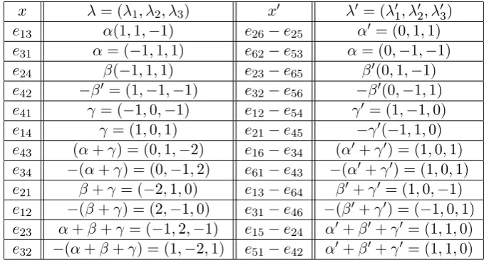
• For A3 ∼=D3, we must showsl(4, F)∼=o(6, F). The diagonal matrices for A3 are:
Denote λ1 = [h1, x], λ2 = [h2, x], andλ3 = [h3, x]. To find the eigenvalue that
corresponds to eigenvector e13, we have:
[h1, e13] = (e11−e22)e13−e13(e11−e22) =e13 [h2, e13] = (e22−e33)e13−e13(e22−e33) =−e13 [h3, e13] = (e33−e44)e13−e13(e33−e44) =−e13
Therefore eigenvalue λ= (λ1, λ2, λ3) corresponding to e13 can be written as
α= (1,−1,−1).
The diagonal matrices for D3 are:
h01 =e11−e44, h02 =e22−e55, h03 =e33−e66
For D3, denote λ01 = [h01, x0], λ02 = [h02, x0], λ03= [h03, x0] where x0 is an eigenvector.
Let λ0 = (λ01, λ02, λ03). The eigenvalues for A3 and D3 are listed on the following
table:
x λ= (λ1, λ2, λ3) x0 λ0 = (λ01, λ02, λ03)
e13 α(1,1,−1) e26−e25 α0= (0,1,1)
e31 α= (−1,1,1) e62−e53 α= (0,−1,−1)
e24 β(−1,1,1) e23−e65 β0(0,1,−1)
e42 −β0 = (1,−1,−1) e32−e56 −β0(0,−1,1)
e41 γ = (−1,0,−1) e12−e54 γ0= (1,−1,0)
e14 γ = (1,0,1) e21−e45 −γ0(−1,1,0)
e43 (α+γ) = (0,1,−2) e16−e34 (α0+γ0) = (1,0,1)
e34 −(α+γ) = (0,−1,2) e61−e43 −(α0+γ0) = (1,0,1)
e21 β+γ = (−2,1,0) e13−e64 β0+γ0 = (1,0,−1)
e12 −(β+γ) = (2,−1,0) e31−e46 −(β0+γ0) = (−1,0,1)
e23 α+β+γ= (−1,2,−1) e15−e24 α0+β0+γ0= (1,1,0)
e32 −(α+β+γ) = (1,−2,1) e51−e42 α0+β0+γ0= (1,1,0) Figure 3.4: Table of eigenvalues forA3 and D3
We can construct a linear transformation:
H10 =−h01+h03, H20 =h01+h02, H30 =−h01−h03
The insomorphism between A3 and D3 is thus obtained by defining a map between
diagonal matrices;
Therefore A3∼=D3, where:
e11−e227→ −(e11−e44) + (e33−e66)
e22−e337→ (e11−e44) + (e22−e55)
e33−e447→ −(e11−e44)−(e33−e66)
e137→ e26−e25
e317→ e62−e53
e247→ e23−e65
e427→ e32−e56
e417→ e12−e54
e147→ e21−e45
e437→ e16−e34
e347→ e61−e43
e217→ e13−e64
e127→ e31−e46
e237→ e15−e24
e327→ e51−e42
3.3
Automorphisms
The set of inner automorphisms of a ring, or associative algebraA, is given by the
conjugation element, using right conjugation, such that:
ϕa:A→A
ϕa(x) =a−1xa
Given x, y∈A:
ϕa(xy) =a−1(xy)a=a−1xaa−1ya= (a−1xa)(a−1ya) =ϕa(x)ϕa(y)
Where, ϕais an (invertible) homomorphism that containsϕ−a1. Thereforeϕa constitutes
an isomorphism onto itself. Since the composition of conjugation is associative,a−1xais
often denoted as xa.
Definition 3.12. An automorphism of L is an isomorphism of L onto itself. AutL
Example 3.3.1. Consider L⊆gl(V), andg∈gl(V) where g is an invertible
endomorphism. Define a mapping φ:L→L0 where xLx−1=L, then x→gxg−1, where
φ is an automophism of L. The same can be said forsl(V) since the trace of a matrix is
invariant under a change of basis.
Example 3.3.2. Let L be a Lie algebra such that L=sl(n, F), g∈GL(n, F). The map
ϕ:L→L defined by x→ −gxtg−1(xt= the transpose of x) belongs to Aut L. When
n= 2, g= the identity matrix, we can prove that AutL is inner.
tr(−gxtg−1) =tr(−gg−1xt) =tr(−xt) =−tr(x) {Sinceg=the identity matrix} ⇒tr(x) = 0⇔tr(−gxtg−1) = 0
Therefore, the map is a linear automorphism of sl(n, F). If we apply the transpose to
the commutator, for x, y∈L, we have:
[x, y]t= (xy−yx)t= (xy)t−(yx)t =ytxt−xtyt= [ytxt]
Therefore:
ϕ[x, y] =−g[x, y]tg−1 =−g[yt, xt]g−1 {By properties of the transpose}
=g(ytxt−xtyt)g−1 =gytxtg−1−gxtytg−1
= [gytg−1, gxtg−1] =gytg−1gxtg−1−gxtg−1gytg−1 = [ϕ(x), ϕ(y)]
Therefore, ϕ is a homomorphism. Thus AutL is inner.
Example 3.3.3. An automorphism of the form exp(adx), with adx nilpotent, i.e.,
(adx)k= 0 for some k >1, is calledinner.
To derive the power series expansion for exp(adx), we begin by constructing the Taylor
series expansion using the differential operator for matrixA. Given an invertible matrix
A, the solution tox0 =A~x might bex0(t) =λveλt. Multiplying byA, we have:
Ax(t) =Aveλt
where λis an eignenvalue ofA with corresponding eigenvectorv. Then the power series
expansion to define eλt when λis complex becomes:
eλt= 1 + (λt) + 1 2!(λt)
2+...+ 1
n!(λt)
n
[Eve66] Let charF = 0, andx∈Lsuch that adx is nilpotent. That is, (adx)k= 0 for
k >0. Then, since adx is finite dimensional, the above series expansion generalizes to:
exp(adx) =
∞
X
k=0
adk(x) k!
= 1 +adx+
(adx)2
2! +
(adx)3
3! +...+
(adx)k−1
(k−1)!
where exp(adx)∈ AutL. To show this, recall that Leibniz’s rule for the product of
derivations is:
δn
n!(xy) =
n
X
i=0 1 i!δ
i(x) 1
(n−1)!δ
n−i(y)
Where δ is an arbitrary nilpotent derivation ofL. Givenx, y∈L:
exp(δ(x))exp(δ(y)) =
n−1
X
i=0
δi(x)
i!
!
n−1
X
j=0
δj(y)
j!
= 2k−2
X
n=0
δn(xy) n!
=
k−1
X
n=0
δn(xy) n!
Where the first equality holds because exp(adx) =P∞k=0 adk
(x)
k! , and the second equality satisfies Leibniz’s product rule. Sinceδ is a nilpotent derivation ofL, the last equality
holds because δk= 0. Therefore, the composition of two inner automorphisms is again an inner automorphism, thus the derivation of an inner automorphisms exp(ad(x)) is a
homomorphism:
[exp(δ(x)), exp(δ(y))] =exp([δ(x), δ(y)])
Where exp δ is invertible by exhibiting the inverse: 1−n+n2−n3+...±nk−1, exp δ =n+ 1. Thus,exp(adx)∈AutL. The subgroup of all such inner automorphisms
Definition 3.13. When adx is nilpotent, the inner automorphism constructed is called
Int L. For φ∈Aut l, x∈L,
φ(adx)φ−1=adφ(x) when φexp(adx)φ−1=exp(adφ(x))
Example 3.3.4. Let σ be the automorphism ofsl(2, F) give by the following: let
L∈sl(2, F), with standard basis (x, y, h). Define σ=exp ad x· exp ad(−y)· exp ad x. We can show that σ(x) =−y, σ(y) =−x, σ(h) =−h. From example 3.1.2, we have [x, y] =h,[h, y] =−2y,[h, x] =−2x
σ(x) =exp adx·exp ad(−y)·exp adx(x) =exp adx·(1 +ad(−y) +ad(−y)
2
2! )x
=exp adx·(x+ (−ady)(x) + 1
2!(ad(−y)) 2(x))
=exp adx·(x−[y, x] + 1
2!(ad(−y))(h)) =exp adx·(x+h+ [−y, h])
= (1 +adx+ad(x) 2
2! )(x+h−y)
= (x+h−y) + ([x, x] + [x, h]−[x, y]) + ([x[x, x]]
2! +
[x,−2x]
2! −
[x, h] 2! )
= (x+h−y) + (−2x−h) + (x) =−y
σ(y) =exp adx·exp ad(−y)·exp adx(y) =exp adx·(1 +adx+ ad(x)
2
2! )(y)
=exp adx·(y+ [x, y] + [x,[x, y]]
2 )
=exp adx·(1 +ad(−y) +ad(−y) 2
2! )(y+h−x) =exp adx·[(y+h−x) + ([−y, y] + [−y, h]−[−y, x]) + ([−y,[−y, y]]
2! +
[−y,[−y, h]]
2! −
[−y,[−y, x]]
2! )]
=exp adx·(y+h−2y−x−h+y) = (1 +adx+ad(x)
2
σ(h) =exp adx·exp ad(−y)·exp adx(h) =exp adx·exp ad(−y)·(1 +adx+ad(x)
2
2! )(h)
=exp adx·exp ad(−y)·(h+ [x, h] + [[x, h], h]
2! )
=exp adx·(1 +ad(−y) +ad(−y) 2
2! )(h−2x)
=exp adx·[(h−2x) + ([−y, h]−2[−y, x]) + ([−y,[−y, h]]
2! )−
2[−y,[−y, x]]
2! )]
=exp adx·[(h−2x) + (−2y−2h) + (0 + 2y)] =exp adx(−h−2x)
= (1 +adx+ ad(x) 2
2! )(−h−2x)
= (−h−2x) + (−[x, h]−2[x, x]) + (−[x,[x, h]]
2 −2
[x,[x, x]]
2 )
Chapter 4
Solvable and Nilpotent Lie
Algebras
4.1
Solvability
In this section, we will decompose L into a collection of subalgebras. GivenL as the
direct sum of ideals, the derivation of Li fori= 1,2...n, consists of a mapping such that the commutator [Li, Li] is zero.
Definition 4.1. The derived series of a Lie algebraL is a sequence of ideals of L where
L0=L, L1 = [LL], L2= [L1L1], ..., Li= [Li−1Li−1].
Given a Lie algebra L, and an ideal I, we have:
[L, I1] = [L,[I, I]]⊆[I,[I, L]] + [I,[L, I]]⊆[I, I] + [I, I] =I1 [Wan75] Therefore, if I is an ideal ofL, then so isI1. Unless otherwise stated, the material for
this chapter is derived from [Hum72].
Example 4.1.1. Given I is an ideal ofL, we can show In+1 is an ideal of L using induction.
Proof. SinceI is an ideal of L,I0=I is also an ideal ofL, as isI1 by the above.
[x[yz]] =−[y[zx]]−[z[xy]] {By the Jacobi identity} ∈[y, In] + [z, In] {Since [z, x],[x, y]∈In} ∈[In, In] + [In, In] {Since y, z ∈In}
∈In+1+In+1
∈In+1
Therefore In+1 is an ideal, making each member of the derived series of I an ideal of L.
Definition 4.2. A group G is said to besolvable if it has a subnormal series
G=G0≥G1≥G2 ≥...≥Gn=e (4.1)
in which the factors Gi/Gi+1 are all Abelian for alli,0≤i≤n−1.
By subnormal, we mean that for each i, 0≤i≤n−1,Gi is normal inGi+1. Given a Lie algebra L, and series lengthn >0 we say that Lis solvable ifL(n)= 0, that is, a Lie algebra is solvable if its derived series terminates in the zero subalgebra. The derived
subalgebra of a finite dimensional solvable Lie algebra over a field of characteristic 0 is
nilpotent, thus making abelian algebras solvable and conversely simple algebras
nonsolvable.
Lemma 4.3. Let 0→J →L→I →0 be an exact sequence of Lie algebras. Then L is solvable if and only if both J and I are solvable. [Sam90]
Proposition 4.4.
1. IfL is a solvable Lie algebra, then so are all of the subalgebras and homomorphic
images of L.
2. IfI is a solvable ideal of L such that the quotient L/I is solvable, then L itself is
solvable.
3. IfI, J are solvable ideals of L, where L is a solvable Lie algebrra, thenI+J is
Proof.
1. Let K be a subalgebra of L, then by definition,K(i) ⊂L(i), therefore K(i) is solvable for all i. If we define a map ϕ:L→M whereϕis an epimorphism, then by induction, we can show ϕ(L(i)) =M(i).
2. Let (L/I)(n)= 0. By construction of the canonical homomorphismπ:L→ L I, we
have thatπ(L(n)) = 0 by part 1. orL(n)⊂I =kerπ. If I(m)= 0, then (L(i))(i) =L(i+j)⇒L(n+m)= 0 (since L(n) ⊂I).
3. By Proposition 3.11 (part 3.): ifI, J are ideals of L, then from the sequence
0→I →I+J → I+JJ →0, there exists a natural isomorphism between the third term (I+J)/J and I/(I∩J). Now (I+J)/J is solvable by the Lemma 4.3, since the homomorphic image of I is solvable. Therefore I/(I∩J) is solvable by part 2.
As a consequence of Proposition 4.4, ifL is solvable, thenLpossesses a unique maximal
solvable ideal, called the radical of L, orRad L. When L issemisimple, RadL= 0.
Recall, Lis simple if it contains no non trivial ideals (i.e., only contains the trivial ideals,
0 and Litself), that is, if RadL= 0. Therefore, every simple algebra is semisimple.
Example 4.1.2. L is solvable if and only if there exists a chain of subalgebras
L=L0 ⊃L1⊃...⊃Lk= 0 such that:
• Li+1 is an ideal ofLi.
• Each quotient Li
Li+1 is abelian.
Proof.
⇒
• Since L is solvable, there exists a sequence of ideals ofL such that
L⊇L(1) ⊇...⊇L(i)= 0 for some i. By definition, each ideal forms a subalgebra of L. By Proposition 4.4, L(i+1)⊆L(i) where L(i+1) and L(i) are ideals ofL.
abelian. By definition of the derived series,L(i+1)= [L(i), L(i)]. Let [x, y]∈L(i+1), with x, y∈L(i):
[x+L(i+1), y+L(i+1)] = [x, y] + [x, L(i+1)] + [L(i+1), y] + [L(i+1), L(i+1)]
= [x, y] +L(i+1)
Therefore LL(i(+1)i) is abelian.
⇐ Given LL(k(−1)k) is abelian andL=L0 ⊃L1 ⊃...⊃Lk= 0, then the derived series forL
terminates in the zero subalgebra. Therefore, by defintion,Lk is solvable, making L
(k−1)
L(k)
solvable, and thus Lk−1 is solvable by Proposition 4.4. Similarly, LLkk−2−1 is solvable, and thusLk−2 is solvable. Continuing this way, LL01 is abelian and thusL1 is solvable. Therefore L0=Lis solvable.
Example 4.1.3. We can show that L is solvable if and only if adL is solvable.
Proof.
⇒ Let L(n) = 0. By induction, whenn= 0,L(0) =L, and adL(0) =adL= (adL)(0).
Therefore adL is solvable for n= 0. Assume adL(n) = (adL)(n),
adL(n+1) =ad[L(n), L(n)] {By definition of the derived series}
= [(adL)(n),(adL)(n)]
Since ad[xy]= [adx, ady]
= (adL)(n+1)
Since Ln+1= [Ln, Ln]
Therefore adL is solvable.
⇐ Since adL is solvable, (adL)(n) =ad(Ln)= 0, by the induction above. Therefore
L(n)⊆Z(L). Therefore ZL(L) is solvable and thus Lis solvable.
4.2
Nilpotency
In this section, we shall explore the descending central series, defined as a recursive
sequence of subalgebras that ends in the zero subspace. We shall rewrite this series
using the quotient space to determine the effect of having a nilpotent algebra as it
Definition 4.5. Thedescending central series is a sequence of ideals of L defined
as L0 =L, L1 = [LL], L2= [LL1], ..., Li = [LLi−1]. We callL nilpotent if for some
n >0, Ln= 0.
Thus Li is spanned bylong brackets [X1[X2[...XI+1]...] (which we abbreviate to [X1X2...Xi+1]) [Sam90]. Notice thatLn= 0 makes any abelian algebra nilpotent. Therefore nilpotent implies solvable since L(i)⊂Li for all i. However solvable does not imply nilpotent.
Example 4.2.1. The algebra n(n, F) of strictly upper triangular matrices is nilpotent.
A matrix is strictly upper triangular if and only if i > j−k. So Given Bijk = 0, implies
Bk= 0 for k≥m if B is an m×m matrix. Using induction, we haveB1= 0 for
i.j−1. Assume Bijk = 0 for i, j−(k−1):
Bkij =BBjk−1=
i
X
r=1
BirBrjk−1+ m
X
r=i+1
BirBrjk−1
=
i
X
r=1
0·Brjk−1+
m
X
r=i+1
Bir·0 = 0
Note that the first term goes to zero, since r≤i where Bir is strictly triangular. The
second term goes to zero since r≥i+ 1>(j−k) + 1 =j−(k−1). Therefore, by the induction step, Bijk = 0.
We can show a similar result for lower triangular matrices using the following indices:
m≥j.i≥1 Cij =Dij = 0
m≥i≥1 Cii=Dii= 0
Which would prove that (CD)ij = 0 [Eve66]
Proposition 4.6.
1. IfL is a nilpotent Lie algebra, then all the subalgebras and homomorphic images
of L are nilpotent.
2. IfL is a Lie algebra such that L/Z(L) is nilpotent, then L is nilpotent.