RESEARCHARTICLE
Mixed map labeling
∗
Maarten Löffler
1, Martin Nöllenburg
2, and Frank Staals
31Department of Information and Computing Sciences, Utrecht University, the Netherlands
2Algorithms and Complexity Group, TU Wien, Vienna, Austria
3MADALGO, Aarhus University, Denmark
Received: October 30, 2015; returned: May 18, 2016; revised: August 23, 2016; accepted: September 14, 2016.
Abstract: Point feature map labeling is a geometric visualization problem, in which a set of input points must be labeled with a set of disjoint rectangles (the bounding boxes of the label texts). It is predominantly motivated by label placement in maps but it also has other visualization applications. Typically, labeling models either use internal labels, which must touch their feature point, or external (boundary) labels, which are placed outside the input image and which are connected to their feature points by crossing-free leader lines. In this paper we study polynomial-time algorithms for maximizing the number of internal labels in a mixed labeling model that combines internal and external labels. The model requires that all leaders are parallel to a given orientationθ∈[0,2π), the value of which influences the geometric properties and hence the running times of our algorithms.
Keywords:algorithms, map labeling, computational geometry, geovisualization
1
Introduction
Annotating features of interest in maps and other images of geographic information with textual labels or graphical icons is an important task in geovisualization. The traditional design principles and quality criteria used in cartographic label placement easily generalize to label placement in arbitrary information graphics and illustrations. In a map, labels are mostly placed internally, that is, touching their respective feature points. Common carto-graphic placement guidelines demand that each label is placed in the immediate neighbor-hood of its feature and that the association between labels and features is unambiguous, while no two labels may overlap each other [16, 27]. Different styles of label placement
∗A preliminary version of this paper appeared in Proc. 9th International Conference on Algorithms and
and their merits have been studied extensively in cartography and geographic information science. However, even when an ideal set of placement rules is agreed upon, it is often not trivial to compute an optimal placement. In the computational geometry literature, there has been extensive work investigating the tractability of different labeling styles. It is known that maximizing the number of non-overlapping labels for a given set of input points isNP-hard, even for very restricted labeling models [10, 23]. In terms of labeling algorithms, several approximations, polynomial-time approximation schemes (PTAS), and exact approaches are known [1, 8, 20, 28], as well as many practically effective heuristics, see the bibliography of Wolff and Strijk [29]. If, however, feature points lie too dense in the map or if their labels are relatively large, often only small fractions of the features obtain a label, even in an optimal solution.
An alternative labeling approach uses external instead of internal labels, which are sometimes known ascallouts. External labels are remotely placed, often outside the image itself, and connected by leaders to their respective feature points. This is known as bound-ary labeling[6] in the algorithmic literature. The boundary labeling style is most frequently used when annotating anatomical drawings [13, 26] and technical illustrations, where dif-ferent and often small parts are identified using labels and longer descriptive texts out-side the actual picture. Other popular applications of boundary labeling are annotation placement in correction mode of word processing software and commenting in document viewers [18]. But also maps and cartographic visualizations can carry external labels, e.g., the Maplex Label Engine in ArcGIS 10.3 offers labels with callouts and leaders.
While the association between points and external labels may be more difficult to see, the big advantages of boundary labeling are that even dense feature sets can be labeled and that larger labels can be accommodated on the margins of the illustration. Many effi-cient boundary labeling algorithms are known. They can be classified by the leader shapes that are used and by the sides of the picture’s bounding box that are used for placing the labels [3, 6, 7, 11, 15, 19, 25]. A recent user study evaluates the readability and aesthetic preference for differently shaped leader types and concludes that, especially for dense fea-ture sets, straight leaders or leaders with at most one bend (horizontal/vertical or horizon-tal/diagonal) perform best [2]. Orthogonal leaders with two bends were clearly outper-formed in most cases.
The combination of internal and external labeling models using internal labels where possible and external labels where necessary seems natural and has been proposed as an open problem by Kaufmann [17]; however, only few results are known in suchhybridor
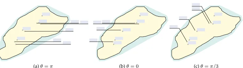
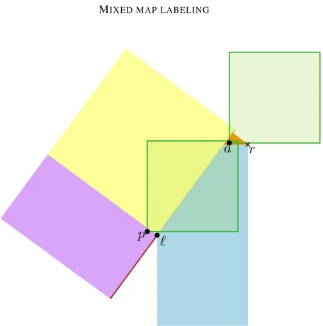
(a)θ=π (b)θ= 0 (c)θ=π/3
Figure 1: A sample point set with mixed labelings of three different slopes. In (a) five external labels are necessary, whereas (b) and (c) require only four external labels. The slope in (c) yields aesthetically pleasing results.
labels and external labels on one or two opposite sides of the bounding box, connected by two-bend orthogonal leaders. Their goal is to maximize the number of internally labeled points, while labeling all remaining points externally. Polynomial and quasi-polynomial-time algorithms, as well as an approximation algorithm and an ILP formulation were pre-sented.
Contribution In this paper, we extend the known theoretical results on mixed map label-ing as follows. We present a mixed labellabel-ing model, in which each point is assigned either an axis-aligned fixed-position internal label (e.g., to the top right of the point) or an external label connected with a leader of slopeθ, whereθ∈[0,2π)is an input parameter defining the unique leader direction for all external labels, measured clockwise from the negativex-axis (see Figure 1). In this model, we present a new dynamic-programming algorithm to maxi-mize the number of internally labeled points for any given slopeθ, including the left- and right-sided case (θ= 0orθ=π), which was studied by Bekos et al. [4]. While for the right-sided case Bekos et al. provided a fasterO(nlog2n)-time algorithm, wherenis the number of input points, our algorithm improves upon their pseudo-polynomial O(nlogn+3)-time
algorithm for the left-sided case. We solve this problem in O(n3(logn+δ))time, where
δ = min{n,1/dmin} is the inverse of the distancedmin of the closest pair of points in P
and expresses the maximum density ofP (Section 2). In the general case it turns out that the set of slopes can be partitioned into twelve intervals, in each of which the geometric properties of the possible leader-label intersections are similar for all slopes. Depending on the particular slope interval, the amountι(n, δ, θ)of “interference” between sub-problems varies. This significantly affects the algorithm’s performance and leads to running times betweenO(n3logn)andO(n3(logn+ι(n, δ, θ))) ⊆ O(n7)(Section 3). From a theoretical
point of view, this shows that mixed map labeling can be solved optimally in polynomial time for any leader slope. From a practical point of view, near-cubic running times up to
O(n7)(depending on the leader slope) seem too slow at first sight. However, in many
internal labels over all slopesθ at an increase in running time by a factor ofO(n2), as is
shown in Section 4.2.
Problem statement We are given a map (or any other illustration)M, which we model for simplicity as a convex polygon (this is easy to relax to larger classes of well-behaved domains), and a setP of npoints in Mthat must be labeled by rectangular labels (the bounding boxes of the label texts). In addition, we are given a leader slopeθ∈[0,2π). For simplicity we assume thatθis none of the slopes defined by two points inP. We discuss in Section 4.6 how to remove this restriction. There are two choices for assigning a label to a pointp∈ P: either we assign aninternal labelλponMin a one-position model, or an external labeloutside ofMthat is connected topwith a leader γp. An internal labelλpis a rectangle that is anchored atpby its lower left corner. A leaderγp is a line segment of slopeθinsideM; it may bend to the horizontal direction outside ofMin order to connect to its horizontally aligned label, see Figure 1c. So in this model, the labeling is fixed once the choice for an internal or external label has been made for each pointp∈ P. For avalid
label assignment we require that (i) the labels do not overlap each other or the leaders, and that (ii) the leaders themselves do not intersect each other. As we will see in Section 4.4 it is easy to realize constraint (i) for the external labels. Figure 1 shows valid mixed labelings for three different slopes.
Given a set of pointsP⊆ P, letΛ(P) ={λp|p∈P}denote the set of (candidate) labels corresponding to the points inPand letΓ(P) ={γp |p∈P}denote the set of (candidate) leaders corresponding to the points inP. AlabelingofP is a partition ofPinto setsI and
E, the points inI labeled internally, the points in E labeled externally, such that no two labels inΛ(I)intersect, no two leaders inΓ(E)intersect, and no label fromΛ(I)intersects a leader fromΓ(E).
For ease of presentation we first assume that all labels have the same size, which, with-out loss of generality, we assume to be1×1, but the problem can be solved with the same algorithms for rectangular labels of any other fixed size and shape. Hence, an internal label
λpis a unit square with its bottom left corner onp. This may be a realistic model in some settings (e.g., unit-size icons as labels [14]), but generally not all labels have the same size. We will sketch how to relax this restriction in Section 4.5.
Each leaderγpcan be split into aninnerpart (orinner leader), which is a line segment of slopeθfrompto the intersection point with the boundary ofM, and anouterpart (orouter leader) from the boundary ofMto the actual label. In this paper we focus our attention on the inner leaders as they determine howP is separated into different subinstances. Hence we can basically think of the leaders as half-lines with slopeθ. Again, this assumption is not realistic for mixed map labeling in practice, where the placement of labels and the routing of leaders outside of M is an important sub-problem. We explain a simple method of routing the outer leaders in Section 4.4 and discuss possible consequences and approaches if the space for external labels is bounded. Studying this external labeling problem in its entirety is beyond the scope of this paper and gives rise to computational problems of independent interest.
an anchor point and then applying a simple greedy algorithm on the resulting staircase patterns [21]. On the other hand, it is also known that any instance can be labeled with external labels using efficient algorithms [5, 6]. Mixed labelings combine both label types and sit between the two extremes of purely internal and purely external labeling [4, 21]. Here we are interested in the internal label number maximization problem, which was first studied forθ ∈ {0, π} by Bekos et al. [4]: Given a mapM, a set of pointsP inMand a slopeθ∈[0,2π), we wish to find a valid mixed labeling that maximizes the number|I|of internally labeled points.
2
Leaders from the left
We start with the case thatθ= 0, i.e., all leaders are horizontal half-lines leading from the points towards the left ofM. Our approach for maximizing the number of internal labels is to process the points inP from right to left and to recursively determine the optimal rightmost unprocessed pointpto be assigned an external label. Since no leader may cross any internal label, the leaderγpdecomposes the current instance left ofpinto two (almost) independent parts, one aboveγpand one below. As it turns out, a generic subinstance can be defined by an upper and a lower leader shielding it from the outside and additional information about at most one point outside the subinstance. The problem is then solved using dynamic programming.
2.1
Geometric properties
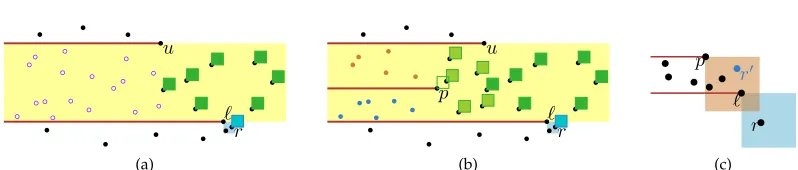
In this section we prove that the problem has a certain geometric structure that we can use to obtain an efficient algorithm. In particular, we show that if we consider a horizontal slab defined by two points`anduas shown in Figure 2, the points in the purple region are shielded from the labels and leaders of the points outside of the horizontal slab by the leaders of the points`andu. In such a configuration, there can be at most one point
routside the slab, i.e., outside the purple and yellow region, whose label or leader may interfere with the labeling of the points in the purple region. Such a pointrmust lie in the unit square whose top-left corner is`(the blue region in Figure 2).
Letp = (px, py)be a point in the plane and let Lp = {q | qx < px} and Rp = {q | qx > px} denote the half-planes containing all points strictly to the left and to the right ofp, respectively. Analogously, we define the half-planesTp andBpabove and belowp, respectively. LetS(`, u) = T`∩Bu denote the horizontal slab defined by points` andu (with`y < uy), and letS(`, u) =S(`, u)∩L`∩Ludenote the set of points in this slab that lie to the left of both`andu, see Figure 2(a). We defineP`,uas the subset ofP inS(`, u) including`andu, i.e.,P`,u =P ∩(S(`, u)∪ {`, u}). With some abuse of notation we will sometimes also useLp,Rp,Tp, andBpto mean the subset ofP that lies in the respective half-plane rather than the entire half-plane.
Recall thatδ= min{n,1/dmin}is a parameter that captures the maximum density ofP
as the inverse of the smallest distancedminbetween any two points inP. We can useδto
bound the number of candidate points in a unit square that may be labeled internally.1
1Since all internal labels are unit squares, any unit square can have only one point that is labeled internally. We
u
`
(a)
` z
b E(`)
(b)
Figure 2: (a) The slabS(`, u)in yellow, the regionS(`, u)and its points fromP in purple, and the regionE(`)in blue. (b) An enlarged view of the regionE(`).
Lemma 1. At mostO(δ)points in any unit square have a label λthat does not contain another point inP.
Proof. LetEbe a unit square and letEP =E∩Pbe the input points inE. Since the labelλp of every pointp∈EP is a unit square anchored by its lower left corner atp, no other point q ∈ P may lie to the top-right ofp—otherwisepmust be labeled externally. Hence any set of points inEP whose labels do not contain another point ofP must form a sequence p(1), p(2), . . . , p(k) such thatp(i)
x < p(xj) andpy(i) > p(yj)for any i < j. Since the minimum distance of any two points isdminwe immediately obtain thatEP contains at mostO(δ)
points whose label does not contain another point inP.
Next, we characterize which leaders or labels outside of S(`, u) can interfere with a potential labeling ofP`,uassuming that`anduare labeled externally.
Lemma 2. Let`, u ∈ P, let(I0,E0), with`, u ∈ E0 be a labeling ofP
`,u. There is no point in Tu∪B`whose leader intersects a label fromΛ(I0)and there is no point inTuwhose label intersects a label fromΛ(I0).
Proof. In any labeling ofP`,uthere are no intersections between labels and leaders. In par-ticular, no labelλpforp∈ I0intersectsγ`orγu. It follows that all labels forI0lie inside the slabS(`, u). By definition, all leaders forE0 also lie insideS(`, u). Since leaders of points
inTu∪B`do not intersectS(`, u), no such leader can intersect a label fromI0. Moreover, all labels are anchored by their bottom left corner, and hence all labels of points inTu lie aboveuand do not intersectS(`, u). Thus, no label for a point inTucan intersect a label in Λ(I0).
It is not true, however, that labels for points inB`cannot intersect labels forP`,u. Still, the influence ofB`is very limited as the next lemma shows. LetE(`)denote the open unit square with top-left corner`, i.e.,E(`) = R`∩B`∩Lz∩Tb, wherez = (`x+ 1, `y)and b= (`x, `y−1). See Figure 2(b).
Lemma 3. Let`, u∈ P, let(I0,E0), with`, u∈ E0be a labeling ofP
`,u, and let(I00,E00)denote a labeling ofP ∩B`∪ {`}with`∈ E00. There is at most one pointp∈ I00whose label may intersect a label ofI0, andp∈E(`).
Proof. Since` ∈ E0 ∩ E00 we know that no label inΛ(I0)orΛ(I00) intersectsγ
of points whose labels intersect a label ofI0, and letΛ(P00)denote the corresponding set of
labels. We first argue thatP00⊆E(`). Then we argue thatP00can contain at most one point.
The labels inΛ(P00)do not intersectγ
`, hence they lie strictly right of`. Thus,P00⊆R`. All points inI0 lie to the left of`, and their labels have width one. All labels inΛ(P00)
intersect such a label, thus all points in P00 must lie inL
z, wherez = (`x+ 1, `y). All labels inΛ(P00)intersect a label from a point inI0. Thus, all labels inΛ(P00)intersect the
horizontal line containingγ`. Since all labels have height one, it follows that all points in P00lie inT
b, whereb = (`x, `y−1). By definition the points inP00lie inB`. So we have P00⊆R
`∩Lz∩Tb∩B`=E(`).
The labels inΛ(P00)are pairwise disjoint and all intersect the top sidesofE(`). Since
the length ofsis smaller than one, each label inΛ(P00)has width exactly one, and all labels
lie inR`it follows that there can be at most one label inΛ(P00). Thus, there is also at most one point inP00.
From Lemma 2 and Lemma 3 it follows that if`anduare labeled externally, there is at most one pointrbelow`that can influence the labeling of the points inS(`, u).
2.2
Computing an optimal labeling
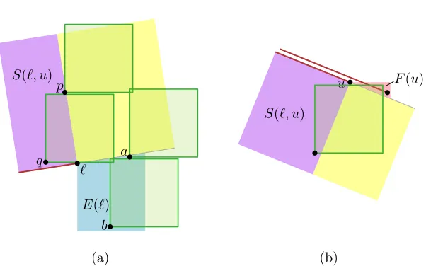
Using the result from the previous section, we now show that the rightmost point that is labeled externally decomposes the problem into two almost independent smaller sub-problems. We can use this to compute an optimal labeling efficiently. Consider again a horizontal slab defined by points`andu, as shown in Figure 3, and assume that pointr
in the blue region is labeled internally. The key idea is then that if we guess the rightmost pointpfrom the slab labeled internally, then we can compute an optimal solution for the points in the slab by combining optimal solutions for two smaller sub-problems. Namely, the sub-problem defined by`,p, andr(the blue points from Figure 3(b) in the slab defined by`andp), and the sub-problem defined bypanduand an appropriate pointr0(the orange points from Figure 3(b) in the slab defined bypandu). This means that we can express the number of points that can be labeled internally as a recursive functionΦ, parameterized by three points:`,u, andr.
We compute the valuesΦ(`, u, r) by dynamic programming. When we combine the solutions Φ(`, p, r) and Φ(p, u, r0) of smaller sub-problems into a solution for the larger
sub-problemΦ(`, u, r)(i.e., a solution for our slab as defined above) we have to test if all labels of points right ofpare free of intersections. We show that we can precompute this information using a sweepline algorithm.
We defineΦ(`, u, r), with`, u ∈ P, andr ∈ E(`)∪ {⊥}as the maximum number of points inS(`, u)that can be labeled internally, given that
(i) the points`anduare labeled externally,
(ii) all remaining points inS(`, u)\S(`, u)have been labeled internally, and
(iii) pointris labeled internally. Ifr=⊥then no point inE(`)is labeled internally.
u
` r
(a)
u
` p
r
(b)
r
r0
` p
(c) Figure 3: (a)Φ(`, u, r)expresses the maximum number of points inS(`, u)(white marks with purple outline), that can be labeled internally in the depicted situation. (b) The right-most pointpthat is labeled with an external label decomposes the problem into two sub-problems (the orange and blue points). (c) Pointr0 =%(p, `, r)(blue) is the topmost point
fromT`∪ {r}that lies in the regionE(p)(the orange unit square).
Lemma 4. For any `, u ∈ P, andr ∈ E(`)∪ {⊥}, we have that Φ(`, u, r) = |S(`, u)|, or
Φ(`, u, r) =|Rp∩S(`, u)|+ Φ(`, p, r) + Φ(p, u, r0), wherepis the rightmost point inS(`, u)with an external label andr0=%(p, `, r).
Proof. Let(I∗,E∗)be an optimal labeling ofS(`, u)that satisfies the constraints(i)–(iii)on
Φ(`, u, r), i.e.,Φ(`, u, r) =|I∗|. In caseE∗=∅, we haveΦ(`, u, r) =|S(`, u)|and the lemma
trivially holds. Otherwise, there must be a rightmost pointp∈ E∗with an external label.
Consider the partition ofI∗at pointpinto the lower left partB∗=B
p∩Lp∩ I∗, the upper left partT∗ =Tp∩Lp∩ I∗, and the right partR∗=Rp∩ I∗, see Figure 3b. We show that |R∗|=|Rp∩S(`, u)|,|B∗|= Φ(`, p, r), and|T∗|= Φ(p, u, r0), which proves the lemma.
Sincepis the rightmost point with an external label it follows that all points inS(`, u) right ofpare labeled internally. Hence,R∗=Rp∩S(`, u).
Next, we observe thatLB = (B∗, S(`, p)\B∗)as a sub-labeling of(I∗,E∗)forms a valid labeling ofS(`, p), so by Lemma 3 there is at most one pointrˆbelow`that can influence the labeling ofS(`, p). This pointˆr, if it exists, lies inE(`). By constraint(iii)pointrlies in
E(`)orr=⊥and no point inE(`)is labeled internally, and thusrcan be the only point in
E(`)labeled internally, i.e.,rˆ=r. So, we have that(i)`andpare labeled externally,(ii)all points inS(`, p)\S(`, p)are labeled internally, and(iii)pointris the only internally labeled point inE(`). Thus the definition ofΦapplies and we obtain|B∗| ≤Φ(`, p, r).
Lemmas 2 and 3 together imply that any labeling ofS(`, p)is independent from any labeling ofS(p, u). Thus, it follows that LB is an optimal labeling of S(`, p)(given the constraints), since otherwise(I∗,E∗)could also be improved. Thus|B∗| ≥ Φ(`, p, r)and
we obtain|B∗|= Φ(`, p, r).
Finally, we consider the upper left partT∗. By Lemma 3 there is at most one pointr0in
Bpwith an internal label that can influence the labeling ofS(p, u)and we haver0 ∈E(p). We need to show thatr0 = %(p, `, r). Then the rest of the argument is analogous to the argument forB∗.
We claim thatr0 is the topmost point inE(p)∩(T`∪ {r}). Assume thatr0 6∈T`, which meansr0 ∈ B
`. We know thatγ` does not intersectλr0 and hencer0 ∈ R`. This means
thatr0 ∈ E(p)∩B
`∩R` =: X and sinceplies to the top-left of`we haveX ⊆ E(`). By definitionris the only point with an internal label inE(`)and hencer0 =r. So ifr0 6= r
we haver0 ∈ E(p)∩T
E(p)can be labeled internally. This is a contradiction since by definitionpis the rightmost externally labeled point in S(`, u)and by constraint(ii) all points in S(`, u)\S(`, u)are labeled internally. So indeedr0 =%(p, `, r)and the same arguments as forB∗can be used to obtain|T∗|= Φ(p, u, r0).
Let`,u∈ P, andp∈S(`, u). We observe that|S(`, p)|and|S(p, u)|are strictly smaller than|S(`, u)|. Thus, Lemma 4 gives us a proper recursive definition forΦ:
Φ(`, u, r) = max
Ψ(S(`, u)),
max
p∈S(`,u){Ψ(Rp∩S(`, u)) + Φ(`, p, r) + Φ(p, u, %(p, `, r))} ,
where
Ψ(P) =
|P| if all labels inΛ(P∪{r}∪(S(`, u)\S(`, u)))are pairwise disjoint,
and their intersection withγ`andγuis empty, −∞ otherwise.
We can now express the maximum number of points inPthat can be labeled internally usingΦ. We add two dummy points toP that we assume are labeled externally: a point
p∞that lies sufficiently far above and to the right of all points inP, and a pointp−∞below and to the right of all points inP. The maximum number of points labeled internally is thenΦ(p−∞, p∞,⊥).
ComputingΦ(`, u, r). We use dynamic programming to computeΦ(`, u, r)for all`, u ∈ P ∪ {p∞, p−∞}with`y < uyandr∈E(`)∪ {⊥}. By finding the maximum in a set of size O(n), each valueΦ(`, u, r)can be computed inO(n)time, given that the valuesΦ(`0, u0, r0)
for all sub-problems have already been computed and stored in a table and the relevant values for the functions%andΨhave been precomputed. There areO(n)choices for each of`andu; further there areO(δ)choices for the pointrgiven`sinceris labeled internally and we know from Lemma 1 that there are at mostO(δ)points inE(`)as candidates for an internal label. We assume theO(δ)candidate points inE(`)are stored; note that we can easily precompute these sets for all points`inO(n2)time. This results in anO(n3δ)time
andO(n2δ)space dynamic-programming algorithm. We show next that the preprocessing
of%andΨcan be done inO(n3logn)time.
Computing %and Ψ. To computeΦ(`, u, r) we actually have to compute%(p, `, r)and Ψ0(p, r) := Ψ(R
p∩S(`, u))for all pointsp∈ S(`, u). We can preprocess all points inP in O(nlogn)time, such that we can compute each%(p, `, r)inO(1)time as follows. First, we compute and store for each pointp∈ Pthe topmost pointqp ∈ P inE(p). This requiresn standard priority range queries that takeO(nlogn)time in total using priority range trees with fractional cascading [9, Chapter 5]. To compute%(p, `, r)we then check ifqplies above `. If it does, we have%(p, `, r) = qp. Otherwise, the only candidate point for%(p, `, r)isr and we can check inO(1)time ifrlies inE(p). This takesO(1)time for each triple(p, `, r) andO(n2δ)time in total.
Next, we fix`andu, and compute a representation ofΨ0inO(nlogn)time, such that
for eachp∈S(`, u)andr∈E(`)∪ {⊥}we can obtainΨ0(p, r)in constant time.
We start by computing the valuesΨ0(p,⊥), for allp. We sweep a vertical line from right
points in that order. The status structure of the sweep line contains the number of points
N inS(`, u)to the right of the sweep line, and a (semi-)dynamic data structureT, which stores the labels from the points to the right of the sweep line, and can report all labels intersected by an (axis-parallel) rectangular query window. All labels are unit squares, so
λr intersects a label λq if and only if λrcontains a corner point ofλq. Furthermore, we only ever insert new labels (points) intoT, thus it suffices ifT supports only insert and query operations. It follows that we can implementT using a semi-dynamic range tree using dynamic fractional cascading [24]. In this data structure insertions and queries take
O(logn)time.
When we encounter a new pointp,p6∈ {`, u}we test if the label ofpintersects any of the labels encountered so far. We can test this using a range query in the treeT. Ifp∈S(`, u) we also explicitly test ifλp intersects γ` orγu. If there are no points in the query range λp, andλpdoes not intersectγ`orγuwe reportΨ0(p,⊥) =N, incrementN (if applicable), and insert the corner points ofλpintoT. If the query rangeλpis not empty, it follows that Ψ0(p0,⊥) =−∞, forp0 =pas well as for any point to the left ofp. Hence, we report that and stop the sweep. Our algorithm runs inO(nlogn)time: sorting all points takesO(nlogn) time, and handling each of theO(n)events takesO(logn)time.
Now consider a pointr∈E(`). We observe that for all pointspright ofr, we have that Ψ0(p, r) = Ψ0(p,⊥) = 0sinceris right of all points inS(`, u). Consider the points left ofr
ordered by decreasingx-coordinate. There are two options, depending on whether or not
λrintersects the labelλpof the current pointp. Ifλrintersectsλp, we haveΨ0(p, r) =−∞ as well asΨ0(p0, r) =−∞for all pointsp0left ofp. Ifλ
rdoes not intersectλpwe still have Ψ0(p, r) = Ψ0(p,⊥). We can test ifλ
rintersects any other label using a range priority query withλrin (the final version of) the range treeT. We needO(δ)such queries, which take O(logn)time each. This gives a total running time ofO(nlogn). We then conclude:
Lemma 5. Given points `, u ∈ P, we can computeΨ0(p, r)for all points p ∈ S(`, u)and all r∈E(`)inO(nlogn)time.
The above algorithm can also be used when the leaders have a slopeθ 6= 0. However, the data structureT that we use is fairly complicated. In this specific case whereθ= 0, we can also use a much easier data structure, and still get a total running time ofO(nlogn). Instead of using the semi-dynamic range tree as status structure, we use a simple balanced binary search tree that stores (the end-points of) a set of verticalforbidden intervals. When we encounter a new pointp, we check ifpylies in a forbidden interval. If this is the case thenλpintersects another label. Otherwise we can labelpinternally. This set of forbidden intervals is easily maintained inO(logn)time.
We use this algorithm for every pair(`, u). Hence, after a total ofO(n3logn)
preprocess-ing time, we can answerΨ0(p, r)queries for anypandrin constant time. This yields the fol-lowing result, which improves the previously best known pseudo-polynomialO(nlogn+3)
-time algorithm of Bekos et al. [4] for the left-sided caseθ= 0.
Theorem 6. Given a setPofnpoints, we can compute a labeling ofPthat maximizes the number of internal labels forθ= 0inO(n3logn+n3δ)time andO(n2δ)space, whereδ= min
{n,1/dmin}
` a
b q
S(`, u)
p
(a)
u
S(`, u)
(b)
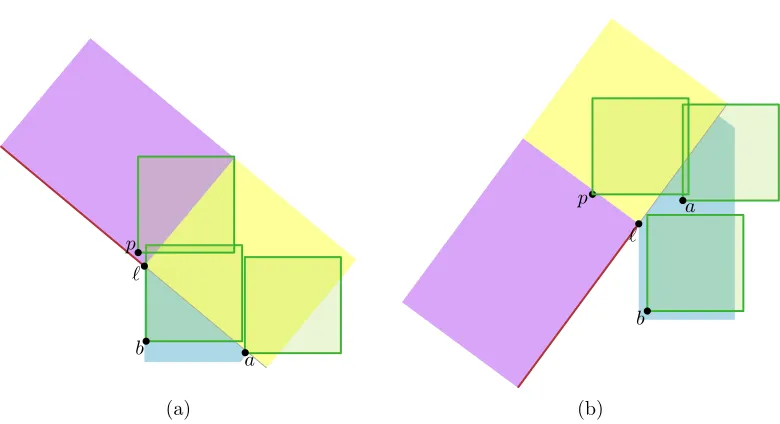
E(`)
F(u)
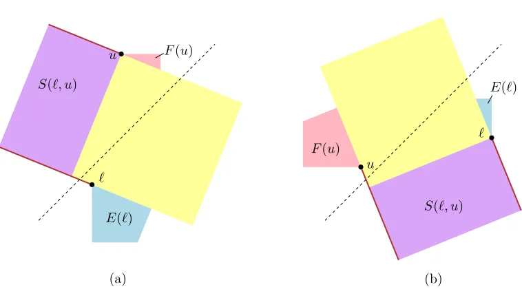
Figure 4: (a) There may be more than one point “below” ` with an internal label if the leaders arrive from the bottom left. (b) For other directions there is also a region F(u) “above” the sub-problem that can influence the labeling ofS(`, u).
3
Other leader directions
For other leader slopesθ 6= 0 we use a similar approach as before. We consider a sub-problemS(`, u)defined by two externally labeled points`andu. We again find the “right-most” point in the slab labeled externally. This gives us two sub-problems, which we solve recursively using dynamic programming. However, there are three complications:
• The regionE(`)containing the points “below” the slabS(`, u)that can influence the labeling ofS(`, u)is no longer a unit square. Depending on the orientation, it can contain more than one point with an internal label. See Figure 4(a).
• In addition to the regionE(`), which contains points that can interfere with a sub-problem from below, we now also need to consider a second region, which we call
F(u), containing points whose labels can interfere with a sub-problem from above. See Figure 4(b).
• The labels of points inS(`, u)are no longer fully contained in the slabS(`, u). Hence, we have to check that they do not intersect with leaders of points outsideS(`, u). See Figure 4(b).
We start by explicitly finding the points inPwhose internal labels contain other points. We are forced to label these points externally. It is easy to find those points inO(n2)time
in total. LetPXdenote this set of points. Additionally, we spendO(n2)time to mark each point if its label intersectsΓ(PX). Hence, for each point we can determine in constant time if it intersectsΓ(PX). For ease of notation we will writeP to mean the setP \ PX in the remainder of this section.
half-planes bounded bypwith respect to this coordinate system. Analogously, we define
S(`, u) = ˜T`∩B˜u, andS(`, u) =S(`, u)∩L˜`∩L˜u.
Our goal is again to bound the number of different labelings of the points inB˜` and ˜
Tu that can influence the labeling ofS(`, u). We will show that whether a labeling ofB˜` influences the labeling ofS(`, u)depends only on a small subset of the points inB˜`. We refer to a labeling ofB˜`restricted to those points as aconfigurationofB˜`. The same holds for the points inT˜u.
3.1
Bounding the number of configurations
Before we solve the problem for arbitrary orientations, we first investigate what structural changes we encounter as we rotate through the full circle of possible orientations. Since we assume that labels are always placed to the top right of the points and are square shaped, it follows that the behavior of the problem is symmetric in leader directions to the top left and directions to the bottom right of the main diagonalx=y. (Remember that the square labels are not a restriction; see Section 4.5.) Hence, the problem for leaders leading down is symmetric to the problem for leaders leading to the left, and can be solved using the same algorithm as described in the previous section.
As we rotate the leader direction, we encounter structural changes whenever the leader angle is a multiple of45◦. This is illustrated in the “wheel of direction” in Lemma 7 and in Figure 5. Specifically, we now define two regionsEandF analogous toEin the previous section; these regions contain all points whose placement influences the solution of a sub-problem. The number of points that can be labeled internally inEandFdirectly influences the running time, since we need to try all possibilities. Figure 5 illustrates the shape ofE
(the shape ofF is symmetric by reflection in the linex=y, see Figure 7).
An additional complication is that the labels of points in S(`, u) are no longer fully contained in the slab defined by`andu. This means that they could potentially intersect with leaders of points outside the slab, whose state we do not yet know when solving the sub-problem. We prove that the number of ways the solution can influence the situation outside the slab in this way is only linear.
We start by bounding the number of configurations ofB˜`. LetE(`)denote thebottom influence regionof`. That is, the points inB˜`“below” the slabS(`, u)whose labels can in-tersect a label of a point inS(`, u). Figure 5 shows the regionsE(`)for various orientations of the leaders.
Similarly, we can define a regionE0(`)⊂B˜`such that theleadersof points inE0(`)can
intersect a label of a point inS(`, u).
Lemma 7. For a sub-problemS(`, u)the size of the bottom influence regionE(`)is at most1×e(θ)
ore(θ)×1, where
e(θ)≤
1 ifθ= 0 2 ifθ∈(0, π/4) 1 ifθ∈[π/4, π/2) 0 ifθ=π/2 1 ifθ∈(π/2,3π/4)
e(θ)≤
0 ifθ∈[3π/4,5π/4] 1 ifθ∈(5π/4,3π/2) 0 ifθ= 3π/2 3 ifθ∈(3π/2,7π/4) 2 ifθ∈[7π/4,2π).
θ
1 2
2
3 0 1
`
θ= 0 1×1
`
1×2
θ∈(0, π/4)
`0 r0
r
p
`
1×1
θ∈[π/4, π/2)
`0
`
θ=π/2 –
`0 1
`
1×1
θ∈(π/2,3π/4)
`0 1
1
`
–
θ∈[3π/4, π)
`
θ=π
–
`
–
θ∈(π,5π/4]
`
1×1
θ∈(5π/4,3π/2)
`0
`
θ= 3π/2 –
`
3×1
θ∈(3π/2,7π/4)
`0
r p
`
2×1
θ∈[7π/4,2π)
`0
Proof. We prove this by case distinction onθ. (See also Figure 5)
caseθ= 0. See Lemma 3.
caseθ∈(0, π/4). All labels inΛ(S(`, u))lie inT`and inL˜r, wherer= (`x+1, `y). It follows thatE(`)⊆T`0∩L˜r0, where`0= (`x, `y−1)andr0= (rx, ry−1). Furthermore, it is easy
to see thatE(`)⊂R`, and thatE(`)⊆B˜`. Hence,E(`)⊂T`0∩R`∩L˜r0 ∩B˜`.
Since the leaders are sloped downwards it follows that the height ofE(`)is at most one. The maximum width ofE(`) is realized by` and the intersection pointpof the lines boundingB˜`andL˜r0. Using thatθ∈(0, π/4)basic trigonometry shows that the width is
at most two.
caseθ ∈[π/4, π/2). Similar to the previous case. However, now the width is determined by the intersection betweenT`0 andB˜`. From basic trigonometry it then follows that the
width is at most one.
caseθ =π/2. For labels fromE(`)to intersectΛ(S(`, u))we needE(`) ⊆T`0, where`0 =
(`x, `y −1). However, to avoid intersecting γ` we need E(`) ⊆ B`0. It follows that E(`) =∅.
caseθ∈(π/2,3π/4). Using similar arguments as before it follows thatE(`)⊂B`0 ∩L˜`0 ∩
˜
B`∩L`∩R`0, where`0 = (`x−1, `y−1). SinceE(`)⊂L`∩R`0 the width is at most one.
Basic trigonometry again shows that the height is at most one.
caseθ ∈[3π/4,5π/4]. For the sub-caseθ ∈[3π/4, π)the lines boundingL˜` andR`0, with `0 = (`x−1, `y−1)intersect below the line containingγ`. We then obtainE(`)⊂R`0 ∩ B`0 ∩B˜` = ∅. In the remaining sub-caseθ ∈ [π,5π/4]the regionsΛ(S(`, u))andΛ( ˜B`)
are disjoint. It follows thatE(`)is empty.
caseθ ∈ (5π/4,3π/2). Point`is now the point with the maximum y-coordinate. It then follows that all labels ofS(`, u)lie inB`0, where `0 = (`x, `y+ 1). Hence, we also get E(`)⊂B`0. The labels ofS(`, u)do not intersectγ`, hence they are contained inL`∪T˜`.
We then haveE(`)⊂B˜`∩(L`∪T˜`) = ˜B`∩L`. Sinceθ∈(5π/4,3π/2)it now follows that the height and width are both at most one.
caseθ = 3π/2. All labels fromS(`, u)lie inL`, all labels fromB˜` = R` lie inR`. Hence, E(`) =∅.
caseθ∈(3π/2,7π/4). It is again easy to show thatE(`)⊂R`∩Lr, wherer= (`x+1, `y+1), and thus has width (at most) one. All labels from points inS(`, u)have width and height one, and are thus contained inL˜r. Furthermore, they do not intersectγ`, from which we obtain that they are contained inT˜`∪T`. From the former we get thatE(`) ⊂ L˜r. From the latter we get thatE(`)⊂ T˜`0 ∪T`0, where`0 = (`x, `y−1). Hence, we obtain E(`)⊂R`∩Lr∩L˜r∩( ˜T`0∪T`0)∩B˜`.
Sinceθ∈(3π/2,7π/4)the height ofE(`)is determined by`0and the intersection pointp
betweenB˜`andL˜r. Trigonometry now shows that the height is at most three.
caseθ∈[7π/4,2π) Similar to the previous case we get a width of at most one. The height is now determined by`0 and the intersection ofB˜`andRr. Sinceθ∈[7π/4,2π)the height is at most two.
Corollary 8. There can be at moste(θ)points inE(`)labeled internally such that their labels are disjoint.
Next, we turn our attention to the points inE0(`) whose leader can intersect a label
` z S(`, u)
p
qR qL `0
p
` z
S(`, u)
(a) (b)
Figure 6: The regionE0(`)(in orange) for the casesθ ∈(5π/4,3π/2)(a) andθ∈(3π/2,2π)
(b). In both cases the leaderγpof a pointp∈E00(`)intersects the line segment`zand thus subdividesE(`)into a left regionLand a right regionR.
(3π/2,2π), see Figure 5. In the former case we thus have E0(`) = ˜B
`∩T˜`0 ∩L`, where `0 = (`
x, `y+ 1−tan(θ−5π/4)), and in the latter case we haveE0(`) = ˜B`∩T˜z∩Tz, where z= (`x+ 1, `y), see Figure 6.
We now note that if we label the setQ ⊆E(`)internally, then all other points inE(`) are labeled externally. Hence, if the leaders of the remaining points (e.g., those inE(`)\
Q) intersect with labels of points inS(`, u), this is already captured by the configuration involvingQ. Therefore, the points inE(`)\Qthemselves do not define new configurations. Similarly, the points that we were forced to label externally, the setPX, do not define any new configurations.
The points inE0(`)that lie outside ofE(`)can still be labeled both internally or
exter-nally. LetE00(`) =E0(`)\E(`)denote the region containing these points. We now observe:
Lemma 9. Let Q be the set of points in E(`)labeled internally, and letp ∈ E00(`)be labeled externally. For all points q ∈ Qwe have: λq intersects the leader γp, or if there is a label λa, a∈S(`, u), that intersectsλq, then it also intersects the leaderγp.
Proof. It is easy to see that any leaderγpintersects the line segment`z, withz= (`x, `y+ 1) ifθ ∈ (5π/4,3π/2), andz = (`x+ 1, `y)if θ ∈ (3π/2,2π), see Figure 6. In both casesγp subdividesE(`)into a left regionLand a right regionR. At any height (y-coordinate), this left regionLhas width at most one. Hence, if there is a pointq∈Llabeled internally, then its label intersectsγp. Any pointq∈Ris separated fromS(`, u)byγp. So, if there is a label a∈S(`, u)that intersectsλq, then it also intersectsγp.
Observation 10. Letp∈ P ∩E00(`)be the point closest to the slabS(`, u), and letqbe any point inP ∩E00(`). If there is a pointa∈S(`, u)whose labelλ
aintersectsγq, thenλaalso intersectsγp. Observation 10 gives us that there is only one relevant point inE00(`), namely the point pclosest toS(`, u). Furthermore, from Lemma 9 it follows that ifpexists, then there are no relevant points inE(`)labeled internally. Hence,pby itself determines a configuration. We can then define the universeU`Eof possible configurations ofB˜`as follows:
(a)
u
S(`, u)
(b)
F(u)
`
E(`)
u
S(`, u)
F(u)
` E(`)
Figure 7: Because internal labels are square-shaped and to the top right of points, the prob-lem is symmetric by reflection in the linex = y. The roles of uand `and E and F are swapped.
Lete0(θ) = 1 if there can a point inE00(`)labeled externally, ande0(θ) = 0otherwise
(this includes the case in whichE0(`) =∅). We then have thate0(θ)≤1ifθ∈(5π/4,3π/2)∪
(3π/2,2π)ande0(θ) = 0otherwise. Using that the labels of points inE(`)do not contain any other points, together with Lemma 1 we then obtain:
Lemma 11. The number of configurations ofB˜`is at mostO(|U`E|) =O(δe(θ)+ne 0
(θ)).
Bounding the number of configurations ofT˜u Analogously to the bottom influence re-gionE(`)inB˜`we define atop influence regionF(u)containing the points fromT˜uwhose label can intersect a label ofS(`, u), and a regionF0(u)containing the points whose leader
can intersect a label of the points inS(`, u). Figure 4 illustrates this. We observe thatF(u) andF0(u)are symmetric toE(`)andE0(`)by mirroring in a line with slope1, see Figure 7.
We thus get similar results forFandF0as those stated in Lemmas, Corollaries, and
Obser-vations 7–10. So, similarly we define the universe of configurationsUuF of labelings ofT˜`. We can then summarize our results in the following lemma:
Lemma 12. The number of configurations ofT˜uis at mostO(|UuF|) =O(δf(θ)+nf 0
(θ)), where
f(θ)≤
0 ifθ= 0 1 ifθ∈(0, π/4) 0 ifθ∈[π/4,3π/4] 1 ifθ∈(3π/4, π) 0 ifθ=π
f(θ)≤
1 ifθ∈(π,5π/4] 2 ifθ∈(5π/4,3π/2) 1 ifθ= 3π/2 2 ifθ∈(3π/2,7π/4] 3 ifθ∈(7π/4,2π)
f0(θ)≤
(
1 ifθ∈(0, π/4)∪(3π/2,2π) 0 otherwise. 1 2 2 3 0 1 0 0 0 1 0 1 1 0 0 2 θ f0
3.2
Computing an optimal labeling
In this section, we show how to compute an optimal labeling for a given choice ofθ. Using the observations in the previous section, we know the shape ofEandF, and the maximum number of internally labeled points in them. The main idea is to create a dynamic program analogous to that in Section 2, where we recursively compute the optimal solutions to sub-problemsΦ(`, u,C`E,CuF), where C`E and CuF encode the labeling of points inE and F respectively.
LetΦ(`, u,C`E,CuF)denote the maximum number of points inS(`, u)that can be labeled internally, given configurationsC`E = (I`,E`)andCuF = (Iu,Eu). That is, the maximum number of points inS(`, u)that can be labeled internally assuming that (i) the points inI`⊆ E(`)andIu ⊆F(u)are labeled internally, and (ii) the points inE`,Eu, and the remaining points inE(`)andF(u)are labeled externally.
We now proceed completely analogous to Section 2.2. We define functions%, andΨthat have the same goal as before, and a functionς symmetric to%. With these functions, and an argument analogous to Lemma 4 we can then give a recursive definition forΦ.
We define a function%(p, `, u,C`E)that restricts the universe of configurationsUpE to the setscompatiblewith the labeling so far. More formally, we have
%(p, `, u,C`E) =
(I,E)
(I,E)∈ UpE,
I ⊇E(p)∩((S(`, u)∩R˜p)∪ I`), and
E=
{`} if`∈E00(p)
E` if`6∈E00(p)∧ E`⊂E00(p) ∅ otherwise.
Symmetrically, we defineς(p, `, u,CuF)as universeUpF restricted to the sets compatible with the labeling so far:
ς(p, `, u,CuF) =
(I,E)
(I,E)∈ UpF,
I ⊇F(p)∩((S(`, u)∩R˜p)∪ Iu), and
E=
{u} ifu∈F00(p)
An argument similar to that of Lemma 4 then gives us the following recurrence for Φ(`, u,C`E,CuF):
Φ(`, u,C`E,CuF) = max
Ψ(S(`, u)), p∈maxS(`,u),
CpE∈%(p,`,u,C`E),
CpF∈ς(p,`,u,CuF)
Ψ( ˜Rp∩S(`, u)) + Φ(`, p,C`E,CpF) + Φ(p, u,CpE,CuF)
,
where, similar to Section 2.2,Ψ(P)is defined as the number of points inP, provided that they can be labeled internally without intersecting each other or the existing part of the labeling:
Ψ(P) =
|P|
if all labels inΛ(P∪ I`∪ Iu∪(S(`, u)\S(`, u)))are pairwise disjoint, and their intersection with the leaders inΓ(PX∪ {`, u} ∪ E`∪ Eu∪(E(`)\ I`)∪ (F(u)\ Iu))is empty,
−∞ otherwise.
ComputingΦ(`, u,C`E,CuF) We again use dynamic programming. The size of our table is nowO(n2|U`E||UuF|). To compute the value of an entryΦ(`, u,C`E,CuF), we maximize overO(P
p∈S(`,u)|UpE||UpF|)other entries. For each such entry, we need to compute the value ofΨ(P), for some set of pointsP. We can do this inO(nlogn)time using the al-gorithm from Section 2. In total this yields anO(n3
|U`E||UuF|(Pp∈S(`,u)|UpE||UpF|) logn) time algorithm. Next, we describe how to improve this toO(n2(n+
|U`E|+|UuF|) logn+ n2(
|U`E||UuF|Pp∈S(`,u)|UpE||UpF|))time by precomputingΨ. Fix two points`andu, and letΨ0(p,C
`E,CuF) := Ψ( ˜Rp∩S(`, u)), given configurations C`E andCuF. We use a similar approach as in Section 2. We first computeΨ0for all points p, assuming that no other points above or belowS(`, u)interfere withS(`, u). That is, we compute all valuesΨ0(p,(∅,∅),(∅,∅)). This takesO(nlogn)time using the same algorithm
as before. For each of the remaining pairs of configurations(C`E, CuF), we find the right-most (with respect to the rotated coordinate system) pointpinS(`, u)such that the label of
pconflicts withC`EorCuF. It then follows thatΨ0(p0, C`E, CuF) =−∞for allp0∈L˜p∪{p}. Next, we describe how we can find the rightmost point that conflicts with C`E in O(logn)time, afterO(nlogn)time preprocessing. We find the rightmost point that con-flicts with CuF analogously. It then follows that we can compute Ψ0(p,C`E,CuF) for all configurations and all pointsp ∈S(`, u)inO(nlogn+|U`E||UuF|+ (|U`E|+|UuF|) logn) time in total.
The rightmost point that conflicts with a configurationC`E = (I,E)conflicts with the set of internally labeled pointsI, or the set of externally labeled points inE ∪E(`)\ I. For both these sets we find the rightmost point conflicting with it, and return the rightmost point of those two.
To find the rightmost pointqconflicting withI, we use the same procedure as in the previous section. We build a range tree on the corner points ofΛ(S(`, u)), and use a priority range query to findqr∈S(`, u)whose label intersects a query labelλr,r∈ I. We can thus findqinO(|I|logn) =O(logn)time.
` S(`, u)
qs `
z
S(`, u)
(a) (b)
r s
Figure 8: We can find the leaders that can intersect a label from a point inS(`, u)by a series of horizontal ray shooting queries.
data structures. We preprocess the edges of Z := Λ(S(`, u)) to allow for ray shooting queries with rays of orientationθ. Since all edges ofZare either horizontal or vertical, and all query rays have the same orientation, this can be done with a shear transformation and two standard one-dimensional interval or segment treesT0(one for the horizontal edges of Zand one for the vertical edges ofZ). We can build these trees inO(nlogn)time [9]. This allows us to find the rightmost pointqrwhose label intersects a given leaderγrinO(logn) time. To find the rightmost point whose label intersects a leader among allleaders inY
we use the following approach. We queryT0with the leaderγ
r∈Y closest toS(`, u), and findqr(if it exists). We then find the first leader γsthat is hit by a horizontal rightward ray starting inr(see Figure 8), and recursively processγs. For any subsequent pair of such leaders(γr, γs)we have that pointslies outside of the labelλr. Since all but one of these points lie inE(`), there are only a constant number of such pairs. Hence, we also need only a constant number of queries inT0, each of which takesO(logn)time.
The only question remaining is how to find the next leaderγsgiven pointr. To this end we maintain a second data structure. We use a shear transformation such that the leaders are all vertical. We then build a dynamic data structure D for horizontal ray shooting queries among vertical half-lines. Such a data structure can be build inO(nlogn)time, and allows forO(logn)updates and queries [12].2 We can updateDfor the next configuration
C0
`E in O(logn)time, since only a constant number of points change from being labeled internally to labeled externally and vice versa.
Hence, afterO(nlogn)time preprocessing, we can compute the rightmost point con-flicting with each configurationC`E inO(logn)time. The total time required to compute Ψ0(p,C
`E,CuF), for all pointsp∈S(`, u), is thusO(|U`E||UuF|+ (n+|U`E|+|UuF|) logn). So, after a total ofO(n2
|U`E||UuF|+n2(n+|U`E|+|UuF|) logn))time preprocessing, the dynamic programming algorithm runs in O(n2
|U`E||UuF|Pp∈S(`,u)|UpE||UpF|)time.
2Note that there is a simpler implementation that works in this case: maintain the half-lines (leaders) in a fully
persistent balanced binary search tree, ordered onx-coordinate. In addition, augment the tree to maintain the maximumy-coordinate of the starting points of the half-lines in the subtree. When querying for the next half-line hit by a rightward horizontal ray starting in pointp, splitTatpx, and use the subtree maxima in the right tree to
Combining these results, gives us a running time of
O(n2(n+|U`E|+|UuF|) logn+n2(|U`E||UuF|
X
p∈S(`,u)
|UpE||UpF|)) (1)
as claimed. Finally, we use that|U`E|and|UpE|, for allp, are all at mostO(ne 0(θ)
+δe(θ))
(Lemma 11), and that|UuF|and|UpF|, for allp, are all at mostO(nf 0(θ)
+δf(θ))(Lemma 12).
We define the termι(n, δ, θ)to bound the products of the form|U`E| · |UuF| · |UpE| · |UpF| appearing in (1) forp∈S(`, u)in terms ofn, δandθas follows
ι(n, δ, θ) = n2e0(θ)+2f0(θ) +n2e0(θ)+f0(θ)δf(θ) +ne0(θ)+2f0(θ)δe(θ)
+ne0(θ)+f0(θ) δe(θ)+f(θ) +n2e0(θ) δ2f(θ) +n2f0(θ) δ2e(θ)
+ne0(θ) δe(θ)+2f(θ)+nf0(θ) δ2e(θ)+f(θ)+ δ2e(θ)+2f(θ).
This allows us to rewrite expression (1) toO(n3(logn+ι(n, δ, θ))), where the summation
overp∈S(`, u)yields a factornandι(n, δ, θ)basically models how much the sub-problems can influence each other. Forδ =O(n), this gives us a worst case running time depend-ing on the choice ofθ that varies between O(n3logn) if θ
∈ {π/2,3π/4, π} and O(n13)
ifθ ∈ (3π/2,7π/4)∪(7π/4,2π). We have that (for anyp)|U`E| · |UuF| · |UpE| · |UpF| = O(ι(n, δ, θ)). Thus, our dynamic programming table has size at mostO(n2
|U`E||UuF|) = O(n2p
ι(n, δ, θ)). We conclude:
Proposition 13. Given a setP ofnpoints and an angleθ, we can compute a labeling ofP that maximizes the number of internal labels inO(n3(logn+ι(n, δ, θ))) time andO(n2p
ι(n, δ, θ))
space, whereδ= min{n,1/dmin}for the minimum distancedmininP, andι(n, δ, θ)models how
much sub-problems can influence each other.
3.3
An improved bound on the number of configurations
The analysis above, together with the fact thate(θ)andf(θ)are both at most three, yet not simultaneously, gives us a worst case running time ofO(n13). We now study the situation a
bit more carefully, and show that the number of interesting configurations is much smaller. More specifically, that we can replacee(θ)andf(θ)by quantitiese∗(θ)andf∗(θ)that are
both at most one. This significantly improves the running time of our algorithm.
We start by observing that for some points q in E(`), the sub-problem S(`, u) does not have a labeling compatible withq, irrespective of whetherq is labeled internally or externally. Let Q(`) denote the set of such points. It follows that we can restrict our-selves to labelings, and thus configurations, that do not contain points from Q(`). Let
U∗
`E={(I,E)|(I,E)∈ U`E∧ I ⊆E(`)\Q(`)}denote this subset of configurations.
Lemma 14. For every configuration(I,E)∈ U∗
`E, the setIhas size at most two.
Proof. By Corollary 8 there are at moste(θ) points inE(`) that can be labeled internally simultaneously. Hence|I| ≤e(`). Forθ∈[0,3π/2]∪[7π/4,2π]we havee(θ)≤2, and thus the lemma follows immediately. Forθ ∈ (3π/2,7π/4) we havee(θ) ≤ 3. We prove this remaining case by contradiction.
` p
r a
Figure 9:S(`, u)is incompatible with any pointa∈B˜`∩L˜r∩Tr(the orange region).
withr= (`x+ 1, `y+ 1), see Figure 9. Letpbe a point inS(`, u)whose label intersectsλa. Using thatθ∈(3π/2,7π/4)it follows thatpis to the bottom-left ofa. Since the labels are to the top-right of a point, we then obtain thata∈λp. Therefore, the leaderγaalso intersects λp. So, both the label and the leader ofainterfere withS(`, u), and thusa∈Q(`). It follows thata6∈ I. Contradiction.
Lemma 15. Letpbe a point inS(`, u), and let(I,E)∈ U∗
`E. The label ofpintersects at most one labelλq of a pointq∈ I.
Proof. When|I| ≤1, the lemma is trivially true. By Lemma 14, we otherwise have|I| ≤2 andθ∈(0, π/4)∪(3π/2,2π). LetI ={a, b}. For the caseθ∈(0, π/4), assume w.l.o.g. thatb
is the leftmost point. Sinceaandbare both inI, their labels are disjoint, and thus we have
bx+ 1< ax(see Figure 10(a)). Furthermore, we havepy ≥`y ≥by. Sinceλpintersectsλb, butp6∈λbthis meanspx< bx. Sinceλphas width one, it thus cannot intersectλa.
For the caseθ ∈ (3π/2,2π)we use a similar argument. Assume w.l.o.g. thatais the topmost point, and thusay > by+ 1(see Figure 10(b)). Sincep∈S(`, u),λpintersectsλa, anda6∈λpwe have thatpis to the top-left ofa. And thus,py> ay > by+ 1. The label ofb has height at most one, and thus cannot intersectλp.
Lemma 16. LetC= ({a, b},E)∈ U∗
`E, whereais to the right ofbifθ∈(0, π/4), and to the top of bifθ∈(3π/2,2π). Pointbuniquely determinesa.
Proof. We prove this by contradiction. Assume that there is another configuration C0 =
({a0, b},E0)∈ U∗
`E, such thata0 ∈E(`)\Q(`)is to the right ofbin caseθ∈(0, π/4), or above bin caseθ∈(3π/2,2π).
` p
p
b a
`
(a) (b)
a
b
Figure 10: Pointp∈ S(`, u)can intersect only one label of a point inE(`)\Q(`). (a) The caseθ∈(0, π/4). (b) The caseθ∈(3π/2,2π).
` q
p
b
a
(a) (b)
a
b
a0 `
a0
Figure 11: The pointsa, a0, andbinE(`)and the label(s) inS(`, u)they intersect. (a) The
caseθ∈(0, π/4), note that this figure is not on scale. (b) The caseθ∈(3π/2,2π).
We start with the caseθ∈(0, π/4). Pointais to the right ofb, andλaandλbare disjoint. Hence,ax> bx+ 1. Sinceλpintersectsλa, andp6∈λb, it follows thatplies aboveλp. Hence py > by+ 1. Again using thatλpintersectsλa, it then also follows thatay > by. Using the same argument we geta0
θ
0
π/2
π
3π/2
f∗
e∗ f0
e0
Figure 12: A depiction of the upper bounds one∗, e0, f∗, andf0 as a function ofθ. The
marked circular arcs indicate the ranges of θ, where e∗(θ), e0(θ), f∗(θ), and f0(θ)take a
value of1; outside these ranges the value is0.
For the caseθ ∈ (3π/2,2π)we have thatby + 1 < ay. As in the proof of Lemma 14 we have thatay < `y+ 1, and henceby < `y. Using thatλqdoes not intersectγ`, we have qy> `y. Sinceq6∈λbit follows thatqx< bx. In configurationC0,λa0andλbare also pairwise
disjoint. It then follows thata0 is to the top-right ofb. In the configurationC = ({a, b},E),
pointa0is labeled externally. However, this means its leader intersectsλ
b. Hence,C 6∈ U`E∗ . Contradiction.
Corollary 17. The number of configurations inU∗
`Eis at mostO(ne 0
(θ)+δe∗(θ)), wheree∗(θ) =
min{1, e(θ)}.
Note that Lemmas 15 and 16 also allow us to generate only the relevant configurations. It is easy to generate all configurations with only one internally labeled point inE(p), to generate the configurations with two points labeled internally we consider the points in
E(`)from left to right whenθ∈(0, π/4)and bottom to top ifθ∈(3π/2,2π). For each such pointb, the other pointa∈E(`)labeled internally is the topmost point to the right (top) of
λb. We can precompute all such pairs(a, b)using a priority range query.
We can again use a symmetric argument for the number of configurations inT˜u. Fig-ure 12 gives a graphical summary of these results. Similarly toι(n, δ, θ)in Section 3.2 we now defineι∗(n, δ, θ)as
ι∗(n, δ, θ) = n2e0(θ)+2f0(θ) +n2e0(θ)+f0(θ)δf∗(θ) +ne0(θ)+2f0(θ)δe∗(θ)
+ne0(θ)+f0(θ) δe∗(θ)+f∗(θ) +n2e0(θ) δ2f∗(θ) +n2f0(θ) δ2e∗(θ)
+ne0(θ) δe∗(θ)+2f∗(θ)+nf0(θ) δ2e∗(θ)+f∗(θ)+ δ2e∗(θ)+2f∗(θ).
ι∗(n, δ, θ) =
δ2 ifθ= 0
n2δ2 ifθ
∈(0, π/4)
δ2 ifθ
∈[π/4, π/2) 0 ifθ=π/2
δ2 ifθ
∈(π/2,3π/4) 0 ifθ= 3π/4
δ2 ifθ
∈(3π/4, π) 0 ifθ=π δ2 ifθ
∈(π,5π/4]
n2δ2 ifθ∈(5π/4,3π/2)
δ2 ifθ= 3π/2
n4 ifθ∈(3π/2,2π).
δ2
δ2
0 δ2
δ2 0 0 δ2 δ2 n4
n2δ2 n2δ2
θ
δ2
δ2
For δ = O(n), this improves the worst case running time to values that vary between
O(n3logn)andO(n7), depending on the choice ofθ. We thus obtain the following result:
Theorem 18. Given a set P ofn points and an angle θ, we can compute a labeling of P that maximizes the number of internal labels inO(n3(logn+ι∗(n, δ, θ)))time andO(n2p
ι∗(n, δ, θ)) space, whereδ= min{n,1/dmin}for the minimum distancedmininP.
Recall that forθ ∈ {0,3π/2} Theorem 6 provides a better bound ofO(n3(logn+δ))
compared to theO(n3(logn+δ2))bound of Theorem 18.
4
Extensions and limitations
So far, we have considered a stylized version of the question we set out to solve. In this section we discuss how our solution may be adapted and extended, depending on the exact requirements of the application.
4.1
Weighted points
Our approach directly extends to the situation in which the points have a weight, and we wish to maximize the total weight of the points labeled internally. Indeed, the leader of the “rightmost” point labeled externally still partitions the problem into two almost in-dependent sub-problems as before, and hence we can solve the problem using dynamic programming. The only difference is that the recurrence Φ now represents the sum of the weights rather than the number of points labeled internally. The running time of our algorithm remains unaffected.
4.2
Optimizing the direction
In both scenarios, we need to efficiently iterate over all possible orientations. We adapt our method straightforwardly. LetQbe the set of all4ncorner points of all potential labels. For every pairp, q∈ Qconsider the slopeθp,q of the line throughpandq. All valuesθp,q partition all possible angles intoO(n2)intervals. For all valuesθin the same intervalJ,
any leaderγpintersects the same set of potential labels, so the optimal set of internal labels is constant throughoutJ. We compute it separately for each interval.
By applying Theorem 18, we achieve a total ofO(n2
·n3(logn+ι(n, δ, θ))) =O(n5(logn+
ι(n, δ, θ))) time to compute the optimal labelings for all orientations, or to optimize the orientation by performing a simple linear scan.
4.3
Using multiple directions and placements
In this paper, we studied a labeling model where each label has two possible locations: internal or external. However, all internal labels are required to be in the same location (the top right of their points) and all external leaders are required to leave in the same direction. While using a restricted set of options may be justified from an aesthetic point of view, in practice, it would be more reasonable to allow multiple possible internal placements and/or external leader directions.
It is well-known that optimally placing internal labels when multiple locations for each label are available isNP-hard [10, 23]. More specifically, it isNP-hard to optimize the num-ber of internally placed labels, when we do not label the remaining points at all. This does not necessarily imply that the same problem is stillNP-hard when the remaining points must be labeled externally, since the leaders this would require subdivide the problem. However, we do conjecture the problem isNP-hard in this case.
When allowing only one internal placement location, but multiple leader directions, the situation looks more promising. If we require leader directions to be clustered (when traversing the outer boundary of the map), as would be necessary for infinite leaders or for leader directions that are separated by more than90◦, we believe our approach extends
naturally: one could compute sub-problems for multiple directions, although care must be taken when considering the shapes of the combinedE andF regions. When we do not require clustering, it is less clear how to extend the approach, but for a constant number of leader directions a dynamic programming approach still seems feasible.
For the most general version of the problem, with multiple possible internal placements and external leader directions, we believe a different approach is necessary. It would be very interesting to know if an approximation algorithm exists for this problem.