Sound and mathematics

California State University, San Bernardino California State University, San Bernardino

CSUSB ScholarWorks

CSUSB ScholarWorks

Theses Digitization Project John M. Pfau Library

1992

Sound and mathematics

Sound and mathematics

Nancy Jean Parham

Follow this and additional works at: https://scholarworks.lib.csusb.edu/etd-project Part of the Mathematics Commons

Recommended Citation Recommended Citation

Parham, Nancy Jean, "Sound and mathematics" (1992). Theses Digitization Project. 621. https://scholarworks.lib.csusb.edu/etd-project/621

SOUND AND MATHEMATICS

A Project

Presented to the

Faculty of

California State University,

San Bernardino

In Partial Fulfillment

of the Requirements for the Degree

Master of Arts

in

Mathematics

by

Nancy Jean Parham

SOUND AND MATHEMATICS

A Project

Presented to the

Faculty of

California State University,

San Bernardino

by

Nancy Jean Parham

June 1992

Approved by:

Susan Addington, Chair, Mathematics

Gar^ Gtiffrng",' llkthfematics

Lkll-L

Date

Ya^iha Karant, Information and Decision Science

ABSTRACT

This paper investigates the connection between sound and

mathematics. In particular, we study the vibrations of a plucked string, such as a guitar string, and of a hollow

cylinder fixed at both ends set in motion by striking its

surface. The investigation found the connection between sound

and mathematics to be the eigenvalue of the Laplacian

differential

operator

of

the

vibrating

object

which

corresponds to a particular solution to the wave equation.

The wave equation is a second order linear differential

equation 8^$ = cAf.

8t2

Using the eigenvalue A, the frequency is calculated by

f = -Tk 1211. The frequencies produced determine the notes on

a musical scale.

This project is dedicated to

my children Devon and Dustin,

and my loving husband Rick who took

a week off from work to do the laundry.

TABLE OF CONTENTS

Title page

i

Signature page

ii

Abstract iii

Dedication iv

Chapter 1

Introduction 1

§1.1 Derive the wave equation for the string 3

§1.2 Solutions to the wave equation 11

§1.3 Solution of the form § = X(x)T(t) 14

Chapter 2

§2.1 Solve the wave equation for the string fixed 16

at both ends

§2.2 Solve the wave equation for the string fixed 23

at one end

Chapter 3

§3.1 The wave equation in r' in cylindrical coordinates....26

§3.2 Solve the wave equation for the cylinder 30

INTRODUCTION

Tfti& will investigate the connection between musical sound and mathematics. I. first became interested in

the connection between sound and mathematics last summer while

making a set of wind chimes. The chimes #ete made of brass tubing, and the different lengths produced different sounds as

the tubes were struck. My investigation first led to the case

of the vibrating string. From properties of physics I Was

able to derive the wave equation. The wave equation is an equation in which many models of physical phenomena follow.

Any natural occurring property that involves periodic motion,

vibration and oscillation are properties that follow the wave

equation. Some example of waves are; the guitar string fixed at both ends and then plucked, the hollow cylinder's surface

struck with an object, seismic waves propagating beneath the

surface of the earth during an earthquake, or shock waves from a sonic boom produced from the space shuttle entering the earth•s atmosphere. This paper will cchsider models of the

first two situations, the fixed string and the cylinder. In

the case of the fixed string I wili ®xamin two cases, that

case of both ends fixed and then with only one end fixed. In

the case of the cylinder, I will consider both ends fixed.

Solutions of these three cases require the use of partial differential equations. From the solution to the partial differential equations, we can determine the frequencies of

musical scale that are produced.

Note; "model" means the mathematical approximation to

§1/1 DERIVE THE WAVE EQT^ FOR THE STRING

When a string is plucke<i/ the string and

produces sound we perceive as a musical tone v

physical phenomena in which waves are produced involves the

wave equation.

The wave equation is a second partial

differential equation 8?$ = c^8^$

♦ [7]

More generally,

02$ = c2 A$ where A is the Laplacian. In r', A =

,

and in R" A =E The following is a derivation of

'V'/Vv'" 5x.2 ■ ; ■

the wave equation from physical properties of the string.

Y-AXIS T.

X-AXIS

X (X +

The diagram depicts a string as it is set in motion. The

tension in the string is represented by T^ and T2f where Ty i

the force in the negative x direction, and

is the force in

the positive X direction. The mass M is the mass of the piece

of string between x and x+Ax.

We assume that Ax ie very

small.

where the acceleration is the second partial derivative of y

with respect to t, a = d£y. So F = ma is the net force.

3t2

Forces in the x direction cancel each other out since they are the same force in opposite .directions. This leaves the

remaining forces of T. and T,. If F = ma, then F = m d\

V .

at2

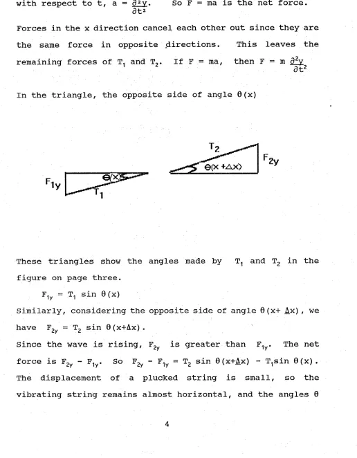
In the triangle, the opposite side of angle 0(x)

T

2y

e(x +Ax>

X

These triangles show the angles made by

T^ and Tg in the

figure on page three.

Fly =

sin 6(x)

Similarly, considering the opposite side of angle 0(x+ Ax), we

have Fjy = Tj sin 0(x+Ax).

since the wave is rising, Fgy is greater than F^y. The net

force is Fjy - F^y. So F^y - F^y = Tj sin 0(x+Ax) - T^sin 0(x).

The displacement of a plucked string is small, so the

are quite small. When the 0 is very small, the tangent of 0

is approximately equal to the sine of 0. (Estimate from the

Maclaurin series)

So Fjy - F^y = '^2

+Ax) -

sin 0(x)

« Tj tan 0(x+Ax) -

tan 0(x)

But

= Tj, since the tension in the string is the same at

as it is for Tj. Therefore;

Fjy - F^y = T(tan 0(x+Ax) - tan0(x)).

Recall that tan 0(x) is the slope of the tangent lines at x

and x+Ax, or the partial derivative dv ■ 3x

So the net force is

- F^^ = Tf dv

-

[ dx dx)

at x+ Ax at X

But the net force is also F=ma, which is m d^v :

■ ■ . at2 ■ , therefore

- F^ ^ m d^,

2y

which implies

m d^v « Tf dv

-

dv )

3t2 I 3x 5x J

at x+Ax at x

Define u to equal the linear mass density, u = m . where m 1

is the mass of the whole string, and 1 is the length of the

string. So mass of a small piece of string is equal to u(Ax), where (Ax) is the length of a small piece of the string.

Therefore

u(Ax)d£y_ » Tf dv

-

dv 1

8t2 I dx dx J

at x+Ax at x

So d^v «Tf dv - dv 1

3t2 ul 5x dx )

at x+Ax at x

(4x)

Observe that in the limit we have the x derivative of dy.

dx

since Lim ffx+Ax) - ffx) is the derivative of the function

A-»o Ax

f=dv. which is the second partial of y with respect to x.

dx

We therefore have the wave equation where T/u is a positive

constant

d^v = T V. 8t2 u 5x2

We have just derived the wave equation using physical

properties. The wave equation has a constant T/u, which we

constant T/u becomes c^, where c is the speed of the wave. To

prove T/u = c^, we need some definitions .

Definition: The frequency f, is equal to the number of

vibrations per second, f = vib , where the units of the

sec

frequency are measured in hertz, Hz. The period P, is the

number of seconds per vibration, or P = 1 . The wave

f

length X is the length of one complete cycle of the wave.

I

A = wavelength

The speed of the wave is the distance the wave travels divided

by the time traveled.

Therefore, the wave speed c, is distance = X = X

time P 1

Suppose we have a traveling wave moving along the x-axis,

and at t = 0, the peak of the wave, f(x) is at x = 0. We

can describe the pulse at this mCment in time as the

displacement y as a function of position x.

y-axis

n

II

x-axfs

V,

;;:x=

We need a function that gives the same shape as but

moved to the right. At a later arbitrary time t, the of

the wave can be pictured as the following;

y-axis

"VM

x-axis

x=0

The pulse is moving at speed c. Therefore it has moved a

distance of ct. A function that represents this displacement with time t is f(x - ct). So whatever the shape of the wave f(x) describes, f(x - ct) describes the same shape but at a later time t. The peak of the wave of f(x) is at x = 0,

whereas the peak of the wave of f(x - ct) is at x = ct. An

example of such a wave at t = 0 is given by the equation

y = y^cos(27rx/A) where y is the vertical displacement

from the point of equilibrium, the maximum displacement or

amplitude is y^, and X is the wavelength.

x-axis

= wavelength

We need to describe the wave's position at time t. Replace x

by X - ct.

y = y^cos27r(x - ct)

y = y^jCos(27rx/A - 2nctlX)

c = fX implies = f

y = y^jCos(27rx/A - 27rft)

Let k = {2tt/X), where k equals the wave number. The

wave number describes the number of radians of a wave

Let (i) = 27rf.

Therefore we have y = y^jCosCkx - et) as a solution to our

equation, = T d^v

5t2 u 3x2

liote;

Y = yQCOs(kx + wt) is also a sblution; it is a wave

moving to the left along the x-axis. To relate the constant

T/u in the wave equation to the constants in a periodic

solution we substitute the cosine solution into the wave

equation: d^v = -yj,w2cos(kx - wt), d^v = -y k^cosCkx -ot)

3t2 3x2

then

32 V

T = 3t2

= -v_.e2cosfkx - <atV

u

32V

-yQk2cos(kx - (ot)

3x2■ ■■

T = 0)2 , But a - 2nf and k = 2n . so

u k2 X

XZjitXL = 47r2f2 __Ad_ = f2A,2 = c2.

u (2it/A.)2 4772

So the equation for the string that vibrates near the

point of equilibrium is 32y - c^d^v . where c =

3t2 3x2 sj u

If y = $(x,t) is a periodic solution then we have shown that

c is the wave speed. Recall that T is the tension in the

string and u is the linear mass density. Observe that as the

string becomes longer the wave speed slows, and as T grows the

string is tightened and the speed of the wave is faster.

§1.2 SOLUTIONS Tb THE

We now want to look at what types of functions satisfy

the wave equation. We will show equations of the form

y = f(x ± ct) are solutions to the wave equation/ where f is

any function of one variable. [12]

Since f is a function of

one variable it's derivitives can be defined as f and f'.

Let f, and fg be arbitrary functions.

Show that

y = f^(x - ct) is a solution to the wave

equation,

= c^d^v .

5t2 8x2

Find the first and second partials of y with respect to t and

">■* 8y = -cf. • (x - ct) .

82V = c2 f ' ' (x - ct)

and

8y = f/ (X ­

8x ■

82 V = f ' • 8x2

So ■ ■ 82 V = c2

, 3t2 8x2,/' ■

Therefore, y = f^ (x - ct) is a solution to the wave equation.

Show that

y = fgCx + ct) is a solution to the wave

8v = cfp' (X + ct)

d^v =c2f-''(x + ct)

at2

and

8v = fp*(x + ct)

d^v = fp"(X + ct).

3x2

Again, d^v - c^ 32y .

3t2 3x2

Therefore, y = fjCx + ct) is a solution to the wave eguationv

Because the wave equation is a linear equation, any linear

combination y = A f^(x - ct) + B fgCx + ct) is also a solution

to the wave equation. Sine and cosine functions satisfy the

wave equation, but functions such as exponentials will also

satisfy the equation [2].

Show the wave equation has an exponential solution.

Let y = e"*e®*.

Then

3v = 3t

32V = (22 e^^e®^

3t2

3v = Be"^e®*

3x

32V = 62e«*e®*. 3x2

Substitute the second partials into the wave equation.

= c262

6 = ±a , So y = "■Vc-­

= gat+ax/c

and

72=

Therefore y:, and yj are also solutions to the wave equation

but not physically realistic. There are other solutions to

the equation.

To find them all we need Fourier Analysis,

which is beyond the scope of this paper.

§1.3 SOLUTIONS OF THE FORM $ = X(x)T(t)

If we have a linear second order ordinary differential

equation with constant coefficients, we can easily find the

general solution.

If the solution a partial differential

equation can be represented as a product of independent

functions X(x)T(t), we can separate the functions and solve by

using general solutions from O.D.E. Assume that t(x,t) is a

solution of the form $ = X(x)T(t), where X is a function of

X, and T is a function of t.

= X'(x)T(t)

3$ = X(x)T'(t)

,;dx

■ ■ ■

dt

_ai§_ = X''(x)T(t)

_dli_ = X(x)T''(t)

ax2 at2

Plug the second partials into the wave equation.

XV'(x)T(t)= 1 X(X)T'•(t)

■ yVV C2

Divide both sides by § = X(x)T(t).

X''rx^Tft) = 1 Xfx^T''(t)

X^(^^

c2 X(x)T(t)

X"fx) = 1 T''ftV X(x) c2 T(t)

The left hand side is a function of x only, and the right hand

side is a function of t only. The on^^^^^

can happen is

if both sides are equal to a constants

This constant is

called the separation constant. Let the separation constant

be a negative number.

We use -^m— instead of m^ to insure

periodic solutions, and so that later boundary conditions will

be satisfied.

X''fx^ = 1 T''ft) = -in2 X(x) c2 T(t)

So X«'Cx^ = -m^ and 1 '(t) =

X(x) c2 T(t)

X''(X) = -in2X(x) and T''(t) = -m^c^TCt)

Both equations are second order ordinary differential

equations. Two independent solutions to X''(x) + in2X(x) = 0

are

=

sin(mx) and

^ cos(mx). Two independent solutions

to T''(t) + m2e2T(t) = 0 are §3 = sin(met) and

= cos(mct).

([2], page 114). Hence, setting X(x) = A sin(mx) + B cos(mx)

and T(t) = G sin(mct) + D cos(mct) a solution for the partial

differential equation is

§(x,t)=[A sin(mx) + B cos(mX)][C sin(mct) + D cos(mct)]

In chapter one we saw the derivation of the wave equation

using physical properties. Solutions that satisfy the wave

equation were calculated, and it was shown that arbitrary

functions f^, f2 of the form

y - f^ fx - ct) + f2(x + ct)

satisfy the wave equation.

In section three, it was

demonstrated that $(x,t) has solutions of the form

$ = X(x)T(t),

§2.1 SOLVE THE WAVE EQUATION FOR THE STRING FIXED AT BOTH ENDS

In chapter two, two cases for the vibrating string will

be solved. The first case is where the string is fixed at

both ends like that of a guitar or violin string. The second

case is that of a string fixed at one end and the other end is

allowed to travel up or down the line x = x^.

We need to

formulate boundary conditions that describe the physical

properties of the string.

These boundary conditions will

enable us to determine the constants A,B,C,D in the solution

§(x,t)=[A sin(mx) + B cos(mx)][C sin(mct) + D cos(mct)].

5-axis i(x.l)

x-axis x=o

This graph shows the position of the vibrating string at time

t, with the ends fixed at x=0 and x=L, with vertical axis

y - § arid horizontal axis x.

J -axis

Itx.t)

t2

13

x-axis x=o

This illustration shows the string fixed at both ends with

different values of f at x^ for different times t..

t-axis

I M I'U I I 1.^

11

This illustration shows the string's position at x^^ for

various times t..

Having the string fixed at both ends imposes boundary

conditions on the wave equation.

The boundary conditions are as follows;

B.C #1 §(0,t)=0 (This implies X(0)=0 V t e T)

B.C.#2 $(L,t)=0 (This implies X(L)=0 V t e T)

B.C.#3 $(x,0)=0 (This implies T(0)=0 V x e X)

B.C.#4

3$(x^.0)=v (For some Xjj e X, x^ =v, when t-0, where

point x^)

A node is a place in which the function is always zero.

Boundary conditions number one'states the function has a node,

at X =0, which implies the string is at rest. Boundary

condition number two states the length of the string is L,

and at thisi point is there is another node. Boundary condition number three states that at time zero the string is

at rest, and boundary condition number four states the

velocity of the string at a fixed point on the string at time

zero is a constant v.

Assume that §(x,t) is a solution of the form

# = X(x)T(t).

In section 1.3 we found a periodic solution

#(x,t) = [A sin(mx) + B cos(mx)][D sin(cmt) + E cos(cmt)].

Test the boundary conditions.

B.C. #1 §(0,t)=0 implies

[A sin(O) + B cos(0)][D sin(cmt) + E cos(cmt)] =0

B [D sin(cmt) + E cos(cmt)] = 0

Either B = 0 or [D sin(cmt) + E cos(cmt)] = 0 V t.

If [D sin(cmt) + E cos(cmt)] = 0 then D sin(cmt) = E cos(cmt),

which is a contradiction since the sine and the cosine cannot

be proportional, so D = E - 0. But this is the trivial wave,

therefore in a nonzero solution, B - 0.

So §(x,t) = A sin(mx) [D sin(cmt) + E cos(cmt)],

B.C. #2 §(L,t) =0 implies

A sin(mL) [D sin(cmt) + E cos(cmt)] = 0

Either A sin(mL) = 0 or D sin(cmt) + E cos(Gmt) = 0 V t.

If D sin(cmt) + E cos(cmt) =0 then, we have the trivial

wave again, therefore A sin(mL) =0.

A sin(mL) = 0 implies mL = kTT, k e Z

Hence m = k7r. L

So $(x,t) = A sin(k7rx/L) D sin(ck7rt/L) + E cos(ck7rt/L).

B.C. #3 f(x,0) = 0 implies,

A sin(k7rx/L) D sin(O) + E cos(O) =0

A sin(k7rx/L) E =0, therefore E = 0.

So §(x,t) = A sin(k7rx/L) D sin(ck7rt/L)

Let AD = G,

$(x,t) = G sin(k7rx/L) sin(ck7rt/L)

B.C. #4

_aj&(x ,0) = V

at

Find the derivative of $(x,t) at (x^, 0):

a§ = (GkTTc/L) sin(7rkx^/L) cos(O) = v

(GkTTc/L) sin(7rkXQ/L) = v

G = vL

kTTC sinCTrkx^)

Therefore our solution under these boundary conditions is

$(x,t) = vL sinfTTkx/L) sinf7rkct/L)

kTTC sin(7rkx^)

Where V is velocity of the string at x^, L is the length of

the string, c is the wave speed, and k is an arbitrary

integer. We can rewrite the equation as

( vL sinf7rkx/L) sin(7rkct/L) V

dt21

kTTC sin(7rkx^),

J

=- fTTkcV^ VL sinfTrkx/LV sinf7rkct/Ll .

I L j

kTTc sin(7rkx^)

This has the form of an operator times a function, which

equals a constant times the same function. The solution $ is

an eigenfunction of the Laplacian L = d± with eigenvalue

-(7rk/L)2. The solution 4 is also an eigenfunction of the

operator 5i. with eigenvalue -(7rkc/L)2. The

3t2

eigenvalue is the negative of the square of the angular

frequency w, which is in radians per second. So w = Trkc/L. The regular frequency f, is in cycles per second, and there

are 27r radians per cycle. Therefore if we divide w by 2n we

get f = kc/2L. Hence the frequency that produces the sound

that is emitted from a vibrating string fixed at both ends is

kc/2L, where

k = 1,2,... As k runs through the integers an infinite number

of frequencies are produced. What we hear is combinations of

these frequencies.

Certain combinations are perceived as

noise, whereas other combinations are pleasant sounding and as music. So different frequencies produce different sounds, and

the higher the frequency the higher the pitch. This implies

by our kc/2L, that the higher the pitch the faster the wave

speed. Notice as L (the length of the string) gets larger,

the pitch will be lower.

Sound that we perceive as musical notes have their

frequencies in the following ratio form [13],

C D E F G A B G'

3 5 15 2

8 4 3 2 3 8

9 5 4

For example the note E, has a frequency 5/4 times that of the

note C, and F has a frequency 4/3 times that of C. The note

C' has twice the frequency of C.

Consider one octave on a piano.

D G A B

fl

9fi 5f^

4f, 3f^ 5f^

15f, 2f,

. 8 .;/■ /4..., 3 ■ : ■ 2 ■ ■ 3 V ' 8

There is no absolute standard of pitch.

The definition of

middle C, for example, has changed over the decades [13], but

the ratios defining a scale are determined by the wave

equation, as we shall see. Currently it is agreed that A has

a frequency of 440 hz. If the frequency of middle C = is

taken to be 264 hertz, then G is 396 hz, and C'=2f^ = 528 hz.

Also, as we go up an octave each of these ratios are in

the following form

Up one octave from f,,

D'=2(9f,)

E'=2(5f,)

F'=2(4f,)

8 . 4 ■ '•;- 3 ■ ,

D'•=22(9f,)

E''=22(5f,)

F''=22(4f,)

8 V-::/. '''

:

4

^

■ ■

3

-

'

D"•=2'(9f;)

E'"=2^(5fi)

F'"=22(4f,)

Consider the frequencies that appear in the solution of

the wave equation. The corresponding notes are

=

Ifi - (the fundamental frequency)

Cj = 2f^ = (the first harmonic or overtone)

Gj

— 2(3/2)f^ = 3f^ (the second harmonic or overtone)

• C3 = 22f^ = 4f,

■

;

E3 = 22(5/4)f^ = 5fi

G3 = 22(3/2)f, = 6f,

. B3'' = 22(7/4)f, = 7f,

= 8f,

Recall f = kc/2L where k = 1,2,3.... This is what just came

out of our calculations. When a guitar string is plucked,

the sound is a combination of these notes. The fundamental

tone is the most prominent.

§2.2 SOLVE THE WAVE EQUATION FOR A STRING FIXED AT ONE END

We will now solve the wave equation for the string fixed

at one end, and allowed to move up and down the line $(x) =x^j.

()- axis

x-axis

x=o

X = L

Boundary Conditions,

B.C. #1 $(0,t) =0 (This implies X(0)=0 V t e T)

B.C. #2 ^(L,t)=0 (This implies that V t e T the slope dx of the string is zero at x = L)

B.C. #3 f(x,0)=0 (This implies that function is zero

at t=0)

B.C. #4

(x^.0)=v (This implies that the piece of the

3t string at x has velocity v at t=0)

Assume the solution to be of the form §(x,t)=X(x)T(t).

From previous work in section 1.3, a solution is

$(x,t)=[A sin(mx) + B cos(mx)][C sin(mct) + D cos(mct)].

Test the boundary conditions.

B.C. #1 $(0,t) = 0 implies

[A sin(O) + B cos(O)][C sin(mct) + D cos(met)] = 0

so either [A sin(O) + B cos(O)] = 0 or

[C sin(mct) + D cos(mct)] = 0, contradiction unless

C = D = 0 which implies the trivial solution. The trivial

solution is a flat wave which is not very interesting,

therefore B - 0. Our solution is

§(x,t)= A sin(mx) [C sin(met) + D cos(met)] B.C. #2 _dl_(L,t)=0 implies

dx

= Am sin(mL) (C sin(met) + D cos(met)) = 0,

5x

So either Am sin(mL) = 0 or C sin(met) + D cos(met) = 0, as

before contradiction unless C = D = 0, which is the trivial

wave, so Am sin(mL) = 0. Therefore m = 7rk/L where k e Z.

f(x,t) = ATTk/L sin(7rkx/L) (C sin(7rkct/L) + D cos(wkct/L))

B.C. #3 §(x,0)=0 implies

Avrk/L sin(7rkx/L) (C sin(O) + D cos(O)) =0. So D = p, and our

solution is

$(x,t) = ATTk/L sin(7rkx/L) C sin(7rkct/L). Let ACTrk/L = F;

then $(x,t) = F sin(7rkx/L) sin(7rkct/L)

B.C. #4

^ (x„,0) = V implies

^(x ,0) = F sin(7rkx /L) 7rkc/L cos(O) - v

at

F sin(7rkx^/L) vrkc/L = v

which implies

F = vL/(7rkc sin(7rkx^/L))

So our solution for a string fixed at one end is

$(x,t)= vL sin(7rkx/L) sinfTrkct/P

TTkc sin(7rkx^/L)

As before our eigenvalue is -(Trkc/L)^, and our frequency is

kc/2L.

In chapter two we have seen the solutions for the string

fixed at both ends, and for the string fixed at one end. From

the particular solution an eigenvalue was found which was the

negative of the square of the angular frequency. From the

angular frequency the regular frequency was calculated by

dividing by 27r. The frequency could then be correlated to

notes on a musical scale which we perceive as pleasant sound.

§3.1 THE WAVE EQUATION IN IN CYLINDRICAL COORDINATES

In the previous sections we have worked with the wave

equation involving just x and t. To solve the wave equation

on the cylinder, we need the wave equation in three

dimensions,

3^$ + 3^$ + 3^$ = 1 3^$» Since we will be

3X2 3y2 3Z2 C23t2

solving the wave equation for the cylinder, it will be easier

to use cylindrical coordinates. We will now change the three dimensional wave equation from rectangular coordinates into

cylindrical coordinates. We will then solve the equation for

the cylinder. Change (x,y,z) to (r,0,z), where r^ = x^ + y2

and 6 - tan'^y/x) [4]. From the above information we can

derive the following partials.

3r = COS0 30 = -lsin0

3x 3x r

We will assume that $ is C^; that is all second partial exist

and are continuous. Therefore mixed partials are equal.

3$ — 3$ 3r + 3j^ 3j9 3x 3r 3x 30 3x

3j& = d§ 3r + 3^ 3^

3y

3r 3y

30 3y

3$ = 3$ 3z 3z

We want the second partial of §:

32$ = 3 f3^ 3r1 + d_{

30)

3x2 3xl0r 3xJ 3xl0r dxj

=d (d§]dr + d f dr]d§ + d 13$)36 + d f38V 3$

3xl3rJ dx

dxlSxj dr

dxldQl^x

dx^^

36

3fi cos6 + 3 (cos6)

+ 3f,^"1 sin6l + 3 f- 1 sin6l

dx

dx

dr

dx I r

1

3x1 r

J

where f, =^ and

f, = 3#.

■ ■ V ■■ 36r ■

=

3f, cos6 + 3fp f- 1 sin 61

(equation 1)

dx dx [ r

3 fI = 3 f3$1 3r + 3 f3$1 36

dx drldr) dx 36l3rJ dx

d fI = d^§ cos6 - 1 sin6 3^$

dx dr^ r 363r

3_fp = 3 f3$1 3r + 3 f3$1 36

dx 3rl36J dx 36136j 3x;

3_fp = 3^$ cos6 - 1 sin6 31$

dx 3r36 r 36^

Using equation 1, substitute

3 f, ahd 3 f,

V dx ' ■3x

3^$ = cos6(cos6 3^$ - lsin6 3l$ 1

3x2 I 3r2 r 363rJ

- 1 sin6 f3^$ cos6 - 1 sin6 3$ll

r

I3r36

r

362j

cos6 3_fcos6 3$ - 1 sin6 3$1

3rI

3r

r:

36j

1 sin6 i3fcos6 3^ - 1 sin6 3$1

t

36^^^^^^^

3r

r

36j

= COS0 fd£$ cos6 + 1 sin0 3§ - 1 sin0 di \

Id?

, rf;

30 r

0r00j

1 sin0 fd^l_ c6s0 - sin0 3$

1 cos0 3$ - 1 sin0 3$T

r l303r 3r r 30 r 30j

cos^0 3^$ + 1 sin0cos0 ^ - 1 sin0cos0 3i#_

3r^ 30 r 3r30

1 sln0cos0 3^$ + 1. sin^0 3$ -f 1 sin0cos0 3$

r

303r

r

3r

?

30

+ 1 sin^0 3f.

30

Therefore

3^$ = COS20 3^$ +2 sin0cos0 3$ - 2 sin0cos0

3x2 3r2 r^ 30 r 3r30

+ 1 sin20 ^ + 1 sin^0 d^§.

^ .

3r

r2

30^

A similar derivation shows that

32$ = sin20 32$ t 2 sin0cos0 32$

'■2 ' ...v ■ ,3r2 dddr ■

- 2 sin0cos0 3j|, + 1 COS20 3$ + i cos20 32$, ■' , ,/r2:'V ' - dd ■ . ;'r;,'-'> dr r^ 36^

Plug the partial derivatives into the wave equation

1 324 = 32# 4- 32# + 32$ ■„

C2 3t2 3x2 ^ 0y2 022

1 32$ = COS2 0 32$ + 2 sin0cos0 3$

c2 3t2 3r2 r^ 30

2 sin0cos0 3i$_ + 1 sin2 0 3ji + 1

r 3r30 r 3r r2 30^

+ sin20 02$ +2 sin0cos0 02$ - 2 sin0cos0 0$

0r2 r 000r r2 00

+ i COS20 0$^ + i COS20 02$ + 02$

r 0r r2 002 0z2

1, 02$ = cbs20 02$ + sin20 02$

C20t2 0r2 0r2

+ 02$

+ 1 sin^0 0^$ + 1 COS20 02$

r2 00^ 00^ 0z2

1 9^$

= 02$ (cos^0 + sin^0) + 1 ^$ (cos^0 + sin^0)

302

G20t2 0r

+ 1 ^ (cos^0 + sin^0) + 0^$

r 0r 0z2

1 02$ = 02$ + 1 ^$

+ 1 M + 0^$

C20t2 0r2 00^ r 0r 0z2

02$ + 1

Note: 1 0 (r 0$1

0$ + r 0^$

r 0rl 0rj 0r 0^r 0r2 r 0r

Therefore the wave equation in cylindrical coordinates is

1 0_(r 0$1 + 1 ^$

+ 0^$ = 1 0^$

r 0rl 0rj

r^ 00^

02^

c20t2

§3v2 S0l^E THE WAVE EQUATION

The case of the cylinder can be generalized from the case

of the vibratihg string. The string gscillates up an

in

a plane until eventually coming to rest at the point of

equilibrium. The restoring forces pull the string toward the

point of equilibrium.

Likewise, the cylinder vibrates

radially, as the restoring forces pull the wave back toward

the point of equilibrium which is the surface of the cylinder. The direction of vibration can be thought of as a normal

vector to the surface of the cylinder. We will assume that

both ends of the cylinder are clamped, which is analogous to

the string fixed at both ends.

Z-UIS

Z-H

T-illS

I-illS

In cylindrical coordinates the wave equation is

1 d_(r5§J + 1 $ + 8^$ = 3. 8^$

r 8rl 8rJ dz^ c^ dt^

The radius of the cylinder is a constant R and so all

derivatives with respect to r are zero; therefore, the first

term is zero. So our wave equation becomes.

802

1 3>* +di§ = 1 _d±i, where $ = §(0,z,t) a function

R2 302 3z2 c2 3t2

of three variables.

Boundary conditions;

1) f(0,z,O)=O (Implies the cylinder is initially at rest

V 0,z)

2) §(0,O,t)=O (Implies a node at the bottom of the cylinder

V 0,t)

3) $(0,H,t)=O (Implies a node at the top of the cylinder

V 0,t)

4) M = (eo,z„,0) = V

Boundary condition number one implies at time equal zero, the system is at rest. Conditions number two and three state that

there is a node at every point along the bottom of the

cylinder, and at every point along the top of the cylinder.

Recall the nodes are places on the wave where the function is

identically zero. Condition number four implies that at time

zero, the velbcity at a specific point on the cylinder 0^, z^,

is V.

Assume $ - $(0,z,t)=0(0)Z(z)T(t)

82$ = 0«'(0)Z(z)T(t)

82$ = 0(0)Z'•(z)T(t) ,

8z2

82$ = 0(0)Z(z)T''(t)

8t2

Substitute the partial derivatives into wave equation

1 0'•(0)Z(z)T(t)+0(0)Z"(z)T(t) = 1 0(0)Z(z)T'•(t)

R2 c2

1 0"(0)Z(z)T(t)+0(0)Z"(z) = 1 0(e)Z(z)TLLltl

R2 C2 T(t)

1 0''(0) + Z''fz^ =1 T''rt)

R2 0(0) Z(z) c2 T(t)

The left hand side is a function of 0 and Z, and the right

hand side is a function of T. Both sides are independent, so

they must equal a constant. Let the constant equal -m^.

1 T''ft) = -m2 implies T*'(t) + m^c^TCt) =0

c2 T(t)

T(t) = A sin(met) + B cos(mct)

Test boundary conditions #1.

Notice this is work from the one dimensional case.

B.C. #1 §(0,z,O) =0

T(O)0(0)Z(z) =0

T(0) = A sin(O) +B cos(O) which implies B=0.

so T(t) == A sin(mct)

Separate the left hand side.

1 0''f0) + Z''f z) = -m2 R2 0(0) Z(z)

1 0''f0) = -m2 - Z''(z)

R2 0(0) Z(z)

Again, both sides must be constant. Let the constant be -n2. 1 0"f0) = -n2 implies 0"(0) + n2R20(0) = o

R2 0(0)

So 0(0) = C sin(nR0) + D cos(nR0)

Z''fz) + m2 = -n2 implies

Z(z)

Z' * (z) + (m2 - n2)Z(z) =0 has a solution of the form

Z(z) = E sin(Vm2 - n2 z) + F cos(Vm2 ^ n2 z)

B.C. #2 §(6,0,t) =0

Z(0) = E sin(O) + F cos(O) = 0 implies F = 0

Z(z) = E sin(Vm2 - z)

B.C. # 3 $(0,H,t) = 0

Z(H) = E sin(Vm2 - n2 H) = 0

Let (Vm2 -n2)H = p7r 3peZ

Vm2 - n2 = gTT

H

ra = (p27r2 - /H

So Z(z) = E sin(p7rz/H)

Now T(t) = A sin(ct[p27r2 ­

0(0) = C sin(nR0) + D cos(nR0)

Z(z) = E sin(p7rz/H)

§ = (C sin(nR0) + D cos(nR0))

• E sin(p7rz/H)' A sin(ct[p27r2­

For solutions to be defined on the cylinder, nR

where j e Z. So n = j/R

Let G = EA.

$ = G(C sin(j0) + D c6s(j0))

• sin(p7rz/H) sin(ct[p27r2 - j /R2]

B.C. #4

dA (0^,z^,O) = V

at

a$ = G(C sin(j0 ) + D cos(j0 ))

at

•sin(p7rz^/H)• cos(O)' c(p^iT^ -

=v

V = Gc/H (C sin(j0jj) + D cos(j0jj))

• sin(p7rZjj/H)• (p^yr^ ­

G = V

abed

a = (p27r2 - j2H2/R2)''''2/H

b= sin(pttz^j/H)

d= C sin(j0jj) + D cos(j0g).

Therefore the solution, subject to these boundary conditions

is

$ = V rc sinfi0) + D cosM0)1 sinfP7rz/H) sinfact)

abed

Using a trig identity, let

C sin(j0) + D cos(j0) = VC2 + D2 sin(j0 - $) where tan$ = D/C,

and

C sin(j0Q) + D cos(j0^j) = VC2 + D2 sin(j0Q - i)

Therefore

4 = V fVC2 + D2)sin(i0/ - g) sin(P7rz/H^ sinfact)

a c b (VC2 + D)sin(j0^ - $)

§ — V sinM0 - E) sinfPTTz/H) sinfact^ .

cb sin(j0^ - $)

Therefore replacing a and b our solution becomes

$ = vH sinM0 -

sinfPTTz/H) sin(ct(02712- i2^2/Rz)Y^/h)

♦

c sin(p7rz^/H) sin(j0|j - i) (p27r2-j2H2/R2)

Where R and H are the radius and the height of the cylinder

respectively, c is the wave speed, v is the initial velocity

of a point on the cylinder of the wave, and p and j are

integers. The solution f is an eigenfunction of the Laplacian

and also an eigenfunction of with eigenvalue

■ -■ ■ ■ dt^

-c2 ^ /R^)• The frequency can be calculated as before.

■ ■H2

It can be seen from the particular solution, that the radius

and height of the cylinder have an effect on the sound. If

the cylinder is shortened the pitch will become higher, and if

the radius is widened the pitch will become lower.

In conclusion, a connection between sound and mathematics

is the eigenvalue of a particular solution for a second order

partial differential equation. Once the eigenvalue is khown,

the angular frequency and then the regular frequency can be

calculated for the wave. The frequency then corresponds to a

note from the musical scale, and we perceive these frequencies

as music. If we were to observe the frequency on an

oscilloscope, which breaks down the frequency by components,

we would see the different waves which makes up the harmonics.

REFERENCES

[1]

■

Bleistein, nV, Mathematical Methods for Wave Phenomena,

Academic Press, 1984

[2] Boyce, W., & DiPrima, R., Elementary Differential

Equations, Wiley, 1986

[3] Braun, M., Differential Equations and Their

Applications, Springer-Verlang, 1975

[4] Chisholm, J.SrMathematical Methods in Phi^sics, W.B.

Saunders Co. 1966

[5] Coulson; C.A'7' Waves,j ^

[6] Crhndall, I., Theory of vibrating systems and sound. Van

[7] Feynman, R., The Feyriman Lectures on Physics, Addison-^

"V'-'

■; ■ ■ wesley,. \i963 ^/'y' : :■ ■

[8] Friedlander, F.G., The Wave Equation on a curved

[9]

Kane, J., Physics., Wiley, 1978

[10] Kibble, T.W.B.: Classical Mechanics, McGraw Hill, 1973

[11] Lindsay, R., Physical Mechanics, Van nostrand Co., 1933

[12] Pain, H.J.: Physics of Vibrations and Waves, Wiley &

[13] Rayleigh, J.W.S., The Theory of Sound, Macmillan Co.,

[14] Strang, G^, intirciductidn to Applied Mathematics,

[15] Weinberger, H.F., Partial Differential Equations,

Blaisdell, 1965

[16] Wolfson, Richard: Physics, Little Brown & Co., 1987