http://www.sciencepublishinggroup.com/j/sjams doi: 10.11648/j.sjams.20180603.14
ISSN: 2376-9491 (Print); ISSN: 2376-9513 (Online)
Determination of Optimal Public Debt Ceiling for Kenya
Using Stochastic Control
Millicent Kithinji, Lucy Muthoni
Strathmore Institute of Mathematical Sciences, Strathmore University, Nairobi, Kenya
Email address:
To cite this article:
Millicent Kithinji, Lucy Muthoni. Determination of Optimal Public Debt Ceiling for Kenya Using Stochastic Control. Science Journal of Applied Mathematics and Statistics. Vol. 6, No. 3, 2018, pp. 90-98. doi: 10.11648/j.sjams.20180603.14
Received: May 13, 2018; Accepted: June 19, 2018; Published: July 23, 2018
Abstract:
Public debt is a key economic variable. It is the totality of public and publicly guaranteed debt owed by any level of government to either citizens or foreigners or both. Due to recent debt crises in countries such as Portugal, Italy, Ireland, Greece and Spain, debt control has become a key important fiscal policy of every government. In this study, we applied a Public debt ceiling explicit formula to find out the optimal public debt ceiling for Kenya [3]. We made modification to subjective variables in the explicit formula and used the formula to find the optimal public debt ceiling for Kenya. We illustrate that it is prudent for that government to use a fiscal policy that maintains the debt ratio under an optimal debt ceiling.Keywords:
Stochastic Optimal Control, Public Debt, Debt Ceiling, Hamilton-Jacobi-Bellman Equation, Value Function, Control Process1. Introduction
1.1. Background of the Study
Public debt is a key economic variable. It is the totality of public and publicly guaranteed debt owed by any level of government to either citizens or foreigners or both. Controlling the debt/GDP ratio and keeping it below the debt ceiling is essential to both developing and developed countries. Various researchers have used different approaches to demonstrate the demerits of a high public debt to the economy. For instance, an increase in the volume of public debt can have some undesirable outcomes in the economy; such as inflation, shrinking of private investment, lowering of future growth and wages, high finance cost and repayment burden.
Due to undesirable outcomes of high debt levels, countries and regional trading blocs have developed fiscal policies to tame their respective debt/GDP ratio to a given level. For instance, in East African Community (EAC), the debt ceiling is set at 50% of GDP for all member states. For instance, as at June 2016, Kenya's gross public debt stood at 48.3% of gross public debt percent of GDP in present value terms [4]. In December 2014, the Kenyan Legislature raised the maximum amount the national treasury can borrow from
Ksh. 1.2 trillion to KSh. 2.5 trillion. Hence, the problem we study is that of determining how much debt a country can accumulate without a negative impact on economic growth.
Our aim is to find out the optimal public debt ceiling for Kenya. By optimal public debt ceiling, we mean; the minimum limit of debt/GDP ratio at which the government should start implementing debt control measures. By control measures, we mean that it is possible for the government to decrease the debt/GDP ratio through fiscal measures such as increasing taxes or decreasing expenditure. This implies that, the government should put fiscal adjustments measures in place when the debt ratio is above the optimal debt ceiling.
The study on optimal debt ceiling using stochastic control has not been studied before in Kenya. Hence, the study will contribute to the literature of public debt.
In this study, we adopted a theoretical model proposed by [3]. In the model, they developed an explicit formula for determining optimal public debt ceiling for a given country. We chose to use their model because it is country- specific since it uses macroeconomic variables for each country.
the corresponding value function.
Due to recent debt crises in countries such as Portugal, Italy, Ireland, Greece and Spain, debt control has become a key fiscal policy of every government. Due to the need for debt control, different regional trading blocs such as East African Community, European Economic community, and various countries have set their maximum debt ratio to a given percentage. This implies that, each member country should maintain their debt ratio below the given debt ratio ceiling. These debt control measures have been put in place in recognition that governments all over the world borrow. This is because the government revenue raised through taxes and fees is not enough to meet the entire government expenditure leading to a budget deficit. Hence, borrowing is inevitable. However, high public debt has undesirable effect on the economy and therefore should be controlled.
Despite the existing debt ceilings in various jurisdictions, the debt ceilings have not been previously developed using a theoretical framework. Hence, the recent framework for developing an Optimal debt Ceiling Formula is is a ground breaking research in stochastic control methods for public debt management [3]. Our contribution to Optimal debt ceiling literature is application of Stochastic control to determine the optimal debt ceiling for Kenya with an aim of advising the public debt policy.
1.2. Objectives of the Study
The main objective of this study is to determine the optimal debt ceiling for Kenya using stochastic control approach. We seek to address the question; What is the optimal debt ceiling for Kenya ?
Specific Objective
1. Determine the the optimal Public debt ceiling for Kenya.
2. Determine the Value function (the minimum cost incurred by the government at a given debt ratio when all admissible controls are considered.
2. Literature Review
Stochastic optimal control was first introduced to economics and finance literature by Merton in 1971 who studied the optimal portfolio selection problem in continuous time. In his framework, Merton modeled the portfolio as a controlled stochastic process and found the optimal investment strategy that maximizes a given objective. He used PDEs known as Hamilton-Jacobi-Bellman equations to obtain more precise solutions in continuous time portfolio optimization [6].
Since then, stochastic optimal control has been used in studies that seek to determine the optimal debt ratio. For instance, a formula for optimal public debt ratio for public and private sectors using Bellman’s techniques has been derived. The model considered capital productivity, return on asset, interest rate, and regime switch on the market where the goal of the controller was to maximize the utility of wealth at Maturity by selecting an the optimal debt ratio [7].
In Stochastic control problems, the behavior of a dynamical stochastic process is influenced to obtain a given goal. The notion of control means that behavior of a dynamic system is influenced with an aim of obtaining a given goal. If the aim is optimizing a given objective function that relies on the control inputs into a system, then we have an optimal control problem. The fundamental components of a Stochastic Control problem are:
1. State Process, X. This process defines the nature of the physical system of interest. It captures the minimal necessary information needed to describe the problem. Typically, the process is influenced by the control. Usually, its time dynamics is prescribed through an ordinary or stochastic differential equation. The progression of the state process is influenced by a control.
2. Control Process, Z. This is a stochastic process, selected by the "agent" to influence the state of the system.
3. Admissible Control, . These are controls that meets admissibility conditions. The conditions either be technical or physical, for instance, continuity or smoothness conditions, and, budget constraints.
4. Objective Function. This is the function to be maximized (or minimized). The objective function is usually denoted as J(x, Z). It represents the expected total cost of the system when the control process is implemented.
5. Value function, V. This function defines the value of the minimum cost or reward. It is usually denoted by V and is obtained by optimizing the cost or reward over all admissible controls for a given initial state. The aim of a Stochastic Control problem is to describe the value function and find a control whose cost or reward achieves the minimum value over all admissible controls. The major problem in optimal control is to find the minimizing control process [1, 2].
= ( ) = inf∈ ( ; . )
Most of the literature on the study of Stochastic control use dynamic programming or the Hamilton-Jacobi-Bellman (HJB) framework rather than stochastic maximum principles. The HJB is central to optimal control theory.
There are two principal approaches for solving the SOC problem namely, the Pontryagin's maximum principle and Bellman’s dynamic programming [8, 9]. Pontryagin's maximum principle asserts that any optimal control along with the optimal state trajectory will evaluate the Hamiltonian system. The HJB System consists of a collection of ad joint equations and the maximum conditions. Bellman's dynamic programming divides the dynamic optimization problem into simpler sub problems. Bellman's dynamic programming rides on the optimality principle and defines the relationships in a set of optimal control problems whose initial time and states are different via the HJB equation.
The two methods are similar in that it is possible to deduce the Hamilton system from the HJB equation, and vice versa [10].
recursive nature of the problem and defines the value function of the objective function, as a function of the state process for the SOC [7]. In our study, the dynamic programming equation (HJB) is a second order linear inhomogeneous second ordinary differential equation (rather than a PDE). This means that in the inaction region the value function depends only parametrically on the variable associated to the purely controlled state [11].
Our problem is focused on finding the optimal debt ceiling for Kenya. This is motivated by the rising surge in public debt that has received increased attention from policy makers, practitioners and scholars. Some policy makers have focused on the importance of reducing Public debt. For instance, discussions around optimal public debt and investment policy during the period post the global financial crisis have been carried out. Risk management has been outlined as a main reason for supporting Debt reduction. Government premiums may be increased if public debt is high in the event of a catastrophic event in which a government bailout is essential hence causing heavy government borrowing inevitable. This poses a sovereign risk and could lead to a shout out from the market. Therefore, a low debt today decreases a potential government crisis in the future [12].
Much of attention has been focused on understanding optimal debt strategy and structure of public debt [13]. However, little attention has been given to the study of debt ceiling. Debt ceiling is defined as the level of debt ratio at which fiscal adjustments are not necessary. As a result, if a country's debt ratio is above that level, it is prudent for the government to take intervention measures to regulate the debt. However, if the debt ratio is below the debt ceiling, the debt is under control hence no need for fiscal adjustments [3].
The existing literature on public debt management addresses the key issues, but has no theoretical framework to address debt control problem. Apparently, the existing Public debt ratio ceiling are determined by empirical and statistical analysis but without a backing of the theoretical framework. There are existing theoretical models that focus on public debt management [14, 13, 15, 16]. However, the models do not examine the public debt-ceiling problem.
A theoretical model for studying debt ceiling was introduced for the first time in the literature in 2016 [3]. The model was proposed to be used by any government to regulate its debt by fixing a ceiling on its debt ratio. In the model, the Debt ratio follow the dynamics of a geometric Brownian motion when the debt ratio is below the debt ceiling. This is consistent with the stochastic debt ratio dynamics as illustrated in various macroeconomic literature. An explicit debt ceiling formula was derived. The formula is used to derive an optimal debt ceiling for each country. This is because the economic parameters in the formula are specific to each country.
Further, the government debt reduction problem was modelled over an infinite time horizon as a singular stochastic control problem. In this model, it is prudent for
government to enforce a fiscal policy that maintains the debt/GDP ratio under an inflation dependent ceiling. However, the Markovian formulation of the singular control problem is fully two- dimensional [11]. We however, leave the multidimensional singular control approach for future research.
In our study, we apply the public debt ceiling explicit formula model with slight modifications in the parameters used in the formula [3]. For instance, instead of using the discount rate as used in the model we applied the risk- free rate which is the Central Bank Rate (CBR). CBR the lowest rate of interest the Central Bank of Kenya charges on loans to banks. Hence, to capture the autonomy of the Central bank in determining the lending rate we used the CBR rate.
3. Research Methodology
To determine the optimal level of Kenya’s debt ratio ceiling, was obtained by solving the value function for the HJB equation. The value function took a form of a second order linear nonhomogeneous constant coefficient ODE rather than a PDE. The solution to the ODE was obtained explicitly hence finding the optimal debt ceiling.
3.1. The Model
3.1.1. State Process
Let (Ω, ℱ, ℙ) be a probability space with filtration
ℱ = { , ∈ [0, ∞)} where ℱ is the flow of information over time. A levy process, W, on (Ω, ℱ, %) taking values in ℝ' is a d-dimensional ℱ Brownian motion if:
1. W is ℱ -adapted
2. ∀ 0 ≤ + ≤ , , − ,., the increments are independent of ℱ.,
3. ,/= 0, a.s.
4. ∀ 0 ≤ + ≤ , , − ,.~1(0, − +)
5. The sample paths of W are continuous with probability of one.
Let 2 = {2 , ∈ [0, ∞)} represent the state variable which is a country’s debt ratio defined as:
2 =345.. <5?=. :; 645'7; (3<6) > :?= 345.. 6789:; <=8 > :?= (1)
The state process, X, follows a Geometric Brownian motion.
2 = + A / B2.C+ + A / D2.C,.− (2)
Given that,
B = (E − F) ∈ ℝ and D ∈ (0, ∞) are constants, B is the drift of the process and D is the volatility, W is a Brownian motion, E ∈ [0, ∞) is the real interest rate on debt, F ∈ G the rate of economic growth [3].
3.1.2. Cost Function
The government wants to select the control Z ∈ (x) that minimizes the cost function J definedby:
( ; ) = JK[A /L MN ℎ(2 )C + A L
Where,
k ∈ (0, ∞) is the proportional (marginal) cost for reducing the debt, R ∈ (0, ∞) is the government's discount rate, and h is a cost function given by ℎ(S) = TSUV+ W which is assumed to be non-negative and convex. The function h represents the economic cost of having debt.
3.1.3. The Value Function
This function defines the value of the minimum cost or reward. It is usually denoted by V. It is obtained by optimizing the cost or reward over all admissible controls for a given initial state. The aim of a Stochastic Control problem is to describe the value function and find a control, ∗ whose cost or reward achieves the smallest value, ( ) = ( , ∗) over all admissible controls. i.e. For : (0, ∞) → ℝ, the value function of optimal stopping time is defined as:
( ) = inf∈ ( ; . )
3.1.4. The Control Process
This is a stochastic process, chosen by the agent i.e. the government to influence the state of the system. The control Z is given as = { , ∈ [0, ∞)}. The control process takes values in the control space, ℤ ⊂ ℝ].
An ℱ -adapted, non-negative, and non-decreasing control process ^, with /^= 0 and sample paths that are left continuous with right-limits, is said to be associated with the value function if the following three conditions are satisfied [3]:
1. 2 ^= + A / B2.^C+ + A / D2.^C,.− ^, ∀ ∈
[0, ∞), _ − . +.
2. 2 ^∈ `̅, ∀ ∈ (0, ∞), _ − . +. 3. A /Lb{cde∈ `}C ^= 0, _ − . +
3.1.5. Admissible Control
Controls which only meets certain admissibility criterion can be considered by the agent. The control, Z is adapted, non-negative, non-decreasing with left continuous with right limits (LCRL) sample paths i.e. : [0; 1)Ω ↦ [0, ∞), is a an admissible singular control, ( ∈ ) if ( ; ) ≤ ∞ .
( ) = is the set of all admissible controls. A control is admissible ( ∈ ( )) if there exists a unique solution to the state equation and if the transversality condition below
holds:
Conventionally, /= 0.
∀ ∈ ( ),
lim
j→LJK[ MNj2jUV= 0]
The transversality condition implies that in case there is a flexibility at maturity time, T, then the marginal benefit of taking advantage of that flexibility at the optimum must be zero.
3.1.6. Definition: Left Continuous with Right Limits, LCRL
A real valued stochastic process (2 ∈[/,j]) on (Ω, ℱ, %) is a LCRL stochastic process if ∀ ∈ [0, k]:
1. Left limit of the process as + approaches from the below (Left hand side) exists, i.e. lim.→ ,.l 2.= 2 M. Right limit of the process as s approaches t from the above (right hand side) exists, i.e.
lim.→ ,.l 2.= 2 m. 2. 2 M= 2
This means that, only the left continuity is needed hence allowing jumps. A continuous stochastic process therefore means that the process is LCRL.
3.2. Proposition
The value function is non-negative, increasing and convex. Furthermore, (0+) =nN
Let o: (0, ∞) → ℝ be a function in pU(0, ∞). We define the operator ℒ by
ℒo( ) =12 DU Uo( ) + B o( ) − Ro( ).
For a function s: (0; ∞) → ℝ in pU(0; ∞), consider the Hamilton-Jacobi-Bellman (HJB) equation
∀ > 0: min{ℒs( ) + ℎ( ), P − s( )} = 0 (4) We observe that a solution v of the HJB equation defines the regions ` = `^ and Σ = Σ^ by
` = `^: { ∈ (0, ∞): ℒs( ) + ℎ( ) = 0 C P − s( ) > 0} (5) ∑ = ∑ s = { ∈ (0, ∞): ℒs( ) + ℎ( ) ≥ 0 C P − s( ) = 0} (6) The regions ` and Σ form a partition of (0, ∞). That is, if
s solves the HJB equation, then ` ∪ Σ = (0, ∞) and ` ∩ Σ =
∅. It is possible to construct a control process associated with
s [3].
3.3. Solution to the HJB Equation
To obtain the optimal debt ceiling, we need to find the value function. The Hamilton-Jacobi-Bellman equation (4) in the continuation region ` = (0; {) implies
|
UDU Us( ) + B s( ) − Rs( ) = −T UV− W (7)
follows.
Let F = −T UV− W
2 = −_ UV+ }
2 = −2 _ UVM|
2 = −2 (2 − 1)_ UVMU
Replacing the derivatives in the ODE we obtain:
|
UDU U(−2 (2 − 1)_ UVMU)B (−2 _ UVM|) − R(−_ UV+ }) = −T UV− W (8)
Simplifying and equating like terms together in equation (8), we have:
{12 DU(−2 (2 − 1)_)} UV+ {B2 }} UV+ {R_} UV− R} = −T UV− W 1
2 DU(−2 (2 − 1)_ − 2B _ + R_ − T _ =R − DU (2 − 1) − 2BT
−R} = −W
} =WR
Hence,
2 =R − DU (2 − 1) − 2B +T WR
We now solve the complementary function2; . The corresponding homogeneous equation has the characteristic equation|UDU+ B − R = 0. To get the complementary function we find the roots of the equation.
1
2 DU+ B − R = 0
The two roots are given by:
2 =−{ + −√{2 U− 4
E1 =−B − €B2U+ 2DUR
E2 =−B + €B2U+ 2DUR
Hence, the solution to ODE equation is given by:
s( ) = p|exp(MŠm€ŠŒ‹‹mUŒ‹N)K+ pUexp(MŠM€ŠŒ‹‹mUŒ‹N)K+ T
R − DU (2 − 1) − 2B +WR
The HJB equation in the intervention region ∑ = [{, ∞) implies:
s( ) = s({) + P( − {) (9) The general solution of (8) and (9) is
s( ) = •Ž •|+ • •U+ T‘ UV+WR , if < {
P + “, if > {
Where,
B̅ = B −|UDU (10)
”|=MŠ•M€Š•‹mUNŒ‹
Œ‹ < 0 (11) ”U=MŠ•m€Š•‹mUNŒ‹
4. Data Analysis and Findings
4.1. Data Description
In the study, we obtained public debt statistics from the Ministry of Finance, Kenya. The country’s GDP statistics was obtained from the World Bank data portal while the interest rate statistics was obtained from Central Bank. The sample is a data set of 37 annual observations covering the period between 1980 and 2016.
4.2. Finding the Explicit Solution for the Optimal Debt Ceiling
To obtain, the optimal debt ceiling, we use the optimality criterion where the value function is differentiated twice to find the minimum expected cost. Since ”|< 0, it implies that
Ž = 0 in the equation for s. Thus, the candidate for value function is given by
s( ) = •• •U+ T‘ UV+WR , if < {
P + “, if > {
To get the minimum cost we find the first and second derivatives, as follows.
s( ) = •••U •UM|+ T‘ UVM|+WR , if < {
P, if > {
s( )
= •••U(”U− 1) •UMU+ T‘2 (2 − 1) UVMU+WR , if < {
0, if > {
From conditions s({m) = s({M) ands({m) = s({M), we obtain the constants {, • and “ explicitly, as a function of the parameters(P, , R, B, D, T, W).
From initial conditions s({m) = s({M) and s({m) =
s({M) we have,
P = ••U{•UM|+ T‘{UVM|
0 = ••U(”U− 1){•UMU+ T‘2 (2 − 1){UVMU Solving for B we have:
• = −•žUV(UVM|)•‹(•‹M|) {UVM•‹ < 0 (14)
Substituting for B in P = ••U{•UM|+ T‘{UVM| We obtain
P = −T‘2 (2 − 1)”U(”U− 1) {UVM•‹{•‹M|+ T‘2 {UVM|
Making b the subject of the formula and rearranging we have:
{ = (−T‘2 (2 − 1) + T‘2 (”UP(”U− 1) − 1))UVM||
{ = (•ž| Ÿ(•‹M|)
(•‹MUV)UV)‹¡¢ (15)
Using the constant B and b we obtain
“ = •{•‹+ T‘{UV+n
N− P{ (16) 4.3. Parameters
The resulting solution for the optimal debt ceiling will vary according to the values of the subjective variables. Some variables are measurable and objective while others will be preference or subjective variables. We used the data to derive estimates of the mean and volatility of the state process. One can hence determine to what extent the results are changed when one selects different parameter estimates or preference variables.
4.3.1. Definition of Parameters
1. K
k represent the marginal cost of reduction of debt. That is, the government incurs the cost k > 0, for each unit of debt reduction. k is normalized by setting k = 1.
2. N
n is a subjective parameter that captures the aversion of policy makers towards the debt ratio. It can also be a measure of debt intolerance as well. Precedence shows that countries where there has been no default on public debt the value of
= 2 has been used. We will use this value in Kenyan case since there is no default.
3. R
This is the government’s risk free rate. In the Kenyan case, the risk-free rate is 0.095. This rate is given autonomously by the Central Bank of Kenya.
4. B
This is the mean of the Debt Ratio, which follows a Brownian motion. The parameter has been estimated from Kenyan Data for the period 1980-2016.
5. D
This is the volatility of the debt ratio. The parameter was estimated from the Kenyan historical data for the period 1980-2016.
6. T
The parameter represents the characteristics of debt itself. For instance, a country with a higher proportion of domestic debt than foreign debt will have a small T relative to k. This is because Domestic debt owners allow a higher debt ratio than foreign debt owners. In 2016, Kenya’s ratio of domestic debt to foreign debt was 0.50: 0.50. Cumulatively from the year 1980 to 2016, the ratio of domestic debt to foreign debt was 0.49: 0.51. Hence, Kenyan debt is half dominated by foreign debt. We will therefore consider a T of 0.51 in the Kenyan case.
7. W
W is a scale parameter. A scale parameter is related to dispersion parameter that defines the spread of a distribution.
4.3.2. Parameter Estimation of Geometric Brownian Motion
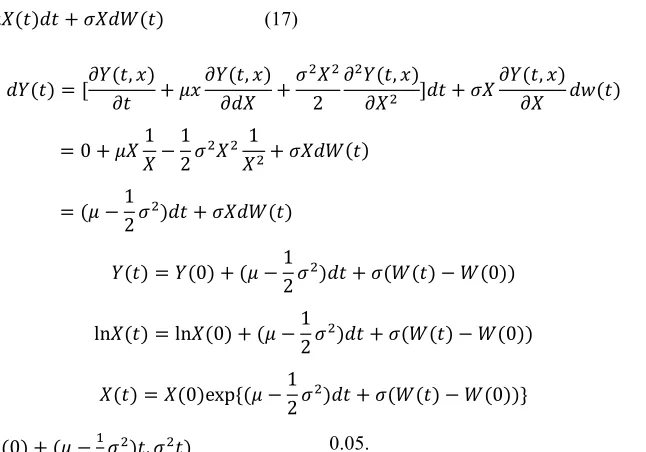
Geometric Brownian Motion (GBM). The SDE for GBM is given as:
C2( ) = B2( )C + D2C,( ) (17)
Using ito’s lemma to solve the SDE (16). Let, £ =ln2
C£ !∂£ ,
∂ @ B
∂£ ,
∂C2 @
DU2U 2
∂U£ ,
∂2U QC @ D2
∂£ ,
∂2 C¥
0 @ B21
2
-1 2DU2U
1
2U@ D2C,
B -1
2DU C @ D2C,
£ £ 0 @ B -1
2DU C @ D , - , 0
ln2 ln2 0 @ B -1
2DU C @ D , - , 0
2 2 0 exp B -1
2DU C @ D , - , 0 $
Hence, 2 ~¦1 ln2 0 @ B -|
UD U , DU
This means that the log transform of Debt Ratio is normally distributed. Using historical data on debt Ratio, we transformed the data to log and tested normality of the transformed data using QQ-plot and shapiro test since the test is more sensitive to small sample size.
4.3.3. Normality Test
The null hypothesis for the shapiro-Wilk test for normality is:
§/: The data is normally distributed.
The null Hypothesis is rejected if the p-value is less than
0.05.
Table 1. Shapiro-Wilk Normality Test.
Data Log (Debt Ratio)
W = 0.96489 P-value = 0.3027
Since P-value is greater than 0.05, the null hypothesis is not rejected hence normality of data is assumed.
The QQ-plot for the data is given in figure 1.
Figure 1. QQ-Plot.
We estimate the parameters from the transformed historical data. Given that,
C2
2 BΔ @ D©√Δ
This means that,
C2
2 ~1 BΔ , D√Δ
estimate of D√Δ .
From the data, the parameter B is 0.039 while the parameter D is 0.1134.
4.4. Results and Discussion
We set the parameter values that we will consider in our analysis.
Table 2. Parameter Values.
k ¬ - n ® ¯ ° r g
1 0.04 0.11 2 0.51 0.095 0 0.07 0.03
In the table above, we have set the basic parameter values that we are going to use in our analysis. We recall the meaning of these parameters: B = (E − F) is the difference between real interest rate and the economic growth rate, D is the debt ratio volatility, k is the marginal cost of intervention, n is aversion towards debt, T represents characteristics of the debt, scale parameter W and risk free rate, R.
To use the explicit formula for the optimal debt ceiling, we assume that the parameters, g, economic growth rate, and r, interest rate, are constant parameters. D represents volatility in the debt dynamics. This means that the debt ratio can increase or decrease due to deficits or surpluses that are beyond the government control.
Using parameters set in the table above we calculate the value of the optimal debt ceiling, b and the corresponding
value function as shown below. The optimal debt ceiling is given by:
{ = (−T‘2 (2 − 1) + T‘2 (”UP(”U− 1) − 1))UVM||
{ = 0.2782979
Hence, using the specific parameters for Kenya, the optimal debt ceiling is 27.82979%. This means that when the debt ratio is at 27.8% and crosses the optimal debt ceiling, the government should put fiscal adjustments measures in place to control the debt ratio from crossing b. If the initial debt ratio x is greater than the debt ceiling, b, the control process Z, jumps from /= 0 to /= − {. In the same manner, the debt ratio transits from 2/= to 2/= {. Therefore, if > {, the fiscal adjustments measures should be taken to increase the primary surplus by ( − {).
Therefore, at any period when the debt ratio of Kenya is below 27.82979%, no fiscal interventions are needed; if the debt ratio equals 27.82979%, then control should be put in place to prevent it from crossing b; if 27.82979%, then the government should immediately put control measures that aim at lowering the debt ratio to the optimal level.
Using the values given in the table above, the value function corresponding to the optimal government debt ceiling 27.82979% is
( ) = 2.875095 |.¶·¸U/¹− 0.51
8.759838 ¸ < 0.2782979 − 0.02981958 ≥ 0.2782979
The value function is gives the smallest expected total cost. By total cost we mean, the sum of the cost of having the debt and the intervention cost. The value function gives the minimum cost that can be obtained when the initial debt ratio is x and all acceptable controls are considered.
For instance in 2016, the debt ratio for Kenya was 0.5263393. The value function associated with the debt ratio, x is P + “ since > 0.2782979. This implies that the minimum expected total cost the government incurred is 0.497 i.e. (0.5263393-0.02981958).
On the other hand, we consider a case in which <
0.2782979. In 2008, the debt ratio for Kenya was 0.2628896 hence below the optimal debt ceiling. The value function associated with this ratio is given by 2.875095 |.¶·¸U/¹−
/.»|
¶.¼»½¶·¶ ¸ which evaluates to a minimum expected cost of
0.247691.
This implies that the government incurs a higher cost when the debt ratio ≥ optimal debt ceiling than when the debt ratio
< optimal debt ceiling.
5. Conclusion and Recommendation
5.1. Conclusion
The study aimed at establishing the optimal debt ceiling
for Kenya and the corresponding value function. To achieve this we used an explicit formula for optimal debt ceiling. We chose to use the formula because it is a function of macroeconomic variables such as the economic growth, interest rate, debt volatility, debt aversion, risk free rate that are unique for each country. This implies that using a particular country’s data it is possible to use the formula to determine the optimal debt ceiling for that country.
From the study, we established that the volatility of debt dynamics in Kenya is 0.01134. This means that the Kenyan debt ratio can increase or decrease by 0.01134 due to factors beyond the control of government.
We found out that the optimal debt ceiling for Kenya is 27.82979%. This means that at any point when the debt ratio is above 27.82979%, the government incurs an intervention cost in addition to the running cost of having a debt. This was illustrated in the study where we found out that the value function was higher in cases when the debt ratio, x, was greater than the optimal debt ceiling, b, and vice-versa. This additional cost can have negative effects in the economy such as tax distortion due to increased taxation and less growth of capital stock.
recently downgraded Kenya from B2 to B1 due to a rise in debt levels and deterioration in debt afford-ability (Moody’s, 2018). At the time of downgrade, Kenya’s debt ratio was at 54%. This downgrade is consistent with the findings of this study that indicate that the debt ratio in Kenya is above the optimal debt ceiling. Hence, the government should take fiscal adjustments measures aimed at maintaining the debt ratio at or below the optimal debt ceiling.
The novel aspects covered in this study are:
1. In calculating the value of the subjective parameterT, which represents the characteristics of a country’s Public debt, we obtained the ratio of cumulative domestic debt and foreign debt to total public debt. Cumulatively, the ratio of cumulative domestic debt and foreign debt to total public debt was 0.49: 0.51. We hence set the value of T to 0.51 to reflect the dominance of total public debt by foreign debt.
2. Further, we used the Central Bank risk-free Rate rather the Discount rate because the variable is usually determined by an autonomous Central Bank, whose action is not modelled in the model.
5.2. Recommendation for Further Study
This study has used one dimensional stochastic optimal control model for study of optimal debt ceiling. A more comprehensive multidimensional approach could be used to determine the optimal debt ceiling. For the multidimensional approach, the debt dynamics would depend on macroeconomic factors such as exchange rate and inflation that would be modelled exogenously.
References
[1] Soner, Stochastic Optimal Control in Finance., Oxford, 2004. [2] K. Ross, Stochastic Control in Continuous time, Stanford
University.
[3] Cadenillas and Aguilar, "Explicit formula for the optimal government debt ceiling," Annals of Operation Research, vol. 247, no. 2, pp. 415-449., 2016.
[4] N. Treasury, "Annual Public Debt Management Report, Kenya," Nairobi, 2016.
[5] Wyplosz, "Fiscal policy: institutions versus rules.," National Institute Economic Review 191 6478, 2005.
[6] Merton, "Optimum Consumption and Portfolio Rules," JOURNAL OF ECONOMIC THEORY, vol. 3, pp. 373-413, 1971.
[7] Z. Wei-han, Analysis of Optimal Debt Ratio in A Markov Regime-Switching Model, 2014.
[8] S. Pontryagin, "optimal processes of regulation, UspekhiMat.," English transl. in American Mathematical Society Transl, vol. 1, no. 85, p. 320, 1959.
[9] R. Bellman, Dynamic Programming, Princeton Univ., Press, Princeton, New Jersey., 2010.
[10] Yong et al, Stochastic Controls: Hamiltonian Systems and HJB Equations, Springer, New York., 1999.
[11] Ferrari, "On the Optimal Management of Public Debt: a Singular Stochastic Control Problem, to appear in SIAM," 2016. [Online]. Available: https://arxiv.org/abs/1607. 04153. [Accessed 02 04 2018].
[12] Ostry et al, "IMF Staff Discussion note, When Should Public Debt Be Reduced?" IMF, 2015.
[13] Stein, Stochastic optimal control, international finance and debt crises, Oxford University Press., 2012.
[14] Barro, "Notes on optimal debt management.," Journal of Applied Economics, vol. 2, no. 2, p. 281289., 1999.
[15] Barro, "(1974), Are government bonds net wealth?" The Journal of Political, 1974.