Refbacks

(1)

Is Management

a Science

or an Art?

From Theory

to Practice

of Management

5

DOI: 10.17951/ijsr.2017.6.5

Is Management a Science or an Art?

From Theory to Practice of Management

Wiesław M. Grudzewski

Associate member of the Polish Academy of Sciences (PAN)

Zoia Wilimowska

University of Applied Sciences in Nysa, Poland

[email protected]

Abstract

Purpose – The purpose of this article is to discuss and show that management is a science, not just an art. Decision-making in the enterprise requires talent and special skills supported by the right qualiications. According to Tatarkiewicz, management can be considered as an art, which can be interpreted as follows: “(...) man’s conscious creation is a work of art always when it recreates reality, shapes forms, or expresses experience, yet it is able either to delight, or touch, or shock” (Tatarkiewicz, 1972). On the other hand, the company management is understood as a continuous process of making decisions based on reliable knowledge, observations and experiences – it is, therefore, a science, and modern managers are not just passive consumers of research knowledge, but also its creators. Contemporary theories focus attention on constructing appropriate models, which support the decisions of managers allowing them to somehow “spy” and observe the effects of their decisions. The aim of the paper is to show that in the modern economy, design models to support the management of the enterprise is the science that uses the achievements of other sciences, creative adaptation of these achievements in modeling phenomena occurring in the world economy. The aim of this article is to show that management sciences are increasingly exploiting modern knowledge to build models for developing practical concepts of management systems.

Design/Methodology/Approach – The authors present the review of mathematical models, computer models (used in situations where the analytical models cannot ind the best solution), and in particular artiicial intelligence algorithms and selected models of dynamic system for managing the organization and some examples of applications.

Findings – The results obtained show that in the management sciences, many models are used to support managerial decisions. Of course, the achievements of other sciences are very often used, management is of an application, but also of scientiic nature, because, in order to skillfully use knowledge from other ields, decision-making models should be developed to solve problems in management and allow to use the achievements of these other areas.

Research limitations/implications – The limitations of this paper result from the fact that only selected models are presented in the article. The authors hope that these selected models will be the argument that management science is becoming more and more science and not an art only.

Originality/Value – This paper presents the review of modern methods used in management sciences to show that modern management is more a science than an art.

Keywords – management, models, artiicial intelligence, neural networks, agent, risk

International Journal of Synergy and Research

Vol. 6, 2017 pp. 5–21

Pobrane z czasopisma International Journal of Synergy and Research http://ijsr.journals.umcs.pl Data: 08/09/2020 10:05:27

(2)

6 IJSR

6 1. Introduction

In the market economy, management of any enterprise is of particular importance because its appropriate implementation ensures the proper growth and development of an enterprise. The management process consists mainly of continuous decision-making. Whether managerial decisions will ensure eficiency or improve the company’s image, it is dificult to determine at the time when the decisions are made. The effects of decisions are only observable in the future, sometimes very distant. Making decisions determining the company’s future and goals accomplishment requires a thorough knowledge in many areas (decision-making, inancial management, risk assessment, forecasting, etc.) and experience as well as creative capabilities of decision-makers.

Then, is management art or science?

According to the Polish Language Dictionary [II], art “is an area of artistic activity distinguished for its aesthetic values; also a product/creation or products of such activities, but also the ability requiring talent, skill or special qualiications”. The creator is any person [III] “who creates something, especially in the ield of art, or a person who is the cause of something”.

Decision-making in the enterprise requires talent and special skills supported by the accurate qualiications. In this context, management is an art that can be interpreted as (Tatarkiewicz, 1972) “the conscious work of a human being [which] is considered a work of art always and only when it recreates reality, shapes forms, or expresses experience, and, at the same time, is fascinating, emotional, or even shocking”.

The Polish dictionary by PWN deines science as [IV] “All human knowledge arranged in the system of issues; also: the discipline of research relating to a certain ield of reality” or “A set of views that constitute a systematized and consistent whole and are part of a particular discipline of research”.

In this context, the company’s management understood as a continuous decision-making process based on sound knowledge, observation and experience is science, and modern managers are not just passive consumers of research knowledge but also its creators.

These theories include, among others, the quantiied theory of a production function and the ways it is created in national economies and particular branches of production. There is also the theory of strategic and operational management, organisational balance, assessment stimulation and measurement of a function of demand and supply, trust management, management of enterprises under conditions of uncertainty, knowledge management, measurement of technological and technical gaps in national economies and economic sectors, and other well-known theories such as the application of Danzig’s programming and linear algorithm to solve transport problems, network planning for programming and implementing projects in construction services and restoration of facilities, sustainability in business (Grudzewski et al., 2013), crisis management, creation of a company in the future, dynamic programming applied to create decision-making systems in processes and management systems, probability calculus/theory in mass/multiple service management such as telephone exchanges or rental of apparatus, devices and measuring tools in scientiic research, conducting experiments and designing projects applied in business practice. The number of these theories is growing, and their practical use becomes the basis for the improvement

(3)

Is Management

a Science

or an Art?

From Theory

to Practice

of Management

7

of strategic and operational management systems in economics. On the basis of these theories, organizational and process structures as well as IT networks are developed to process information in systems that use a large number of algorithms to enable practical problem-solving. Various models are available for this purpose such as mathematical, static, and dynamic models: deterministic, stochastic, fuzzy, network, cybernetic, IT, iconographic, etc.

2. Models in management systems

Uncertainty in the decision-making process depends on the dynamics of changes in the business environment as well as the degree of conidence in the opinions, ideas, solutions that the decision-maker makes, etc. It is dificult, costly, and often even impossible to undertake experiments and test the potential effects of decisions on a living organism, just like an enterprise. Hence, contemporary theories focus on constructing appropriate models that support managerial decisions, allowing them to “view/track” the effects of their decisions. The main purpose of modelling is to understand how a company operates as well as to analyse its performance and propose possible improvements.

The study of processes and systems can take place on real objects/assets or on models. The investigated actual/current system is a fragment of the environment, while the model is merely a simpliied representation of the examined part of reality containing a certain number of its properties relevant for the research conducted.

Modelling supports and motivates mental imagery and knowledge about possible future consequences, and, thus, facilitates inding a goal. It allows one to verify the reliability and feasibility of the system’s objectives with respect to the values and expectations of the environment, as well as evaluate the technical usability in particular aspects of: structure, functionality, time, society and economics.

Taking into account the complexity of enterprise management, the rationality of managerial decisions requires a prior analysis of the potential impact of decisions, thus, requires modelling of decision-making processes.

One of the most important tasks implemented by modelling phenomena and processes is to ind the best solutions in complex reality.

3. Mathematical models

Finding the best solutions to speciic problems is as old as the history of civilization. This inds its justiication in the pursuit of man to perfection. In the history of Carthage, in the Aeneid by Virgil [70–19 BC], there is the phrase “ind a curve closed on a plane of a given length, which contains the maximum surface”.

Over more than 300 years, people have sought some formalized methods to ind the best solutions. At the end of the 17th_{century, Johann Bernoulli announced a competition}

to solve the following problem: “Given two points A and B in a vertical plane, what is the curve traced out by a point acted on only by gravity, which starts at A and reaches B in the shortest time.” There were several solutions provided by famous mathematicians. Thus, the period of development of the mathematical analysis and the search for optimal analytical solutions that require strictly mathematical models began.

(4)

8 IJSR

6

A mathematical model is a set of rules and relationships, based on which the course of a modelled process can be foreseen (by way of calculation). The mathematical model of the studied material/tangible system will be called the system of equations whose solutions are similar to the course of the modelled actual object size/dimension.

The advantage of mathematical models is their abstract character; an identical mathematical model may have systems and processes of different physical nature, and this particular feature of mathematical models is of particular interest. Searching for optimal solutions using mathematical models requires precise formulation of the model. An enterprise is a complex system. In order to construct the best model for the type of decision-making process in question, in subject-related literature and practice, it is proposed to decompose the system.

3.1. The examples of company risk evaluation

The organizational environment is becoming more dynamic and unpredictable, and, therefore, organizations are required to monitor their environment continually and adapt to it.

Many social groups are interested in the effects of company’s operation. And each group is interested in various types of risk of organization activity. There is no proit without risk. Generally speaking, risk is a concept that denotes a potential negative impact that may arise from a future event, especially a total or partial loss of invested resources.

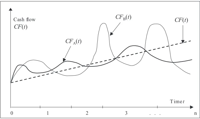
Risk can be understood as a possibility that actual cash lows generated by the company will be less than forecasted cash lows – actual rate of return will be less than expected required return because of variability and unpredictability of the cash

Figure 1.

Variability of cash lows for A and B irms

4 The advantage of mathematical models is their abstract character; an identical mathematical

model may have systems and processes of different physical nature, and this particular feature

of mathematical models is of particular interest. Searching for optimal solutions using

mathematical models requires precise formulation of the model.

An enterprise is a complex system. In order to construct the best model for the type of

decision-making process in question, in subject-related literature and practice, it is proposed

to decompose the system.

3.1. The examples of company risk evaluation

The organizational environment is becoming more dynamic and unpredictable, and, therefore,

organizations are required to monitor their environment continually and adapt to it.

Many social groups are interested in the effects of company’s operation. And each

group is interested in various types of risk of organization activity. There is no profit without

risk. Generally speaking, risk is a concept that denotes a potential negative impact that may

arise from a future event, especially a total or partial loss of invested resources.

Risk can be understood as a possibility that actual cash flows generated by the

company will be less than forecasted cash flows

–

actual rate of return will be less than

expected required return because of variability and unpredictability of the cash flow levels

CF

i

in future time periods (Figure 1) (Wilimowska, Wilimowski, 2002). If required level of

cash flow is a linear function of time CF(t) (then the risk connected with variability of cash

flow is zero, and growing level of cash flow increases investment profitability), then for

investment A variability of CF

A

(t) is greater, so the risk is greater. For investment B cash flow

CF

B

(t) is the least stable

–

it causes the greatest risk.

Time Cash flow

0 1 2 3 . . . n

t

CF(t)

CFB(t)

CFA(t)

CF(t)

Figure 1. Variability of cash flows for A and B firms Source: Wilimowska and Wilimowski (2002).

Source: Wilimowska and Wilimowski (2002).

(5)

Is Management

a Science

or an Art?

From Theory

to Practice

of Management

9

low levels CFi in future time periods (Figure 1) (Wilimowska, Wilimowski, 2002). If

required level of cash low is a linear function of time CF(t) (then the risk connected with variability of cash low is zero, and growing level of cash low increases investment proitability), then for investment A variability of CFA(t) is greater, so the risk is greater.

For investment B cash low CFB(t) is the least stable – it causes the greatest risk.

The factors that determine company’s value which exists in dynamically changing environment and inluencing the forecasted cash low level are not deterministic. They follow the unpredicted environment changes and internal changes of the company. So the factors should have non-deterministic character in valuation process.

3.2.Discrete method of risk evaluation

As was mentioned before, there is no proit without risk. Generally speaking, risk is a concept that denotes a potential negative impact that may arise from a future event, especially a total or partial loss of invested resources.

The risk of the company evaluation problem can be deined as follows (Wilimowska, 2004): to classify a company to one of M risk classes – 1, 2, ..., M using some factors describing it. Depending on the type and quantity of input information, two tasks are considered:

• number of risk classes is known, • number of risk classes is unknown.

The tasks can be resolved using cluster analysis and pattern recognition theory, respectively. In the risk classiication task, points of the feature space are irms described in vectors of features terms. Process of discrete inancial risk measuring shows Figure 2.

5 The

factors that determine company’

s value which exists in dynamically changing

environment and influencing the forecasted cash flow level are not deterministic. They follow

the unpredicted environment changes and internal changes of the company. So the factors

should have non-deterministic character in valuation process.

3.2.Discrete method of risk evaluation

As was mentioned before, there is no profit without risk. Generally speaking, risk is a concept

that denotes a potential negative impact that may arise from a future event, especially a total

or partial loss of invested resources.

The risk of the company evaluation problem can be defined as follows (Wilimowska,

2004): to classify a company to one of

M

risk classes

–

1, 2, ...,

M

using some factors

describing it. Depending on the type and quantity of input information, two tasks are

considered:



number of risk classes is known,



number of risk classes is unknown.

The tasks can be resolved using cluster analysis and pattern recognition theory,

respectively. In the risk classification task, points of the feature space are firms described in

vectors of features terms. Process of discrete financial risk measuring shows Figure 2.

Figure 2. Scheme of risk classification

The main problem of right classification is to find the proper function of

H(x)

transforming the feature vector in a particular class

i

0

. There are many methods of pattern

recognition and classification theory. The methods depend on the type of information that is

known before.

Let us assume that objects in each

M

classes are random variables and

p(x/i) i

= 1, ...,

M

are their

a priori

conditional probability functions. Let us assume that

p

i

, i

= 1, ...,

M

are

a

priori

probabilities of class

i

respectively. If probability distributions

p(x/i)

and

p

i

, i

= 1, ...,

M

exist and are known, than full probabilistic information about objects and classes is known.

Using a statistical theory of decision making there is possible loss functions defining



(

i/j

)

i

,

j

= 1, ...,

M

, which represent losses of incorrect classifying of object

i

to wrong class

j

.

Let us describe

p

(

j

/

x

) as

a posteriori

probability that

x

belongs to class

j

. Then

L i

_x

i j

j x

j M

( )



( / ) ( / )







p

1

The main problem of right classiication is to ind the proper function of H(x) transforming the feature vector in a particular classi₀. There are many methods of pattern recognition and classiication theory. The methods depend on the type of information that is known before.

Let us assume that objects in each M classes are random variables and p(x/i) i = 1, ..., M are their a priori conditional probability functions. Let us assume that p_i, i = 1, ..., M are a priori probabilities of class i respectively. If probability distributions p(x/i) and p_i, i = 1, ..., M exist and are known, than full probabilistic information about objects and classes is known.

Using a statistical theory of decision making there is possible loss functions deining λ(i/j) i, j = 1, ..., M, which represent losses of incorrect classifying of object i to wrong class j.

Figure 2.

Scheme of risk classiication

(6)

10 IJSR

6

Let us describe p(j/x) as a posteriori probability that x belongs to class j. Then

5

The factors that determine company’s value which exists in dynamically changing environment and influencing the forecasted cash flow level are not deterministic. They follow the unpredicted environment changes and internal changes of the company. So the factors should have non-deterministic character in valuation process.

3.2.Discrete method of risk evaluation

As was mentioned before, there is no profit without risk. Generally speaking, risk is a concept that denotes a potential negative impact that may arise from a future event, especially a total or partial loss of invested resources.

The risk of the company evaluation problem can be defined as follows (Wilimowska, 2004): to classify a company to one of M risk classes – 1, 2, ..., M using some factors describing it. Depending on the type and quantity of input information, two tasks are considered:

 number of risk classes is known,

 number of risk classes is unknown.

The tasks can be resolved using cluster analysis and pattern recognition theory, respectively. In the risk classification task, points of the feature space are firms described in vectors of features terms. Process of discrete financial risk measuring shows Figure 2.

Figure 2. Scheme of risk classification

The main problem of right classification is to find the proper function of

H(x)transforming the feature vector in a particular classi0. There are many methods of pattern recognition and classification theory. The methods depend on the type of information that is known before.

Let us assume that objects in each M classes are random variables and p(x/i) i = 1, ...,

M are their a priori conditional probability functions. Let us assume that pi, i = 1, ..., M are a

priori probabilities of class i respectively. If probability distributions p(x/i) and pi, i = 1, ..., M exist and are known, than full probabilistic information about objects and classes is known. Using a statistical theory of decision making there is possible loss functions defining

(i/j) i, j = 1, ..., M, which represent losses of incorrect classifying of object i to wrong class j. Let us describe p(j/x) as a posteriori probability that x belongs to class j. Then

L ix i j j x

j M

( ) ( / ) ( / ) 



 p

1

is an average conditional loss.

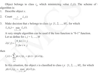
Object belongs to class i₀, which minimizing value L_x(i). The scheme of the algorithm is:

1. Describe object x. 2. Count

6

Object belongs to class i0, which minimizing value Lx(i). The scheme of the algorithm

is:

1. Describe object x. 2. Count 



i 1 2, ,...,M xL i( )

3. Make decision that x belongs to class i0{1, 2, ..., M}, for which

L ix L i

i M x

( ) min ( )

,..., 0

1



 .

A very simple algorithm can be used if the loss function is “0-1” function.

Let us define for i, j = 1, ..., M

  

 

 ₁0 _.

) / ( j i for j i for j i  then

l ix x j j x x i

j j i M i ( ) ( / )  ( ) ( / )  



p p p p p .

1

In this situation, the object x is classified to class io {1, 2, ..., M}, for which

p(x/io)pio _i_max₁_,...,_Mp(x/i) pi.

To classes of risk defining, the agglomeration method of cluster analysis can be used.

The example

The objective of the research is to classify selected companies to some classes of risk at the base of 4 characteristics (four financial ratios) (Wilimowska et al., 2016).

For this purpose, the agglomeration method will be used for number of class definition. The result of this method is the tree of connections, the so-called dendrogram. Using the method of agglomeration, the researcher subjectively determines the number of classes (clusters) setting the line of intersection of the tree.

In the example, dendrogram was constructed using the method of Ward and the Euclidean distance, which were used to determine the cluster for selected financial ratios. The results of the cluster analysis are shown in Figure 3.

3. Make decision that x belongs to class i0∈{1, 2, ..., M}, for which

6

is:

1. Describe object x.

2. Count  

i 1 2, ,...,M xL i( )

L i_x L i

i M x

( ) min ( )

,..., 0

1



 .

  

 

 ₁0 _.

j j i M i ( ) ( / )  ( ) ( / )  



p p p p p .

1

p(x/io)p_i

i M

o  _max₁_,..., p(x/i) pi.

The example

A very simple algorithm can be used if the loss function is “0-1” function. Let us deine for i, j = 1, ..., M

6

is:

2. Count  

i 1 2, ,...,M xL i( )

L ix L i

i M x

( ) min ( )

,..., 0

1



 .

  

 

 ₁0 _.

j j i M i ( ) ( / )  ( ) ( / )  



p p p p p .

1

p(x/io)p_i

i M

o  _max₁_,..., p(x/i) pi.

The example

then

6

is:

2. Count  

i 1 2, ,...,M xL i( )

L ix L i

i M x

( ) min ( )

,..., 0

1



 .

  

 

 ₁0 _.

j j i M i ( ) ( / )  ( ) ( / )  



p p p p p .

1

p(x/io)p_i

i M

o _max₁_,..., p(x/i) pi.

The example

In this situation, the object x is classiied to class i_o∈ {1, 2, ..., M}, for which

6

is:

2. Count  

i 1 2, ,...,M xL i( )

L ix L i

i M x

( ) min ( )

,..., 0

1



 .

  

 

 ₁0 _.

j j i M i ( ) ( / )  ( ) ( / )  



p p p p p .

1

p(x/io)pio _i_max₁_,...,_Mp(x/i) pi.

The example

To classes of risk deining, the agglomeration method of cluster analysis can be used.

The example

The objective of the research is to classify selected companies to some classes of risk at the base of 4 characteristics (four inancial ratios) (Wilimowska et al., 2016).

For this purpose, the agglomeration method will be used for number of class deinition. The result of this method is the tree of connections, the so-called dendrogram. Using the method of agglomeration, the researcher subjectively determines the number of classes (clusters) setting the line of intersection of the tree.

In the example, dendrogram was constructed using the method of Ward and the Euclidean distance, which were used to determine the cluster for selected inancial ratios. The results of the cluster analysis are shown in Figure 3.

So, ive classes were deined. The irst class consists of the companies that have a good inancial condition – small level of risk. The second class is composed of the companies that are characterized by a suficient inancial condition. In contrast, the companies which have a frail inancial condition are in the third class. On the other hand, the fourth class consists of companies with a very bad inancial condition – high level of risk. The last class, ifth, is composed of companies with a critical inancial condition – the highest level of risk.

(7)

Is Management

a Science

or an Art?

From Theory

to Practice

of Management

11

A priori probabilities for 5 classes are calculated based on the percentage of announced bankruptcy of economic entities in relation to the total deleted companies from REGON register. Therefore, the a priori probability of class 1, 2, 3 is 0.31 and for class 4 and class 5 it is 0.035.

Results of the Kolmogorov–Smirnov test and histogram igures of numerous layouts of tested ratios in the class were calculated by computer program STATISTICA. The tests for features for bad and good inancial condition of companies, showed that probability density functions are normal.

Using the formula for normal probability density function and calculated parameters, for each feature here, conditional probability density function was calculated , where i = 1, 2, 3, 4 (number of features); j = 1, 2, 3, 4, 5 (number of classes).

Under the assumption that features are independent, total conditional probability density function is:

7

Figure 3. Cluster analysis using the methods of agglomeration Source: Wilimowska et al. (2016).

So, five classes were defined. The first class consists of the companies that have a good financial condition – small level of risk. The second class is composed of the companies that are characterized by a sufficient financial condition. In contrast, the companies which have a frail financial condition are in the third class. On the other hand, the fourth class consists of companies with a very bad financial condition – high level of risk. The last class, fifth, is composed of companies with a critical financial condition – the highest level of risk.

A priori probabilities for 5 classes are calculated based on the percentage of

announced bankruptcy of economic entities in relation to the total deleted companies from REGON register. Therefore, the a priori probability of class 1, 2, 3 is 0.31 and for class 4 and class 5 it is 0.035.

Results of the Kolmogorov–Smirnov test and histogram figures of numerous layouts of tested ratios in the class were calculated by computer program STATISTICA. The tests for features for bad and good financial condition of companies, showed that probability density functions are normal.

Using the formula for normal probability density function and calculated parameters, for each feature here, conditional probability density function was calculated �(��|�), where i

= 1,2,3,4 (number of features); j = 1, 2, 3, 4, 5 (number of classes).

    

x

j

f

x

j

f

x

j

   

f

x

j

f

x

j



f

|



1

|

*

2

|

*

3

|

*

4

|

, j = 1, 2, 3, 4, 5.

That means:

 

_





 _

 

  _ _  4

1 2

2

2 exp 2

2 1 |

i ij

ij i

ij

x x j

x f



, j = 1, 2, 3, 4, 5.

That means:

7

Figure 3. Cluster analysis using the methods of agglomeration

Source: Wilimowska et al. (2016).

So, five classes were defined. The first class consists of the companies that have a good financial condition – small level of risk. The second class is composed of the companies that are characterized by a sufficient financial condition. In contrast, the companies which have a frail financial condition are in the third class. On the other hand, the fourth class consists of companies with a very bad financial condition – high level of risk. The last class, fifth, is composed of companies with a critical financial condition – the highest level of risk.

A priori probabilities for 5 classes are calculated based on the percentage of announced bankruptcy of economic entities in relation to the total deleted companies from REGON register. Therefore, the a priori probability of class 1, 2, 3 is 0.31 and for class 4 and class 5 it is 0.035.

Results of the Kolmogorov–Smirnov test and histogram figures of numerous layouts of tested ratios in the class were calculated by computer program STATISTICA. The tests for features for bad and good financial condition of companies, showed that probability density functions are normal.

Using the formula for normal probability density function and calculated parameters, for each feature here, conditional probability density function was calculated �(��|�), where i

= 1,2,3,4 (number of features); j = 1, 2, 3, 4, 5 (number of classes).

    

x j f x j f x j

   

f x j f x j



f |  1| * 2| * 3| * 4| , j = 1, 2, 3, 4, 5.

That means:

 

_





 

   

 

_ _

 4

1 2

2

2exp ₂

2 1 |

i ij

ij i

ij

x x j

x f



 , j = 1, 2, 3, 4, 5.

Figure 3.

Cluster analysis using the methods of agglomeration Source: Wilimowska et al. (2016).

(8)

12 IJSR

6

Where: 8 Where:

��– standard deviation of i-feature of j-class;

��– expected value of i-feature of j-class;

�� –i-feature of classified object.

Remembering that Bayes’ algorithm needs a value ofpjf(x/j), calculation for each class and choosing the maximum value of that a posteriori probability of class, the results of classification shows Table 1.

Table 1. The examples of classification by Bayes’ model

Company Real Class Result of class 1

Result of class 2

Result of class 3

Result of class 4

Result of class 5 Class

Copal 1–3 0.996 0.004 0.000 0.000 0.000 1

Androimpex 1–3 0.001 0.542 0.457 0.000 0.000 2

Azomet Sp. z o.o. 4–5 0.000 0.000 0.000 1.000 0.000 4

B.P. Print Sp. z o.o. 4–5 0.000 0.000 0.000 1.000 0.000 4

… 4–5 0.000 0.000 0.002 0.998 0.000 4

Bełchatowskie Zakłady Przemysłu Bawełnianego Sp. z

o.o. 4–5 0.000 0.000 0.000 0.000 1.000 5

3.3. Fractal model in risk modelling

The fractal dimension was defined by Mandelbrot during the study of Great Britain’s

coastline. Thanks to this research, he noted that the coastline is not an object Euclidean, so its dimension cannot be described by an integer of 2 (Mandelbrot, 1967). The entire coastline was covered with N circles having the same radius – r. These measurements were repeated reducing and increasing the radius. It turned out that every time it was obtained the following equivalence relation:

�(2 ∗ �)� _{= 1}

Where: N – number of circles, r – radius of circles, D – fractal dimension.

So, the fractal dimension is:

� = log � �� (_2�1) – standard deviation of i-feature of j-class;

8 Where:

Result of class 2

Result of class 3

Result of class 4

Copal 1–3 0.996 0.004 0.000 0.000 0.000 1

Androimpex 1–3 0.001 0.542 0.457 0.000 0.000 2

Azomet Sp. z o.o. 4–5 0.000 0.000 0.000 1.000 0.000 4

B.P. Print Sp. z o.o. 4–5 0.000 0.000 0.000 1.000 0.000 4

… 4–5 0.000 0.000 0.002 0.998 0.000 4

o.o. 4–5 0.000 0.000 0.000 0.000 1.000 5

�(2 ∗ �)� _{= 1}

� = log � �� (_2�1) – expected value of i-feature of j-class;

8 Where:

Result of class 2

Result of class 3

Result of class 4

Copal 1–3 0.996 0.004 0.000 0.000 0.000 1

Androimpex 1–3 0.001 0.542 0.457 0.000 0.000 2

Azomet Sp. z o.o. 4–5 0.000 0.000 0.000 1.000 0.000 4

B.P. Print Sp. z o.o. 4–5 0.000 0.000 0.000 1.000 0.000 4

… 4–5 0.000 0.000 0.002 0.998 0.000 4

o.o. 4–5 0.000 0.000 0.000 0.000 1.000 5

�(2 ∗ �)� _{= 1}

� = log � �� (_2�1) – i-feature of classiied object.

Remembering that Bayes’ algorithm needs a value of

p

_j

f

(

x

/

j

)

, calculation for each class and choosing the maximum value of that a posteriori probability of class, the results of classiication shows Table 1.

Company Real Class Result of class 1 Result of class 2 Result of class 3 Result of class 4 Result of class 5 Class

Copal 1–3 0.996 0.004 0.000 0.000 0.000 1

Androimpex 1–3 0.001 0.542 0.457 0.000 0.000 2

Azomet Sp. z o.o. 4–5 0.000 0.000 0.000 1.000 0.000 4

B.P. Print Sp. z o.o. 4–5 0.000 0.000 0.000 1.000 0.000 4

… 4–5 0.000 0.000 0.002 0.998 0.000 4

Bełchatowskie Zakłady Przemysłu

Bawełnianego Sp. z o.o. 4–5 0.000 0.000 0.000 0.000 1.000 5

3.3. Fractal model in risk modelling

The fractal dimension was deined by Mandelbrot during the study of Great Britain’s coastline. Thanks to this research, he noted that the coastline is not an object Euclidean, so its dimension cannot be described by an integer of 2 (Mandelbrot, 1967). The entire coastline was covered with N circles having the same radius – r. These measurements were repeated reducing and increasing the radius. It turned out that every time it was obtained the following equivalence relation:

8 Where:

Result of class 2

Result of class 3

Result of class 4

Copal 1–3 0.996 0.004 0.000 0.000 0.000 1

Androimpex 1–3 0.001 0.542 0.457 0.000 0.000 2

Azomet Sp. z o.o. 4–5 0.000 0.000 0.000 1.000 0.000 4

B.P. Print Sp. z o.o. 4–5 0.000 0.000 0.000 1.000 0.000 4

… 4–5 0.000 0.000 0.002 0.998 0.000 4

o.o. 4–5 0.000 0.000 0.000 0.000 1.000 5

�(2 ∗ �)� _{= 1}

� = log � �� (_2�1)

Where: N – number of circles, r – radius of circles, D – fractal dimension. So, the fractal dimension is:

8 Where:

Result of class 2

Result of class 3

Result of class 4

Copal 1–3 0.996 0.004 0.000 0.000 0.000 1

Androimpex 1–3 0.001 0.542 0.457 0.000 0.000 2

Azomet Sp. z o.o. 4–5 0.000 0.000 0.000 1.000 0.000 4

B.P. Print Sp. z o.o. 4–5 0.000 0.000 0.000 1.000 0.000 4

… 4–5 0.000 0.000 0.002 0.998 0.000 4

o.o. 4–5 0.000 0.000 0.000 0.000 1.000 5

�(2 ∗ �)�_{= 1}

� = log � �� (_2�1)

The more the object will be frayed and ragged, the more the fractal dimension approach will be close to the value of 2.

Hurst exponent, as a statistical measure used for deterministic fractal, is dependent only on the value of the correlation coeficient C between the pair tested parameters, which can be stored in the form (Kiłyk, Wilimowska, 2010; Czarnecka, Wilimowska, 2018):

9

Hurst exponent, as a statistical measure used for deterministic fractal, is dependent only on the value of the correlation coefficient C between the pair tested parameters, which can be stored in the form (Kiłyk, Wilimowska, 2010; Czarnecka, Wilimowska, 2018):

� = 2(2�−1)_{− 1}

Where: C – correlation coefficient, H – Hurst exponent.

So,

� =1_{2 (1 +}��_��2)

The possible value of Hurst exponent can be between 0 and 1.

When the value H is below 0.5, one can say that the analysed signal is anti-persistent, which means that there is a big probability that in the next step, it will be opposite to the current step. It is worth mentioning here that if the size takes a value closer to zero the more

“jagged” signal (more unpredictable, more risky). For a value H equal to 0.5, the signal is random and one can say that it is more like a Brownian motion.

The last interval for H is the value higher than 0.5. In this interval signal is persistent, which means there is a bigger probability that in the next step, the signal will behave like in the current step (trend will not be reversed). This means that the greater the value of H

assumed, the smoother the signal being analyzed (less unpredictable, less risky).

DMA method, as one of the few, is used for random fractals, which is difficult to define basic parameters. The main objective of the DMA method is that the signal fluctuations scaled accordingly with increasing scaling exponent (strongly dependent fractal dimension).

4. IT models

The concept of information system is found in subject-related literature quite often, however, it proves to be a very difficult task to define the concept precisely. In many scientific publications it is interpreted in an ambiguous way. Definitions of the information system given by different authors often vary from each other, but the idea and the essence of the information system remain rather unchanged. The variety of these definitions results from the fact that their authors postulate them according to purposes which the system is supposed to satisfy, and, above all, to the scientific disciplines they investigate. Studies dealing with the research on information systems are an interdisciplinary field because it includes, among others, IT issues, management sciences, sociology, and quantitative methods.

In Polish, the term “IT system” is quite misleading; another commonly used

expression is “EDP”, i.e. Electronic Data Processing. EDP concerns information processing rather than IT. IT is closely related to the technology itself and not to what it serves. It is the role of supporting business processes; IT itself is not a business process as some people think.

Where: C – correlation coeficient, H – Hurst exponent. Table 1.

The examples of classiication by Bayes’ model

(9)

Is Management

a Science

or an Art?

From Theory

to Practice

of Management

13

So,

9

Hurst exponent, as a statistical measure used for deterministic fractal, is dependent only on the value of the correlation coefficient C between the pair tested parameters, which can be stored in the form (Kiłyk, Wilimowska, 2010; Czarnecka, Wilimowska, 2018):

� = 2(2�−1)_{− 1}

Where: C – correlation coefficient, H – Hurst exponent.

So,

� =1_{2 (1 +}��_��2)

When the value H is below 0.5, one can say that the analysed signal is anti-persistent, which means that there is a big probability that in the next step, it will be opposite to the current step. It is worth mentioning here that if the size takes a value closer to zero the more

“jagged” signal (more unpredictable, more risky). For a value H equal to 0.5, the signal is random and one can say that it is more like a Brownian motion.

The last interval for H is the value higher than 0.5. In this interval signal is persistent, which means there is a bigger probability that in the next step, the signal will behave like in the current step (trend will not be reversed). This means that the greater the value of H

assumed, the smoother the signal being analyzed (less unpredictable, less risky).

DMA method, as one of the few, is used for random fractals, which is difficult to define basic parameters. The main objective of the DMA method is that the signal fluctuations scaled accordingly with increasing scaling exponent (strongly dependent fractal dimension).

4. IT models

The concept of information system is found in subject-related literature quite often, however, it proves to be a very difficult task to define the concept precisely. In many scientific publications it is interpreted in an ambiguous way. Definitions of the information system given by different authors often vary from each other, but the idea and the essence of the information system remain rather unchanged. The variety of these definitions results from the fact that their authors postulate them according to purposes which the system is supposed to satisfy, and, above all, to the scientific disciplines they investigate. Studies dealing with the research on information systems are an interdisciplinary field because it includes, among others, IT issues, management sciences, sociology, and quantitative methods.

In Polish, the term “IT system” is quite misleading; another commonly used

expression is “EDP”, i.e. Electronic Data Processing. EDP concerns information processing rather than IT. IT is closely related to the technology itself and not to what it serves. It is the role of supporting business processes; IT itself is not a business process as some people think.

When the value H is below 0.5, one can say that the analysed signal is anti-persistent, which means that there is a big probability that in the next step, it will be opposite to the current step. It is worth mentioning here that if the size takes a value closer to zero the more “jagged” signal (more unpredictable, more risky). For a value H equal to 0.5, the signal is random and one can say that it is more like a Brownian motion.

The last interval for H is the value higher than 0.5. In this interval signal is persistent, which means there is a bigger probability that in the next step, the signal will behave like in the current step (trend will not be reversed). This means that the greater the value of H assumed, the smoother the signal being analyzed (less unpredictable, less risky).

DMA method, as one of the few, is used for random fractals, which is dificult to deine basic parameters. The main objective of the DMA method is that the signal luctuations scaled accordingly with increasing scaling exponent (strongly dependent fractal dimension).

4. IT models

The concept of information system is found in subject-related literature quite often, however, it proves to be a very dificult task to deine the concept precisely. In many scientiic publications it is interpreted in an ambiguous way. Deinitions of the information system given by different authors often vary from each other, but the idea and the essence of the information system remain rather unchanged. The variety of these deinitions results from the fact that their authors postulate them according to purposes which the system is supposed to satisfy, and, above all, to the scientiic disciplines they investigate. Studies dealing with the research on information systems are an interdisciplinary ield because it includes, among others, IT issues, management sciences, sociology, and quantitative methods.

In Polish, the term “IT system” is quite misleading; another commonly used expres-sion is “EDP”, i.e. Electronic Data Processing. EDP concerns information processing rather than IT. IT is closely related to the technology itself and not to what it serves. It is the role of supporting business processes; IT itself is not a business process as some people think.

4.1.Genetic Algorithms (GA)

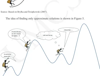
A Genetic Algorithm is a kind of algorithm that searches the space for alternative solutions to a problem in order to ind the best solutions.

They are especially useful for inding optimal solutions in situations where many extrema occur (Figure 4).

(10)

14 IJSR

6

10

4.1.Genetic Algorithms (GA)

A Genetic Algorithm is a kind of algorithm that searches the space for alternative solutions to a problem in order to find the best solutions.

They are especially useful for finding optimal solutions in situations where many extrema occur (Figure 4).

Figure 4. Example of local and global extrema Source: Based on Bryłka and Świątkowski (2007).

The idea of finding only approximate solutions is shown in Figure 5.

Figure 5. Finding solutions in genetic algorithms

Source: Based on Bryłka and Świątkowski (2007).

In the general scheme of applying genetic algorithms in solving real problems, two phases can be distinguished:

 an initial phase, firstly to clarify the problem and adapt it to the terminology used in GA, and secondly, to establish the initial population;

I will reach the top

Almost there ...

I'm not at the top yet. But …

I'm not at the top yet. But I entered the highest… 

local

global

The idea of inding only approximate solutions is shown in Figure 5.

I will reach the top

Almost there ...

I'm not at the top yet. But …

I'm not at the top yet. But I entered the highest… 

In the general scheme of applying genetic algorithms in solving real problems, two phases can be distinguished:

an initial phase, irstly to clarify the problem and adapt it to the terminology used in GA, • and secondly, to establish the initial population;

• search for solutions, consisting in the evaluation of individuals, the reproduction process and the application of genetic operators. The solution search phase is completed when a satisfactory solution has been found, or an algorithm termination condition has been reached (e.g. the assumed number of generations has been exceeded after reaching a certain number of steps, or when the solution does not improve by the assumed number of steps).

Figure 4.

Example of local and global extrema

Figure 5.

Finding solutions in genetic algorithms

(11)

Is Management

a Science

or an Art?

From Theory

to Practice

of Management

15 4.2. Artiicial neural networks (ANN)

The structure and, in particular, the way of data processing by nerve cells, called neurons, have long been of interest to scientists. A neuron is a basic element of a nervous system. Like many other inventions based on nature, the biological scheme of neurons brought attempts to imitate it. This has led to the development of research on artiicial intelligence and the development of models of basic structures placed in a brain. American researchers, Warren McCulloch and Walter Pitts, were pioneers in the ield of neural networks. In 1943, Pitts irst described a mathematical model of an artiicial neuron and linked this description to the problem of data processing.“It has been found that artiicial neural networks can be a very effective computational tool because they enable the implementation of the mass parallel information processing concept and do not require programming, using the learning process” (Nowicki, Unhold, 2002). Artiicial neural networks can be used wherever the algorithm for solving a task is not fully known or needs to be frequently modiied. The very valuable feature of artiicial networks is the parallel processing of information, completely different from the sequential work of a traditional computer.

As with the actual counterpart, artiicial neural networks can learn. In general, the ANN cycle can be divided into two stages. The irst is the learning phase, which involves training the network based on a set of examples. The second stage is the stage of the network operation, where, based on knowledge collected, the model solves the task assigned to it.

The taught and trained network can be used in many areas of knowledge and life. The practical application of ANN covers a wide range of ields, ranging from electronic diagnostics, image and shape recognition, industry, chemistry, medical science, computer science, economics and management (Wilimowska, Krzysztoszek, 2013). The subject-related literature and numerous Internet publications show the use of intelligent systems (e.g. neural networks) also in the area of inance. ANNs are used by investors to forecast stock prices, currencies, stock exchange trends. Banks, based on them, assess the creditworthiness of business entities or determine the credit risk. Another equally interesting example is the use of artiicial networks in technical analysis to support investment decisions. The built-in model allows you to generate inancial investment strategies using forecasts of index values, buy/sell signals and short-term trends in capital markets. The research and simulations made by Domaradzki, using this modern IT tool, gave interesting results. “The results obtained (...) from models supporting investment decisions indicate the high eficiency of the methods under consideration. Additional advantages include the lexibility to adapt the model’s decision-making strategy to the investor’s individual preferences (e.g. investment risk), as well as the varied choice of input data” (Domaradzki, http://bossa.pl/analizy/techniczna/elementarz/sieci_ neuronowe [access: 29.03.2007]).

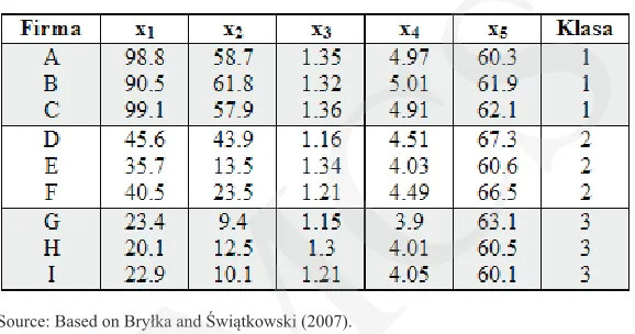
Example: The application of neural networks in risk estimation

The problem is to classify a company X into one of the three classes/levels of risk: • low risk (good inancial condition/standing),

• moderate risk (average inancial condition), • high risk (bad inancial condition),

(12)

16 IJSR

6

based on ive characteristics x1, x2, x3, x4, x5, which form the vector of characteristic xT

= [x1, x2, x3, x4, x5] =[74.5, 48.2, 1.27, 4.1, 61.1]

The companies that were classiied into three risk classes have been investigated; the results are presented in Table 2.

The following neural network was deined to solve the problem (Figure 6).

x

1

N

1

x

2

N

2

x

3

N

3

x

4

x

5

w01

w02

w03

The network output has the values/parameters y1 = f(xT W1), y2 = f(xT W2), y3 = f(xT W3).

The genetic algorithm shall determine the values of the weight vectors W.

Neuron 1

W1= [-1, 0.008, 0.009, 0.001, 0.002, 0.003]T

Neuron 2

W2= [-159.2, 0.04, -0.12, -16.89, -5.35, 3.14]T

Neuron 3

W3= [-.15, -0.03, 0.01, -0.2, -0.02, 0.02]T

Table 2.

Examples of historical/back data risk assessment

Figure 6.

The scheme of neural network