Article
Resource Demand Forecasting Model Based on
Dynamic Cloud Workload
Chunyan An 1, Jiantao Zhou 1,*
1 College of Computer Science, Inner Mongolia University, Hohhot, China; [email protected] * Correspondence: [email protected];
Abstract: The primary attraction of IaaS is providing elastic resources on demand. It becomes imperative that IaaS-users have an effective methodology for learning what resources they require, how many resources and for how long they need. However, the heterogeneity of resources, the diversity resource demands of different cloud applications and the variation of application-user behaviors pose IaaS-users big challenge. In this paper, we purpose a unified resource demand forecasting model suiting for different applications, various resources and diverse time-varying workload patterns. With the model, taking input from parameterized applications, resources and workload scenarios, the corresponding resources demands during any time interval can be deduced as output. The experiments configure concrete functions and parameters to help understanding the above model.
Keywords: cloud computing; workload model; workload-aware resource forecasting model
1. Introduction
At present, ever-increasing enterprises, SMBs (Small-and-Medium-sized Businesses) and organizations are running their applications on IaaS (Infrastructure as a Service) [1]. To take true advantages of IaaS, IaaS-users need to be able to rent the resources really on demand. For that, IaaS-users need to compare alternatives IaaS resources when building new systems, to assess capacity of selected resources when setting up systems, to adjust the use of cloud resources dynamically during running of the system.
However, with the development of cloud computing, IaaS-users face a bigger challenge. The challenges are mainly from the following reasons:
(1) The heterogeneity of IaaS resources
Different IaaS providers usually have different system design and system implementation. Besides, each IaaS provider provides a number of different optional IaaS resources. Moreover, different cloud environments are the different combinations of cloud resources across multiple hybrid clouds. To evaluate and compare different cloud environments is a big challenge.
(2) The diversity of applications
With the adoption of clouds in more and more areas, even including traditional areas, the type of cloud applications is more diverse [2]. Different applications, even if belong to the same area, the demand for cloud resources may have very big difference.
(3) The complexity of user behaviors
In reality, multiple applications are often deployed in one cloud environment. At the same time, end users are from around the world, they request the applications according to their own habits and requirements. This makes the user behaviors more complex. Thus the patterns of collective user behaviors, i.e. the workload patterns in this paper, have more possibilities.
Benchmarks[3] in cloud computing solve the first challenge partly. Benchmarks generate a select set of workloads that can be ported to different cloud environments and used as the basis for comparison and evaluation. However, most Benchmarks are either domain specific, like Rubis[4] for e-business, or programming-model specific, like MapReduce[5] etc. Even if the applications of IaaS-users belong to the similar domain or similar programming-model of the respective
benchmarks, the result from the benchmarks can be very different from the actual running result. Another shortcoming of benchmarks is the workload patterns defined in a benchmark are too limited to cover the possible workload scenarios.
Workload modeling is another option to address the above challenges. Workload modeling is to set up general statistical model, which can be used to generate synthetic workloads. In [6], workload models are classified into two types: descriptive models and generative models. Descriptive models mimic realistic workload traces mostly by fitting distributions. Generative models simulate user behaviors at the first place. This paper falls into basically generative models with an attempt of higher abstraction degree.
This workload modeling provides a general definition for cloud applications, which is suitable to specify most of cloud applications. Moreover, this paper offers a general statistical model, which can be used to generate diverse workload patterns. The generated workload here actually is a collection of end user requests to the applications. The statistical model specifies how the collective user requests change over time. Then, based on the workload modeling, the numbers of each basic service units in every certain period are computed out. Since the mean execution times of each basic service units running on each resource type can be measured, thereby the demands to a cloud environment in every certain period are to be estimated. In the previous work [7], a hierarchical workload modeling was proposed. In this work, the workload modeling is improved and based on the workload modeling a transformation methodology between the workload and resource demand is presented.
The remainder of this paper is organized as follows: Section 2 presents the existing related works. Section 3 specifies the workload modeling approach and resource demand estimation approach. Section 4 illustrates the process of generating workload based on workload model with an example. The last, Section 5 is a conclusion and discussion of the future work.
2. Related Works
This section may be divided by subheadings. It should provide a concise and precise description of the experimental results, their interpretation as well as the experimental conclusions that can be drawn. The challenges on cloud application workload modeling and workload-aware cloud infrastructure resource prediction have attracted many researchers. The related works will be specified in four aspects: workload population modeling/cloud application modeling, workload variation modeling, cloud infrastructure resource modeling and workload-aware resource prediction.
• Cloud application modeling
support multi-application-types workloads in reality. At present, we see the efforts in general cloud application model from cloud service brokers (e.g. Cloud Application Template from RightScale[16] and international standards organizations(e.g. SPEC OSG Cloud Working Group of SPEC. OSG[2]). Our cloud application model attempts to build a consistent definition which can cover most of cloud application types.
• Workload variation modeling
Representativeness, reality and generalization are the requirements of most workload modeling. Existed workload models for cloud applications cannot meet all the three requirements.
(1) Benchmarks:
Many researchers and organizations have been devoting themselves to developing representative workload models as benchmarks, for examples [3], [17, 21]. However, the workload patterns in benchmarks are usually very limited, cannot span the spectrum of possible workloads. Moreover, a benchmark aimed at a specific application, cannot reflect real usage of applications of cloud users, even if they are in similar domain.
(2) Workload modeling based on trace:
In order to build a more realistic workload model, many researchers fitted out the mathematical workload models using trace logs from some cloud providers [22, 25]. Though a fitting model is closer to the reality than a model based on mathematical assumption, it can reflect only some specific workload patterns of specific cloud providers during some specific time periods.
(3) Abstract mathematic workload modeling:
Abstract mathematic workload modeling tries to capture the main characteristics of workloads or some workload patterns. Through the parameterization of abstract workload model, diverse workload models or specific workload models conformed to some workload patterns can be produced. For example, [26] gave a methodology of building a burst workload model. The idea that generated a spike workload by superposition of normal workload and increasing workload inspired our work. [27] used periodicity and burstiness to specify and workloads in order to classify the workloads for elastic resource provision. [28] proposed a Hierarchical Bundling Model (HIBM) to model inter-arrival process. Our workload model falls into abstract mathematic workload modeling. We constructed a dynamic hierarchical workload model. On each layer two main variations are captured: number and mix. Then the superposition the variations of each layer produced the final workload model. Our model is so general that diverse workload patterns can be generated.
• Cloud infrastructure resource modeling
Cloud Infrastructure Resource consists of mainly CPU, memory, storage, disk I/O and network. Most Mainstream IaaS providers, like Amazon, RackSpace, provide different types of VMs (Virtual Machines). Each type of VM is configured with a set of resources. VM instances are the basic units of resource allocation. Therefore, many researchers modeled infrastructure resources as VMs [29, 31]. Some researchers defined an infrastructure resources as a set {R1,……Rm}, in which Rk (k=1..m) is a given level capacity (e.g. CPU, memory, storage, disk I/O and network)[32]. Some researchers [24] concerned about the detailed consumptions of individual hardware (e.g. CPU, memory, disk). Since the objectivity of this paper is to help a cloud user to manage their rented infrastructure resources, the resource model is based on VM.
• Workload-aware resource prediction
The research of workload-aware resource prediction includes two parts: (1) at some time point, the relationship of the amount of workload and the needed resources. (2) in a certain workload scenario (e.g. burst or diurnal pattern), the correspondence between workload fluctuation and the variation of resource requirements. For example, [14] used KCCA (Kernel Canonical Correlation Analysis) method to predict the execution time of MapReduce jobs. And [33] studied the optimized resources scaling options based on workload variation under the premise of ensuring SLA. The work in this paper has done the first part transforming the workload into the amount of basic execution units, which is the base of prediction of resource requirements.
Workload model includes two parts: a standard cloud application model and a workload variation model. Cloud application model includes a group of service unit specifications and the dependencies between the service units. A right stochastic matrix defines the dependencies between the service units. The stochastic matrix specifies the probabilities of users moving from service unit i to service unit j. This model is suitable for describing the cloud applications in which the service units are loosely-coupled or independent (e.g. web applications) or the service units are sequentially executed (e.g. MapReduce). And the model is not suitable for specifying the complex workflow application which includes control flow dependencies like Synchronize. Considering that loosely-coupled web applications and map-reduce applications covered most of cloud applications, we choose a stochastic matrix to specify the dependencies between service units rather than DAG (Directed Acyclic Graph) [7].The workload variation model abstracts main characteristics of workload variations. Here workload variation is abstracted a compound arrival process, which specify arrival process, popularity of service units, data-size or computation-scale distribution of each service unit. Workloads which are generated based on the workload model are a set of mixed requests to different service units. Then the requests to different service units are normalized into basic execution units. Last, the requests during any time interval are transformed into the numbers of needed resources. The models are detailed in the following four sub-sections.
3.1. Application Model
An Application is specified by A = ( S (A ), D(A ), C(A ) ), where S (A ) = { … } is a finite set of service unit types, D(A ) is a n × n matrix to specify the probability links between the service units, C(A ) is a constant to specify the input unit data size.
About S (A ) = { … }, ( = 1, … ) means a service unit type in the application A, n is the number of service units types in the application. Here is additional service unit, which means exit state.
And in D(A ),
p s , s
denotes the probability that service unit links next to .D(A ) =
p(s , s ) p(s , s ) …
p(s , s ) ⋱
… p s , s
p(s , s )⋮
p(s , s ) … p(s , s )
(1)
Where
1. p si, sj 0, i, j = 1,2, … n
2. ∑ p s , s = 1
3. p(s , s ) = 0, if i ≠ n
p(s , s ) = 1
We assume that user can stop the request with some probability after performing any service unit.
p(s , s )
is the probability, after performing service units
, that the user will stop the request.We choose Markov matrix to specify the processing dependencies between service units are based on the following belief:
(1) Most web-based Applications are loosely coupled. That means the service units in an application have no complex processing dependencies like join/split. The Markov matrix can specify all the possible processing orders and user preferences.
(2) Map-Reduce Applications usually include map->shuffle->reduce three service units, and the three units execute sequentially. So the Markov matrix specifying a map-reduce application will be like this:
i) A = ( S (A ),D(A ), C(A ))
ii) S(A ) = {map, shuffle, reduce, end}
iii) D(A ) =
0 1 0 0 0 01 0 0 0 0 0 0 1 0 1
3.2. Infrastructure Resource Model and Service Unit Execution Time Definition
Firstly, a VM (Virtual Machine) type VM is defined by a capacity consisting of a group of optional infrastructure hardware ((CPU, CPU number), (Memory, Memory Size), (Disk, Storage Size), (Network, Bandwidth)).
Secondly, on a VM(Virtual Machine) type VM , the basic execution times of service units of application Ai is defined as a T(VM , A ) = (t(VM , s ), … t(VM , s ),0), in which t(VM , s ) represents the mean execution time of service unit s with input unit data size C(A ) on a VM .
t(VM , s )=0 because s is the exit service unit, which executes null. The other t VM , s ( =
1,2, … − 1) satisfy with t VM , s > 0. The basic execution time of Application A on VM is defined as BasicTime(VM , A ) = min{t(VM , s ), (j = 1,2, … n − 1)}.
Thirdly, for each service unit s , there exists a scaling function f (x , VM ), x is the input data size, f (x , VM ) is the execution time of service unit s on VM with the input data size x .
f (x , VM ) describes the relationship between input data size and execution time on VM for service unit s.
Lastly, a basic service unit here means a service unit which has a basic input data size or a basic computational scale. A set of basic service units of application A is defined as n × 1 matrix
Basic VM , A = b VM , s , … b VM , s , 0 . b VM , s > 0, j ≠ n represents the basic input unit of service unit s on VM . And b VM , s = 0 because s is the exit service unit, whose input is null.
For normalization, each b VM , s ,j ≠ n should choose appropriate value to make
f b VM , s , VM = BasicTime VM , A . That means, the execution times of all basic service units
except s are equal to BasicTime VM , A .
3.3.Workload Variation Model
For simplifying the problem, the workload consists of one application type. In a time interval new requests consist of two parts: new arrival requests and transform requests. New arrival requests are the requests to the service units which are belong to the set of start service units of an application; Transform requests are determined by the dependencies between service units in an application.
Firstly, the workload variation during a short interval(t, t + τ], 0 < τ < BasicTime VM , A is computed. There are two properties of the interval( , + τ].
(1) In this interval, the new arrived requests for will not transform to next service unit. (2) In this interval, the currently existing service units arrived before t can only transform to next one step.
All requests during an interval (t , t ] are defined as follows: i. Inter-arrival process is defined as follows:
(1) Mean arriving rate
If start time is 0, until time t the mean of the number of arrived requests for A is N(A , t), then
N(A , t + τ ) − N(A , t)]/τ is called the mean arriving rate of requests for A during an
interval( , + τ]. The arriving rate at some time point t is
α(A , t ) = lim
→ N(A , t + τ ) − N(A , t)]/τ = d( N(A , t)) dt⁄ (3) So the mean arriving rate of requests for A during the interval is (t, t + τ]
a(A , t, t + τ) = α(A , t )dt τ (4) And the mean of the number of arrived requests for is during an interval (t, t + τ]
N(A , t, t + τ ) = α(A , t )dt (5) (2) Compound arriving process considering the popularity of different service units in
PR = PR (s⋯ )
PR (s ) and satisfied ∑ PR s = 1 (6)
Let S(Aistart) denote the set of all possible service units to which new arrived Ai requests refer. If s j ∉ S(Aistart), then PR s = 0; Obviously, s is exit service unit, so s ∉ S(A ), PR (s ) = 0.
Assume during an interval (t, t + τ], if the arriving rate at some time point t of requests for s is α A : s , t , and the mean of the number of arrived requests for s is N A : s , t, t + τ , then
N A : s , t, t + τ = α A : s , t dt (7) in which
α A : s , t = PR (s )α(A , t ) (j = 1,2 … n) (8) So
N A : s , t, t + τ = PR (s )α(A , t )dt (9) And
N(A , t, t + τ ) = ∑ N A : s , t, t + τ (10)
Define a 1 × n matrix N (A , t, t + τ) as the numbers of arrived requests for each s of Application A during an interval (t, t + τ],
N (A , t, t + τ) = N(A : s , t, t + τ ), ⋯ N(A : s , t, t + τ ) (11) (3) Compound arriving process considering bulk arrival.
If each arrived request for each s (j = 1,2 … n) of Application A could include multiple basic service unit s, then the arrival process is called bulk arrival process. Let random variable Z represent the number of basic service unit s in each arrived request for s , its probability mass function is P z = P Z = z , z 0 and the mean of Z is E Z ]. Let us define Z , , Z , , …
as the iid sequential numbers of basic service units, the number of basic service unit s during an interval (t, t + τ], N A : s , t, t + τ is given by
N A : s , t, t + τ = ∑ : , , Z , (12)
Define a 1 × n matrix N (A , t, t + τ ) as the arrived numbers of each service unit of Application A during an interval (t, t + τ]
N (A , t, t + τ)= N (A : s , t, t + τ ), ⋯ N (A : s , t, t + τ ) (13) ii. Transform requests during the interval (t, t + τ] are defined as follows:
Assume the numbers of currently existing service units of Application A at time t is defined as a 1 × n matrix Ɲ (A , t)
Ɲ (A , t) = Ɲ (A : s , t ), ⋯ Ɲ (A : s , t ), Ɲ (A : s , t ) (14)
Then after one step transform, the numbers of transformed service units during the interval
(t, t + τ] is defined as Ɲ(A , t, t + τ)
Ɲ(A , t, t + τ) = Ɲ (A , t) ∗ D(A ) (15)
= Ɲ (A : s , t ) ⋯ Ɲ (A : s , t )
p(s , s ) p(s , s ) …
p(s , s ) ⋱
… p s , s
p(s , s )⋮
p(s , s ) … p(s , s )
From the equitation 15, the each Ɲ A : s , t, t + τ can be computed out,
Ɲ A : s , t, t + τ = ∑ Ɲ (A : s , t ) ∗ p s , s (16) iii. All requests during the interval(t, t + τ]are defined as follows:
Ɲ (A , t + τ) is the sum of the new arrived service units during (t, t + τ] and the one-step transformed service units during (t, t + τ].
Ɲ (A , t + τ) = N (A , t, t + τ) + Ɲ(A , t, t + τ) (17)
= N (A , t, t + τ) + Ɲ (A , t) ∗ D(A ) (18) iv. All requests during an interval (t , t ] are defined as follows:
(1) = min {k ∈ |k }, k is the numbers of transforms during(t , t ], its value is the smallest integer not less than . (19)
(2)Based on Eq.(18), the numbers of each service units of Application Ai at time t + jτ can be deduced by
Ɲ (A , t + jτ) = N (A , t + (j − 1)τ, t + jτ) + Ɲ (A , t + (j − 1)τ) ∗ D(A ) (20)
(3)Finally, after k loop iterations, the numbers of each service units of Application A at time
t are computed out:
Ɲ (A , t ) = N (A , t + (k − 1)τ, t ) + ∑ N (A , t + (j − 1)τ, t + jτ) ∗ D(A ) ] + Ɲ (A , t ) ∗
D(A ) (21)
3.4. Resource Forecasting
To forecast the demands of during an interval( , ] , firstly, define a workload
( , , ) is a 1 × matrix, is as same as Eq.(19).
W (A , t , t ) = (Ɲ ( , ), Ɲ ( , + τ),… , Ɲ ( , t )) (22)
Then, define a 1 × matrix ( , ( , , )) as the numbers of needed for Application during an interval ( , ].
( , ( , , )) = (Ɲ ( , ), Ɲ ( , + ),… , Ɲ ( , ))/ ( , ) (23)
Where (VM , A) means the maximal number of parallel basic service units on one
VM with an acceptable performance or satisfied with some SLA (Service Level Agreement). Table 1 lists the important annotations in the model.
Table 1. The Annotations in the Model
Annotations Type Description
A = ( S (A ), D(A ), C(A ) )
tuple application definition
S (A ) set a finite set of service unit types
D(A ) n × n matrix specify the probability links between the
service units
C(A ) int specify the input unit data size
VM tuple VM(Virtual Machine) type definition
T(VM , A ) 1×(n-1) matrix the basic execution times of service units of
application A is defined as a T(VM , A ) =
(t(VM , s ), … t(VM , s ),0),, in which t(VM , s ) represents the mean execution time of service unit s with input unit data size C(A ) on a VM
BasicTime(VM , A ) float The basic execution time of Application A
on VM is defined as BasicTime(VM , A ) =
min{t(VM , s ), (j = 1,2, … n − 1)}.
f (x , VM ) function f (x , VM )) describes the relationship
between input data size and execution time on
VM for service unit s.
Basic VM , A 1 × n matrix A set of basic service units of application
A is defined as Basic VM , A =
b VM , s , … b VM , s , 0 . b VM , s >
unit s on VM
α(A , t ) float describes the arriving rate at some time point
t
a(A , t, t + τ) float the mean arriving rate of requests for
A during an interval (t, t + τ]
N(A , t) int If start time is 0, until time t the mean
number of arrived requests for A
N A : s , t, t + τ int The mean number of arrived requests fors
during an interval (t, t + τ]
N (A , t, t + τ) 1×n matrix the numbers of arrived requests for each s
of Application A during an interval (t, t + τ]
Z int represent the number of basic service units
in each arrived request for s
N A : s , t, t + τ int the number of basic service unit s during an
interval (t, t + τ]
4. Experiments
In this section, a simple example of workload generation process is given to show how to generate a workload based on a workload model.
i. Workload model definition (1) application definition A = ( S (A ), D(A ), C(A ) ) S (A ) = {S1, S2, S3, end}
D(A ) =
0.28 0.21
0.40 0.18 0.28 0.23 0.27 0.15 0.28 0.27
0 0 0.29 0.16 0 1
(2) workload variation definition time interval τ = 1
=
0.16 0.48 0.36 0
Arriving process is possion process with parameter λ=3, abbreviated to PP(λ=3). ii. Workload generation process
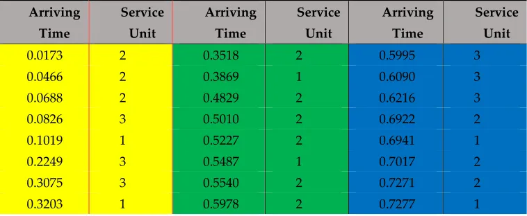
(1) Generate 40 service unit requests: arriving times are generated conformed to PP(λ=3), arriving service units are generated randomly according to . The detail is shown in Table2.
Table 2. The Annotations in the model.
Arriving Time
Service Unit
Arriving Time
Service Unit
Arriving Time
Service Unit
0.0173 2 0.3518 2 0.5995 3
0.0466 2 0.3869 1 0.6090 3
0.0688 2 0.4829 2 0.6216 3
0.0826 3 0.5010 2 0.6922 2
0.1019 1 0.5227 2 0.6941 1
0.2249 3 0.5487 1 0.7017 2
0.3075 3 0.5540 2 0.7271 2
Arriving Time
Service Unit
Arriving Time
Service Unit
0.7518 2 1.1117 2
0.8386 3 1.1188 3
0.8727 3 1.2830 2
0.8903 2 1.3949 2
0.9359 1 1.4153 1
0.9987 2 1.6881 2
1.0007 3 2.2034 2
1.0435 2 2.2652 1
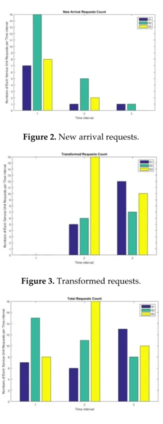
(2) As time interval τ = 1, count up the numbers of each service units arrived during each time interval. The detail is shown in Table 3.
Table 3. New arrival service unit requests per time interval.
Time Interval S1 S2 S3
1 7 15 8
2 1 5 2
3 1 1 0
(3) Count up the numbers of randomly transformed service units during each time interval. The detail is shown in Table 4.
Table 4. Transformed service unit requests per time interval.
First time interval S1 S2 S3 S4
From S1 to 0 2 4 1
From S2 to 4 1 9 1
From S3 to 1 3 3 1
Second time interval S1 S2 S3 S4
From S1 to 3 1 1 1
From S2 to 3 3 3 2
From S3 to 6 3 6 3
(4) Count up the total numbers of service units during each time interval.
Table 5. Total service unit requests per time interval.
Time Interval S1 S2 S3
1 7 15 8
2 6 11 18
3 13 8 10
Figure 1. Randomly generated requests arriving at passion process with λ=3.
Figure 2. New arrival requests.
Figure 3. Transformed requests.
Figure 4. Total requests.
5. Conclusions
In this paper, we proposed a projection methodology from a hierarchical workload model to the numbers of each basic service units in any time periods. When the execution-time and the scaling functions of each service unit on a VM are known, the needed infrastructure resources can be deduced by the numbers of each service units. The resource prediction model is general and flexible because the workload model has the advantages:
The workload model provides a generalization of both applications and workload variations. Different types of cloud applications are supported, for example, web applications, MapReduce applications. Since two main characteristics of workload variations are captured: the numbers and the mix, diverse workloads can be specified by parameterizing the workload model.
(2) Flexibility:
Application definitions are departed from workload variations. That means, a cloud user can pick up any possible workload patterns to test any their applications. Moreover, the workload model enables cloud users to modify the values of parameters in order to generate a workload fitting a certain situation. Furthermore, the multiple workloads generated by the workload model can be superposed. For example, a diurnal pattern workload can superpose a burst pattern workload.
In future, we put emphasis on refining the model of the relationship between the numbers of requests and the needed infrastructure resources. For that, we will design a set of experiments to measure different applications on different VMs.
Acknowledgement: This work is supported by National Natural Science Foundation of China [No.61662054 and No.61262082], and Inner Mongolia Technological Innovation Team Project “Cloud Computing and Software Engineering”. Thanks the students Jiajia Xu, Ruiqing Yan and Jing Yang for the help with the experiments.
References
1. RightScale. Cloud Computing Trends: 2016 State of the Cloud Survey from RightScale, 2016.
2. Milenkoski, a, Iosup, a, Kounev, S., Sachs, K., Ding, J., & Rosenberg, F.; Cloud Usage Patterns : A Formalism for Description of Cloud Usage Scenarios. Tech Report SPEC-RG-2013-001 v1.0.1, SPEC Research Group, 2013, 12–13.
3. Alexandru Iosup, Radu Prodan; IaaS Cloud Benchmarking : Approaches, Challenges, and Experience. MTAGS, 2012.
4. RUBiS. 2013.
5. Huang, S., Huang, J., Dai, J., Xie, T., & Huang; The HiBench benchmark suite: Characterization of the MapReduce-based data analysis. 2010 IEEE 26th International Conference on Data Engineering Workshops, ICDEW, 2010, 41–51. https://doi.org/10.1109/ICDEW.2010.5452747.
6. Feitelson, D. G.; Workload modeling for computer systems performance evaluation, 2010.
7. An, C., Zhou, J., Liu, S., & Geihs, K.; A multi-tenant hierarchical modeling for cloud computing workload. Intelligent Automation & Soft Computing, (May), 1–8. https://doi.org/10.1080/10798587.2016.1152774. 8. Bahga, A.; Synthetic Workload Generation for Cloud Computing Applications. Journal of Software
Engineering and Applications, 2011, 04(07), 396–410. https://doi.org/10.4236/jsea.2011.47046.
9. Beitch, A., Liu, B., & Yung, T.; Rain:A workload generation toolkit for cloud computing applicationsand Computer,2010.
10. Mao, M., & Humphrey, M.; Auto-scaling to minimize cost and meet application deadlines in cloud workflows. 2011 International Conference for High Performance Computing, Networking, Storage and Analysis (SC), 2011, 1–12. https://doi.org/10.1145/2063384.2063449.
11. Mao, M., & Humphrey, M; Scaling and scheduling to maximize application performance within budget constraints in cloud workflows. Proceedings - IEEE 27th International Parallel and Distributed Processing Symposium, IPDPS, 2013, 67–78, https://doi.org/10.1109/IPDPS.2013.61.
12. Iosup, A., Sonmez, O., Anoep, S., & Epema, D.; The performance of bags-of-tasks in large-scale distributed systems. In Proceedings of the 17th international symposium on High performance distributed computing - HPDC, 2008, (p. 97). New York, USA: ACM Press. https://doi.org/10.1145/1383422.1383435.
13. Oprescu, A., & Kielmann, T.; Bag-of-tasks scheduling under budget constraints. Cloud Computing Technology and Science. IEEE Computer Society, 2010:351-359.
14. Ganapathi, A., Chen, Y., Fox, A., Katz, R., & Patterson, D.; Statistics-driven workload modeling for the cloud. Proceedings - International Conference on Data Engineering, 2010, 87–92. https://doi.org/10.1109/ICDEW.2010.5452742.
16. RightScale. IT AS A CLOUD SERVICES BROKER : Provide Self-Service Access to Cloud, 2014.
17. Gillam, L., Li, B., O¿Loughlin, J., & Tomar, A. P.; Fair Benchmarking for Cloud Computing systems.
Journal of Cloud Computing: Advances, Systems and Applications, 2013, 2(1).
https://doi.org/10.1186/2192-113X-2-6.
18. Huang, S., Huang, J., Liu, Y., Yi, L., & Dai, J.; HiBench: A Representative and Comprehensive Hadoop Benchmark Suite. ICDE Workshops, 2010. 192.198.165.138. Retrieved from http://192.198.165.138/sites/default/files/blog/329037/hibench-wbdb2012-updated.pdf.
19. Moschetta, J., & Casale, G; OFBench.: An enterprise application benchmark for cloud resource management studies. Proceedings - 14th International Symposium on Symbolic and Numeric Algorithms for Scientific Computing, SYNASC, 2012, 393–399. https://doi.org/10.1109/SYNASC.2012.39.
20. TPC-W Web Commerce Benchmark, 2006.
21. Turner, A., Fox, A., Payne, J., & Kim, H. S.; C-MART: Benchmarking the cloud. IEEE Transactions on Parallel and Distributed Systems, 2013, 24(6), 1256–1266. https://doi.org/10.1109/TPDS.2012.335.
22. Chen, Y., Alspaugh, S., & Katz, R.; Interactive analytical processing in big data systems: a cross-industry study of MapReduce workloads. Proceedings of the VLDB Endowment, 2012, 5(12), 1802– 1813.https://doi.org/10.14778/2367502.2367519.
23. Gong, Z., & Gu, X.; PAC: Pattern-driven application consolidation for efficient cloud computing. Proceedings - 18th Annual IEEE/ACM International Symposium on Modeling, Analysis and Simulation of Computer and Telecommunication Systems, 2010, 24–33. https://doi.org/10.1109/MASCOTS.2010.12.
24. Moreno, I. S., Garraghan, P., Townend, P., & Xu, J.; Analysis, Modeling and Simulation of Workload Patterns in a Large-Scale Utility Cloud. IEEE Transactions on Cloud Computing, 2014, 2(2), 208–221. https://doi.org/10.1109/TCC.2014.2314661.
25. Li, H.; Realistic workload modeling and its performance impacts in large-scale escience grids. IEEE Transactions on Parallel and Distributed Systems, 2009, 21(4), 480–493. https://doi.org/10.1109/TPDS.2009.99. 26. Bodik, P., Fox, A., Franklin, M. J., Jordan, M. I., & Patterson, D. a.; Characterizing, modeling, and
generating workload spikes for stateful services. Proceedings of the 1st ACM Symposium on Cloud Computing - SoCC, 2010, d, 241. https://doi.org/10.1145/1807128.1807166.
27. Ali-eldin, A., Tordsson, J., Elmroth, E., & Kihl, M.; Workload Classification for Efficient Auto-Scaling of Cloud Resources, Computer Systems, 2013, 1–36.
28. Juan, D. C., Li, L., Peng, H. K., Marculescu, D., & Faloutsos.; Beyond poisson: Modeling inter-arrival time of requests in a datacenter. Lecture Notes in Computer Science (Including Subseries Lecture Notes in Artificial Intelligence and Lecture Notes in Bioinformatics), 2014, 8444 LNAI (PART 2), 198–209. https://doi.org/10.1007/978-3-319-06605-9_17.
29. Vakilinia, S., Ali, M. M., & Qiu, D.; Modeling of the resource allocation in cloud computing centers. Computer Networks, 2015, 91, 453–470.,https://doi.org/10.1016/j.comnet.2015.08.030.
30. Calheiros, R. N., Ranjan, R., De Rose, C. A. F., & Buyya, R.; CloudSim: A Novel Framework for Modeling and Simulation of Cloud Computing Infrastructures and Services. 2009, arXiv Preprint arXiv: 0903.2525, 9. Retrieved from http://arxiv.org/abs/0903.2525.
31. Wu, L: SLA-based Resource Provisioning for Management of Cloud-based Software-as-a-Service Applications. PhD Thesis, University of Melbourne, 2014, March.
32. Tsai, J.-T., Fang, J.-C., & Chou, J.-H.; Optimized task scheduling and resource allocation on cloud computing environment using improved differential evolution algorithm. Computers & Operations Research, 2013, 40(12), 3045–3055. https://doi.org/10.1016/j.cor.2013.06.012.